An empirical study on coordinated development of energy consumption structure and green total factor productivity under spatial interaction

Abstract

Existing studies have found a non-linear relationship between the energy consumption structure (ECS) and the green total factor productivity (GTFP), but their influencing factors are not yet clear. This study examines the spatial impact of existing green development measures on coordinating the ECS and the GTFP using the coupling and spatial econometric models. The research findings are as follows: (1) The coordination between the ECS and the GTFP has increased over time, and the coordination is significantly higher in economically developed cities. (2) The spatial analysis results show a significant spatial auto-correlation between the ECS and the GTFP coordination. Green development approaches such as environmental regulations, technological innovations, and industrial structure significantly contribute to the degree of coordination. Decomposition of the spatial effects shows that technological innovations significantly affect local and neighbouring cities. These conclusions hold after endogeneity and robustness tests. The results suggest that local governments in city clusters should promote environmental regulations, industrial structure, and technological innovations to promote the coordinated development of the ECS and the GTFP of urban agglomerations.

Keywords:

• Energy consumption structure
• green total factor productivity
• spatial lag model
• urban agglomeration

JEL CLASSIFICATIONS:

• C33
• Q43
• R11

1. Introduction

The world has entered an era of global climate change, which has become one of the most severe environmental threats to humans (Wang et al., 2021). As the world's most populous country and the largest carbon emitter (UNEP Copenhagen Climate Centre [UNEP-CCC], 2021), China must perform a critical role in resolving the global climate change crisis. In 2020, the Chinese government proposed to achieve carbon peaking by 2030 and carbon neutrality by 2060 by establishing a series of staged plans with a series of phased plans (Central Committee of the CPC & the State Council, 2021). However, a sudden and concentrated outbreak by some local governments cut-off power supply during the peak production season. The Chinese official media criticised a few local governments for their reckless 'one-size-fits-all' demands before the assessment to meet the central government's requirements. This phenomenon reveals not only the 'short-sighted' behaviour of local governments but also the confusion about meeting the Central government's goals of 'optimising energy consumption structure' and 'maintaining a green and medium-high economic growth rate' at the same time (Feng et al., 2009; Zhang et al., 2013), especially in the context of sustainable development policymaking in all developing countries.

Many studies have suggested energy consumption structure (ECS) and green total factor productivity (GTFP) improvements in different fields (Sharma et al., 2021; Tseng et al., 2021; Xie et al., 2021). Additionally, studies have identified that the relationship between the ECS and the GTFP is close but non-linear, and ECS optimisation can improve the GTFP only within a moderate range (Xie, Zhang, & Wang et al., 2021). Therefore, are there influences that can achieve a coordinated and simultaneous increase in the ECS and GTFP? Is there a spatial correlation between the coordination of the ECS and the GTFP in urban agglomerations? In this spatially interactive perspective, what are the spatial and temporal characteristics of the factors influencing the ECS and GTFP? These questions still need to be addressed. Based on theoretical analysis and empirical tests, this study explains the mechanisms and effects of improving the ECS and GTFP coordination (EGC), denoted as $\mathit{EGC},$ which is of practical significance for local communities to achieve dual enhancement of ECS and GTFP.

The main academic contributions and innovations of this study are: (1) to explore the mechanism of achieving the $\mathit{EGC}$ in general; (2) to explore the spatial and temporal characteristics of the $\mathit{EGC};$ and (3) through empirical research, analyse the factors that influence the $\mathit{EGC},$ and provide policy implications.

The remainder of this article is organised as follows: Section 2 is the literature review; Section 3 is the method and data; Section 4 is empirical results; finally, Section 5 is the conclusion and policy implications.

2. Literature review

ECS improvement refers to a reduction in the use of fossil fuels such as coal, oil, and natural gas. For a long time now, along with the growth of total economic volume, local energy demand has also continued to increase (Bakirtas & Akpolat, 2018; Huang et al., 2021; Zheng & Walsh, 2019). Industrial enterprises that rely on fossil energy under the pressure of local government environmental regulations must face the choice of green transformation or closure (Wang et al., 2020; Yang et al., 2021). However, green transformation does not occur overnight but only after a threshold of local environmental regulations has been reached (Shen et al., 2020).

Industrial firms must improve their competitiveness through technological innovations to meet environmental regulation needs. However, according to Porter's hypothesis (Porter & Van der Linde, 1995) and subsequent research, the impact of environmental regulations on green technological innovations is non-linear (Du et al., 2021; Töbelmann & Wendler, 2020; Zhou et al., 2021). This implies that the ECS can only be improved if environmental regulations and technological innovations reach a certain level concurrently. In addition to industrial enterprises, the development of the service industry also has a significant positive effect on the improvement of the ECS (Luan, Zou, Chen, & Huang et al., 2021). With the development of the digital economy and the Internet, and the impact of the sharing economy on energy efficiency improvements (Dabbous & Tarhini, 2021), the dependence of certain industries on fossil energy will decrease (Ren et al., 2021), thus improving the ECS.

The GTFP is also influenced by environmental regulations (Shen et al., 2019), technological innovations (Wang et al., 2021), and the industrial structure, additionally, the GTFP is affected by improvements in the ECS. However, existing studies found that if the improvement in the ECS is insignificant, it will have an insignificant effect on the GTFP, and a highly significant improvement is detrimental to the green transition of industrial enterprises as well as to the GTFP. So, this relationship proves to be non-linear (Pegkas, 2020), suggesting that the relationship between the ECS and GTFP is not always coherent.

The existing research gap shows that although studies have discussed the relationship between the ECS and GTFP and their external influences separately, it is relevant to discuss how the $\mathit{EGC}$ can be enhanced given their inherently non-linear relationship. Zafar et al. (2020) empirical analysis of the OECD countries suggests that renewable energy sources contribute significantly to economic growth. This view is corroborated by Saint Akadiri et al. (2019) empirical study of EU-28 countries. However, Maji et al. (2019) used empirical data from West Africa and found that an optimised ECS impedes productivity growth. From the perspective of sample selection, the differences in research findings appear to be related to the country's level of development. Chen et al. (2020) empirically analysed more than 80 countries and found a non-linear relationship between the ECS and economic development, especially in developing countries. Additionally, existing studies show that an increase in urban density due to the current pace of urban construction in certain developing countries has led to an auto-correlation effect between the ECS and GTFP in space (Xie et al., 2021). Then, is there a spatial auto-correlation effect on the $\mathit{EGC}$? What are the spatial characteristics of the factors that influence the degree of coordination? This study addresses these questions, and that constitutes its innovative points and main academic contributions.

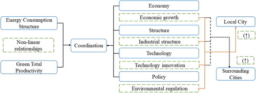
The existing literature reveals that the $\mathit{EGC}$ is analysed in four dimensions: economy, structure, technology, and policy (Zeng et al., 2021). The impact of economic growth on the ECS and GTFP is significant, and the gross domestic product (GDP) is an important part of the GTFP calculation. Industrial structure impacts both the ECS and GTFP. Technological innovation is critical for increasing the GTFP; it can also increase the use of clean and efficient energy in society and lead to continuous improvements in the efficient use of primary energy. Environmental regulations are critical for addressing negative externalities and market failures in environmental issues and for enhancing ecological and environmental protection. In conjunction with the above, this study presents the first hypothesis:

H1: Economic development, industrial structure, technological innovations, and environmental regulations have significant impacts on the $\mathit{EGC}.$

This study analyses from a spatial interaction perspective whether there are other features of the economic impact on the ECS and GTFP. First, economic growth, industrial structure, and technological innovations usually have a positive spatial spill-over effect on the central city (Murad et al., 2019) and neighbouring cities (Wang et al., 2021) and drive the overall local economic structure optimisation in neighbouring regions improving their ECS and GTFP. Second, existing studies have found that the spill over effects of environmental regulations on surrounding areas are both positive and negative, depending on the intensity, duration, and implementation of the regulations; therefore, this study presents the second hypothesis:

H2: The $\mathit{EGC}$ has significant spatial spill-over effects, with economic development, industrial structure, and technological innovations having a significant impact on local and neighbouring EGC, and environmental regulations have a significant impact only on the local EGC. An analytical framework for the $\mathit{EGC}$ was constructed (see Figure 1) according to the research hypothesis.

Figure 1. Theoretical analytical framework for the $\mathit{EGC}.$

Source: The author

3. Data and method

3.1. Overview of the study area

The sample chosen meets the following criteria: (a) This study analyses spatial data, and having smaller geographic units can avoid variable surface element problems. Thus, the geographic scale of the sample selected is the prefecture-level city. (b) According to the study's assumptions, the ECS and GTFP will not only affect local cities but will also be influenced by the effects produced by neighbouring cities. Therefore, urban agglomerations can more effectively verify the study's hypotheses. (c) China's current regional development strategy emphasises multi-distributed urban agglomerations, with the Yangtze River Delta urban agglomeration being among the country's few world-class examples with the highest population, economic output, urbanisation, and modernisation. As it is a critical pilot area for China's future regional economic development strategy, it is a typical sample to research. Moreover, the Yangtze River Delta urban agglomeration has implemented many innovative government policies and management methods. Hence, its experiences and lessons are instructive for other developing urban agglomerations, making the study’s conclusions universal. A schematic of the spatial distribution of the Yangtze River Delta urban agglomeration is shown in Figure 2.

Figure 2. Schematic of the spatial distribution of the Yangtze River Delta urban agglomeration.

Source: The author

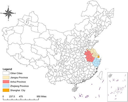
This study uses 41 cities above the prefecture-level in the Yangtze River Delta urban agglomeration in China from 2009 to 2019 as the study sample.

3.2. Measurement of ECS and GTFP coordination

Coupling is a physical concept mostly used in ecology and urbanisation studies (Xing et al., 2019). This study uses the coupling degree to reflect the $\mathit{EGC}$ through mutual interaction to express the phenomenon of mutual influence. It is necessary to reflect not only the interaction but also the coordination between them to avoid a pseudo-coordination situation where the coupling degree is high because of the similarity of the two scores (Tomal, 2021); therefore, the coupling coordination degree is used to reflect the coordinated development level of the two. (1) $$\begin{array}{c}D=\sqrt{C\mathrm{*}T}\\ T=\alpha U_1+\beta U_2\\ C=\frac{2\sqrt{{ES}_{it}\mathrm{*}{\mathit{GTFP}}_{it}}}{{ES}_{it}+{\mathit{GTFP}}_{it}}\end{array}$$(1) where$\mathrm{ }D\mathrm{ }$is the coupling coordination degree, the value range is [0,1], and the more significant value indicates the higher coupling degree. $T$ is the combined coordination value of the ECS and GTFP. $U_1$ and$\mathrm{ }{U}_2\mathrm{ }$represent the ECS and GTFP, respectively, which are the scores of these two subsystems. $\alpha \mathrm{ }$and$\mathrm{ }\beta$ are the relative weights, which are calculated using the entropy value method. $C$ is the coupling degree. Based on the $D$ value, this study classifies the $\mathit{EGC}$ into eight levels: severely dysfunctional ($D<0.2$); mildly dysfunctional ($0.2\le D<0.4$); on the verge of dissonance ($0.4\le D<0.5$); barely coordinated ($0.5\le D<0.6$); primary coordination ($0.6\le D<0.7$); moderate coordination ($0.7\le D<0.8$); good coordination ($0.8\le D<0.9$); and extreme coordination ($0.9\le D<1$). The level of coordination between the ECS and GTFP is uniformly recorded as$\mathrm{ }{\mathit{EGI}}_{it}.$

3.3. Spatial measurement model

Spatial econometrics is a reliable method for studying the spatial relevance of economic data across spatial units (Xu & Lee, 2019). (${\omega }_{ij}$) is the spatial weight matrix between the $i$-th city and the $j$-th city. The spatial weight matrix (${\omega }_{ij}$) of the model is determined by constructing the inverse distance spatial adjacency matrix based on the geographic coordinates of the 41 cities in the Yangtze River Delta urban agglomeration; see Equations (2)(2) $$\begin{array}{c}{\mathit{\omega }}_{\mathit{ij}}=\{\begin{array}{c}0 \left(i=k\right)\\ \frac{1}{d_{i,j}} \left(i\ne k\right)\end{array}\mathrm{ }\end{array}$$(2) and (3)(3) $$\begin{array}{c}{W}_{ij}=\left[\begin{array}{cc}\begin{array}{cc}0& {\omega }_{12}\\ {\omega }_{21}& 0\end{array}& \begin{array}{cc}\cdots & {\omega }_{1j}\\ \cdots & {\omega }_{2j}\end{array}\\ \begin{array}{cc}⋮& ⋮\\ {\omega }_{i1}& {\omega }_{21}\end{array}& \begin{array}{cc}\ddots & ⋮\\ \cdots & 0\end{array}\end{array}\right] \end{array}$$(3) . It is assumed that the spatial weight matrix does not change with time$\mathrm{ }t.$ (2) $$\begin{array}{c}{\mathit{\omega }}_{\mathit{ij}}=\{\begin{array}{c}0 \left(i=k\right)\\ \frac{1}{d_{i,j}} \left(i\ne k\right)\end{array}\mathrm{ }\end{array}$$(2) (3) $$\begin{array}{c}{W}_{ij}=\left[\begin{array}{cc}\begin{array}{cc}0& {\omega }_{12}\\ {\omega }_{21}& 0\end{array}& \begin{array}{cc}\cdots & {\omega }_{1j}\\ \cdots & {\omega }_{2j}\end{array}\\ \begin{array}{cc}⋮& ⋮\\ {\omega }_{i1}& {\omega }_{21}\end{array}& \begin{array}{cc}\ddots & ⋮\\ \cdots & 0\end{array}\end{array}\right] \end{array}$$(3)

3.4. Selection and calculation of variables

3.4.1. Data sources

All data were obtained from the Qianzhan (https://d.qianzhan.com/) and CEE (https://ceidata.cei.cn/) databases. The data in this study have been complemented by linear interpolation, and the indicators involving monetary measures are deflated by the consumer price index to eliminate the effect of inflation.

3.4.2. Calculation of ECS

The ECS is typically calculated in two ways. The first method reflects the ECS in the region by calculating the ratio of raw coal consumption to total regional energy consumption. The second method employs information entropy to characterise the orderliness and complexity of the ECS. To count the consumption of primary energy sources, such as coal, oil, and natural gas, the ratio of their information entropy and maximum entropy is computed, which is used to reflect the balance of primary energy consumption and, thus, the ECS. The current calibration of coal, oil, and natural gas consumption and supply in China's urban statistical yearbooks is inconsistent, so the second calculation method cannot be used. Therefore, this study used the proportion of regional raw coal consumption to the total regional energy consumption to represent the ECS.

3.4.3. Calculation of GTFP

The GTFP measures a city's level of green development and economic development efficiency when resource inputs and environmental costs are considered. This study uses the slacks-based measure in the data development analysis model (SBM-DEA) (Tone, 2001) to estimate urban GTFP. The Global Malmquist–Luenberger (GML) index is applied based on the SBM to measure the dynamics of the GTFP. The Solow residual method, the stochastic frontier analysis (SFA), the data envelopment analysis (DEA) and the SBM methods are the most frequently used calculation methods. The SFA method has the disadvantage of difficulty accounting for multiple outputs and the possibility of unexpected outputs. Additionally, the DEA method cannot solve for non-expected outputs (Streimikis & Saraji, 2021). Therefore, this study uses a non-radial, non-angle SBM-DEA model to quantify the GTFP, denoted as $GT\mathrm{F}P.$ The SBM-DEA model under consideration of non-desired outputs is shown in Equation (4)(4) $$\begin{array}{c}m\mathit{inGE}=\mathit{min}\frac{1-\left(\frac{1}{N}\sum _{n=1}^N\frac{s_n^x}{x^{t,k^{\mathrm{\text{'}}}}}\right)}{1+\left[\frac{1}{M+I}\left(\sum _{m=1}^M\frac{s_m^y}{y^{t,k^{\mathrm{\text{'}}}}}+\sum _{i=1}^I\frac{s_i^b}{b^{t,k^{\mathrm{\text{'}}}}}\right)\right]}\end{array}$$(4) . (4) $$\begin{array}{c}m\mathit{inGE}=\mathit{min}\frac{1-\left(\frac{1}{N}\sum _{n=1}^N\frac{s_n^x}{x^{t,k^{\mathrm{\text{'}}}}}\right)}{1+\left[\frac{1}{M+I}\left(\sum _{m=1}^M\frac{s_m^y}{y^{t,k^{\mathrm{\text{'}}}}}+\sum _{i=1}^I\frac{s_i^b}{b^{t,k^{\mathrm{\text{'}}}}}\right)\right]}\end{array}$$(4)

The constraints are： $$\sum _{k=1}^K{\lambda }_k^t{x}_{kn}^t+s_n^x=x_{k^{\mathrm{\text{'}}}n}^t,\mathrm{ }\forall n$$ $$\sum _{k=1}^K{\lambda }_k^t{y}_{km}^t-s_m^y=y_{k^{\mathrm{\text{'}}}m}^t,\mathrm{ }\forall m$$ $$\sum _{k=1}^K{\lambda }_k^t{b}_{ki}^t+s_i^b=b_{k^{\mathrm{\text{'}}}i}^t,\mathrm{ }\forall i$$

${\mathrm{ }{\lambda }_k^t\ge 0,\mathrm{ }\forall k,s}_n^x\ge 0,\mathrm{ }\forall n;\mathrm{ }{s}_m^y\ge 0,\mathrm{ }\forall m;\mathrm{ }{s}_i^b\ge 0,\mathrm{ }\forall \mathit{iGTFP},$ denoted as $\rho ,$ and 0 < ρ ≤ 1. The input vector, the desired output vector, and the non-desired output vector of city k′ at moment t, are denoted as $x^{t,k^{\mathrm{\text{'}}}},y^{t,k^{\mathrm{\text{'}}}},b^{t,k^{\mathrm{\text{'}}}},$ respectively. Slack vectors representing input-output, desired output, and non-desired output are denoted as $S^x,S^y,S^b,$ respectively. When $\rho =1,$ it indicates that the $\mathrm{G}\mathit{TFP}$ is efficient; when $\rho <1,$ it indicates that the $\mathit{GTFP}$ is inefficient.

The indicators selected to calculate the GTFP include three categories of indicators: input, desired output, and non-desired output. The input indicators include capital, labour, and resources. Fixed asset investment represents capital input. The number of employed persons per unit in urban areas represents the labour input. The built-up area represents land resource input; total water supply represents water resource input; total social electricity consumption represents energy input. The desired output indicator is the GDP, and the non-desired output indicators have negative impacts on the urban environment, including industrial wastewater emissions, industrial sulphur dioxide emissions, and industrial smoke and dust emissions.

As $\rho$ can only represent static efficiency values, this study chose to measure dynamic changes in efficiency values by including the GML index of non-desired output (Wang et al., 2020). The GML index is used with non-desired outputs to measure changes in the GTFP because traditional indices are used to measure changes in the GTFP, such as the Malmquist index, without non-desired outputs. The Luengerber productivity index and the Malmquist–Luenberger index are non-transmissible and have the disadvantage of having no feasible solutions (Oh, 2010), whereas the GML can address both drawbacks. Therefore, the GML index was chosen to represent dynamic changes in the GTFP.

First, the global SBM directional distance function under consideration of resource environment constraints is calculated as (5) $$\begin{array}{c}{\overrightarrow{S}}_v^G\left(x^{t,k^{\mathrm{\text{'}}}},y^{t,k^{\mathrm{\text{'}}}},b^{t,k^{\mathrm{\text{'}}}},g^x,g^y,g^b\right)=\begin{array}{c}max\\ S^x,S^y,S^b\end{array}\frac{\frac{1}{N}\sum _{n=1}^N\frac{s_n^x}{g_n^x}+\frac{1}{M+I}\left(\sum _{m=1}^M\frac{s_m^y}{g_m^y}+\sum _{i=1}^I\frac{s_i^b}{g_i^b}\right)}{2} \end{array}$$(5)

The constraints are： $$\sum _{k=1}^K{\lambda }_k^t{x}_{kn}^t+s_n^x=x_{k^{\mathrm{\text{'}}}n}^t,\mathrm{ }\forall n$$ $$\sum _{k=1}^K{\lambda }_k^t{y}_{km}^t-s_m^y=y_{k^{\mathrm{\text{'}}}m}^t,\mathrm{ }\forall m$$ $$\sum _{k=1}^K{\lambda }_k^t{b}_{ki}^t+s_i^b=b_{k^{\mathrm{\text{'}}}i}^t,\mathrm{ }\forall i$$ $$\sum _{k=1}^K{\lambda }_k^t=1,\mathrm{ }{\lambda }_k^t\ge 0,\mathrm{ }\forall k$$ $$s_n^x\ge 0,\mathrm{ }\forall n;\mathrm{ }{s}_m^y\ge 0,\mathrm{ }\forall m;\mathrm{ }{s}_i^b\ge 0,\mathrm{ }\forall i$$

${\overrightarrow{S}}_v^G$ is the directional distance function under variable returns to scale; $x^{t,k^{\mathrm{\text{'}}}},y^{t,k^{\mathrm{\text{'}}}},b^{t,k^{\mathrm{\text{'}}}}$ denote the input vector, the desired output vector, and the non-desired output vector of city k and at moment t, respectively; $g^x,g^y,g^b$denote the directional vectors of input compression, desired output expansion, and non-desired output compression, respectively; $S^x,S^y,S^b$ denote the slack vectors of input-output, desired output, and non-desired output, respectively.

Second, the GML index of inclusion of non-desired outputs is calculated by introducing ${\overrightarrow{S}}_v^G$ into the following equation: (6) $$\begin{array}{c}{\mathit{GML}}_t^{t+1}=\frac{1+{\overrightarrow{S}}_v^G\left(x^t,\mathrm{ }{y}^t,b^t;g^t\right)}{1+{\overrightarrow{S}}_v^G\left(x^{t+1},\mathrm{ }{y}^{t+1},b^{t+1};g^{t+1}\right)}\\ =\frac{1+{\overrightarrow{S}}_v^t\left(x^t,\mathrm{ }{y}^t,b^t;g^t\right)}{1+{\overrightarrow{S}}_v^{t+1}\left(x^{t+1},\mathrm{ }{y}^{t+1},b^{t+1};g^{t+1}\right)}\\ \times \left(\frac{1+{\overrightarrow{S}}_v^G\left(x^t,\mathrm{ }{y}^t,b^t;g^t\right)}{1+{\overrightarrow{S}}_v^t\left(x^t,\mathrm{ }{y}^t,b^t;g^t\right)}\times \frac{1+{\overrightarrow{S}}_v^{t+1}\left(x^{t+1},\mathrm{ }{y}^{t+1},b^{t+1};g^{t+1}\right)]}{1+{\overrightarrow{S}}_v^G\left(x^{t+1},\mathrm{ }{y}^{t+1},b^{t+1};g^{t+1}\right)]}\right)\\ ={\mathit{GEC}}_t^{t+1}\times {\mathit{GTC}}_t^{t+1}\end{array}$$(6) where ${\mathit{GML}}_t^{t+1}$ denotes the change in the GTFP from period t to t + 1 for each city; ${\mathit{GEC}}_t^{t+1}\mathrm{ }$denotes the convergence of the GTFP towards the production frontier from period t to t + 1 for each city; ${\mathit{GTC}}_t^{t+1}$ denotes the change in technical efficiency from period t to t + 1 for each city; and ${\overrightarrow{S}}_v^t$ and ${\overrightarrow{S}}_v^{t+1}$ denote the cross-period directional distance functions. If ${\mathit{GML}}_t^{t+1}=1,$ it indicates that the GTFP remains constant from period t to t + 1; ${\mathit{GML}}_t^{t+1}>1$ indicates that the GTFP at time t + 1 has increased compared to the GTFP at time t; ${\mathit{GML}}_t^{t+1}<1\mathrm{ }$indicates that the GTFP has decreased from t to t + 1. This study selected the data on the above indicators and measured the $\mathit{GTFP}$ from 2009 to 2019. The input vectors are fixed asset investment ($\mathit{FAI}$), the number of urban employed people ($\mathit{EPU}$), built-up areas ($BA$), total water supply ($\mathit{TWS}$), and electricity consumption ($EC$); the desired output is GDP; and the non-desired outputs are industrial wastewater emission ($\mathit{IWE}$), industrial sulphur dioxide emission ($\mathit{IDE}$), and industrial smoke and dust emissions ($\mathit{ISE}$).

3.4.4. Selection and calculation of core explanatory variables

The $\mathit{EGC}$ among regions was influenced by four main components: economic development, technological innovations, environmental regulations, and industrial structure. Therefore, the core explanatory variables of this study are characterised by the following selection and calculation methods:

1. Economic development. This study chose personal disposable income per capita to reflect the level of urban development, denoted as$\mathrm{ }\mathit{PDI}.$ Economic fundamentals usually refer to floating economic growth, and there is a two-way causal relationship between economic growth and the ECS. At the same time, the best indicator of the level of economic growth, GDP, is the expected output indicator of the GTFP. Therefore, choosing all indicators related to the GDP creates endogeneity problems with explanatory variables; accordingly, disposable income per capita is chosen to characterise the economic fundamentals.

2. Industrial structure. This study chose the ratio of secondary industry output value to tertiary industry output value to measure the regional industrial structure, denoted as $\mathit{PSI}.$ As the impact of industrial structure on the $\mathit{EGC}$ is mainly reflected in the dynamic evolution of the secondary and tertiary industries, the primary industry is not included in the scope of measurement because of its low energy consumption and emissions. A larger ratio of the secondary industry to the tertiary industry means a higher share of the secondary industry, and a smaller ratio means a higher share of the tertiary industry.

3. Technological innovations. The number of granted patent applications is chosen to reflect technological innovations and is denoted as $\mathit{NGP}.$ The number of granted patent applications reflects the innovation results of all innovation units in a region, and these results require novelty, inventiveness, and practicality.

4. Environmental regulations. This study chose command-and-control regulations to reflect local environmental regulations, denoted as $\mathit{REG}.$ Environmental regulations usually involve different methods because of different implementation subjects. The main subjects of environmental regulations are enterprises, society, and the government, which correspond to three different calculation methods. To avoid endogeneity problems between the ECS and GTFP, this study adopts command-and-control regulations and chooses expenditure for energy conservation and environmental protection within the general budget of financial expenditure as the proxy variable. Finally, it calculates a comprehensive index of environmental regulations.

3.4.5. Selection and calculation of control variables

Urban development, traffic level, informatisation level, knowledge intensity, opening level, and financial development were selected as the control variables to reduce the estimation errors caused by omitted variables and avoid endogeneity with the explanatory variables. The selection process of each control variable's characterisation indices and calculation methods is as follows:

1. Urban development. The urbanisation rate is chosen to characterise the level of urban development, denoted as $UL.$ It refers to the proportion of the total urban resident population to the city's total urban and rural resident population.

2. Traffic level. The highway route mileage is chosen to characterise the traffic level of the city, denoted as $HM.$

3. Informatisation level. The total volume of telecommunication services is chosen to characterise the degree of informatisation is denoted as $IL.$

4. Knowledge intensity. The number of students enrolled in general higher education institutions is chosen to characterise the degree of informatisation is denoted as $KI.$

5. Opening level. The actual amount of foreign capital utilised is chosen to characterise the degree of opening to the outside world, denoted as $\mathit{FDI}.$

6. Financial development. The balance of financial institutions’ RMB loans is chosen to characterise the degree of financial development, denoted as $\mathit{RLB}.$

Descriptive statistics of the variables are shown in Table 1.

Table 1. Descriptive statistics of the variables.

Variables	Mean	Std. Dev	Max	Min	Nobs	Unit
$\mathit{ECS}$	44.3934	15.5293	80.2312	1.6323	451	%
$\mathit{PDI}$	31000	12864	73615	9885	451	yuan
$\mathit{PSI}$	49.1159	7.6439	74.7346	28.7705	451	%
$\mathit{NGP}$	2769	4663	34077	28	451	unit
$\mathit{REG}$	0.4888	2.0292	29.1017	0.0316	451	%
$UL$	43.2415	19.7199	90.3252	9.9124	451	%
$HM$	10536	4706	24124	279	451	km
$IL$	528	528	3722	36	451	10^4 yuan
$KI$	104883	156324	858934	3441	451	person
$\mathit{FDI}$	16.7950	27.1852	190.4800	0.2900	451	10^7 USD
$\mathit{RLB}$	5128	8979	73823	122	451	10^7 yuan
$\mathit{FAI}$	1150.4331	1353.6339	7623.4232	48.4900	451	10^7 yuan
$\mathit{EPU}$	52.5612	95.7314	718.2300	3.5700	451	10^4 persons
$BA$	174.6259	190.4719	1237.7400	26.0000	451	km^2
$\mathit{TWS}$	26392	50600	320400	2212	451	10^4 m^3
$EC$	1440631	2346303	15666600	20248	451	10^4 KWh
$\mathit{GDP}$	2110.0977	3917.4079	32679.8700	91.7000	451	10^7 yuan
$\mathit{IWE}$	11762.7849	13421.5039	80468.0000	486.0000	451	10^4 ton
$\mathit{IDE}$	43465.9978	40086.2262	263200.0000	1393.0000	451	ton
$\mathit{ISE}$	27884.3747	21597.5056	131400.0000	1053.0000	451	ton

Data source: see 3.4.1.

Source: Author's calculation.

4. Results

4.1. Results of measuring ECS and GTFP coordination

This study first shows the spatial and temporal distribution of the ECS and GTFP in 2018 in Figure 3. The ECS shows a trend of higher west and lower east, implying that coal accounts for a lower share of energy consumption in the east. The GTFP shows a trend of higher east and higher west, implying higher GTFP efficiency values in the east.

Figure 3. Spatial and distribution of the ECS and GTFP in 2018.

Source: The author

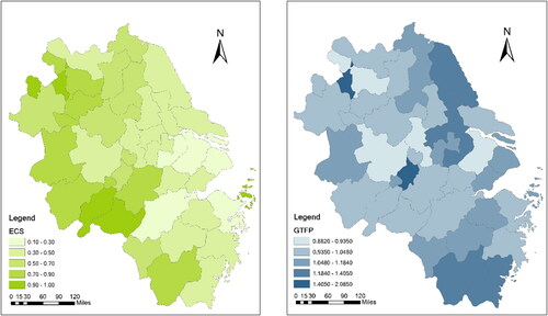
According to Figure 3, not all cities with a lower ECS have a higher GTFP. This study calculated the $\mathit{EGC}$ of 41 cities in the Yangtze River Delta city cluster from 2009 to 2019 according to Equation (1)(1) $$\begin{array}{c}D=\sqrt{C\mathrm{*}T}\\ T=\alpha U_1+\beta U_2\\ C=\frac{2\sqrt{{ES}_{it}\mathrm{*}{\mathit{GTFP}}_{it}}}{{ES}_{it}+{\mathit{GTFP}}_{it}}\end{array}$$(1) . The geographical distribution of the $\mathit{EGC}$ in each city in 2009, 2012, 2015, and 2018 is shown in Figure 4.

Figure 4. Spatial and temporal variation of.${\mathit{EGI}}_{it}$

Source: The author

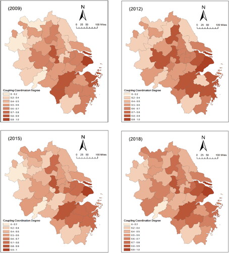
From a temporal perspective, the $\mathit{EGC}$ has a rising trend over time, indicating that the policy of emphasising green and sustainable development has been well implemented, as China is poised to change its economic development model.

From a spatial perspective, Shanghai, Nanjing, Hangzhou, Hefei, and other municipalities and provincial capitals have the highest $\mathit{EGC},$ followed by the surrounding cities and gradually spreading in all directions. However, the $\mathit{EGC}$ is significantly higher in cities located in Jiangsu and Zhejiang provinces compared to the cities in the Hefei province, indicating a clear geographical difference in the $\mathit{EGC}.$

4.2. Results of the spatial econometric model

4.2.1. Results of classical linear model regression

This study first performs a classical linear model regression of the variables on panel data (see Table 2) to facilitate the subsequent model setting, excluding the insignificant factors: traffic level ($HM$), opening level ($\mathit{FDI}$), and informatisation level ($IL$). The control variables finally determined include urban development ($UL$), knowledge intensity ($KI$), and financial development ($\mathit{RLB}$).

Table 2. Results of classical linear panel data model regression.

Variables	Coefficient	t-stat	p-value
${\mathit{PDI}}_{i,t}$	9.4516***	3.1256	0.0020
${\mathit{NGP}}_{i,t}$	0.8445***	3.3121	0.0010
${\mathit{REG}}_{i,t}$	1.4001***	2.8974	0.0021
${\mathit{PSI}}_{i,t}$	3.1215***	2.7844	0.0062
${UL}_{i,t}$	0.0121**	2.4512	0.0110
${HM}_{i,t}$	−1.2045	−1.5123	0.9812
${IL}_{i,t}$	−8.8745	−1.2132	0.5124
${KI}_{i,t}$	−3.4500**	−1.7512	0.0600
${\mathit{FDI}}_{i,t}$	4.9894	1.1324	0.8441
${\mathit{RLB}}_{i,t}$	4.1324**	2.1131	0.0311
$R^2$	0.7953
$Ad\_R^2$	0.7185

Note: ***, **, and * denote significance at the 1%, 5%, and 10% levels, respectively; the z-values are in brackets.

Source: Author's calculation.

4.2.2. Results of spatial econometric model selection

According to the test procedure provided by Anselin et al. (2008), this study first performs a Lagrange multiplier (LM) statistical test and selects a spatial econometric model based on the test results (see Table 3).

Table 3. Results of LM statistic test.

	t-Statistic	Probability
LM test no spatial lag	56.1213.35	0.000
robust LM test no spatial lag	11.3198	0.001
LM test no spatial error	42.7945	0.000
robust LM test no spatial error	6.4512	0.053
R^2		0.7955

Source: Author’s calculation.

The LM statistic test values are shown in Table 3, R²=0.7955, which is a relatively good fit. The estimated values of LM_ρ for the spatial lag model (SLM) and LM_λ for the spatial error model (SEM) reject the original hypothesis that the model does not have a spatial lag term and a spatial error term at the 1% and 5% significance levels, respectively. This proves that the spatial correlation between the observations is significant and also that the robust LM_ρ is more significant than the robust LM_λ (PSLM = 0.000 < 0.01 < PSEM = 0.053) and has a higher t-value. Therefore, a SLM should be chosen, which can be expressed as follows: (7) $$\mathrm{ }{\mathit{EGI}}_{i,t}=\rho {\sum }_{j=1}^N{W}_{ij}{\mathit{EGI}}_{i,t}+X_{i,t}\beta +u_{i,t}+v_{i,t}{X}_{i,t}={\alpha }_1{\mathit{PDI}}_{i,t}+{\alpha }_2{\mathit{NGP}}_{i,t}+{\alpha }_3{\mathit{REG}}_{i,t}{+\alpha }_4{\mathit{PSI}}_{i,t}{+\alpha }_5{UL}_{i,t}{+\alpha }_6{KI}_{i,t}{+\alpha }_7{\mathit{RLB}}_{i,t}{\mathrm{ }u}_{i,t}=c_i+{\phi }_t$$(7) (7)where $i$ = 1, 2,…, N cities; $t$ =1, 2,…, T years; ${\mathit{EGI}}_{i,t}$ is the explained variable of city $i$ in year$\mathrm{ }t;$ $X_{i,t}$ is the explanatory variable of city $i$ in year $t,$ and is expressed as Equation (7); $u_{i,t}$ is the individual specific effect of city $i$ in year $t;$ ρ is the regression coefficient of the spatial lag term; and $W_{ij}$ is the spatial weight matrix between city $i$ and city $j.$ Based on the geographical coordinates of 41 cities in the Yangtze River Delta, this study used a binary spatial adjacency matrix to determine the spatial weight matrix of the model. This study assumed that the spatial weight matrix does not vary with time $t;$ ${\beta ,\mathrm{ }{\theta }_1,\mathrm{ }{\theta }_2,\mathrm{ }\alpha }_1,{\mathrm{ }\alpha }_2,{\mathrm{ }\alpha }_3,{\mathrm{ }\alpha }_4{,\mathrm{ }\alpha }_5{,\mathrm{ }\alpha }_6,\mathit{and}{\mathrm{ }\alpha }_7$ are the parameters to be estimated; $v_{i,t}$ represents the error term of city $i$ in year $t;$ and $v_{i,t}\sim （0,{\sigma }^2）.$

The treatment of individual-specific effects $u_{i,t}$ is generally divided into fixed effects and random effects based on the correlation between $u_{i,t}$ and $X_{i,t}.$ $c_i$ and ${\phi }_t$ represent spatial fixed effects and time fixed effects, respectively. The results of the Hausman test of the SLM are shown in Table 4.

Table 4. Results of the Hausman test of the SLM.

Statistic	Degrees of freedom	Probability
48.21956	10	0.0081

Source: Author's calculation.

It was found that the P-value of the Hausman test result was less than 0.01, so the null hypothesis was accepted, and $u_{i,t}$ was regarded as a random variable with a mean of 0 and a variance of ${\sigma }^2$ to be added into the model, namely, the fixed effect was selected.

In spatial measures, fixed effects are divided into regional individual fixed effects, period fixed effects, and double fixed effects. Usually, fixed effects can be determined by comparing the fit of the spatial econometric model under the three effects or by the Likelihood Ratio (LR) test; the results of the LR test are shown in Table 5.

Table 5. Results of LR test.

Test Statistic	Statistic	Degrees of freedom	Probability
LR-test joint significance spatial fixed effects	275.1905	41	0.0015
LR-test joint significance time-period fixed effects	32.4087	10	0.0000

Source: Author's calculation.

The results show that both spatial fixed effects and temporal fixed effects were significant; therefore, individual double fixed effects were chosen.

4.2.3. Results of the spatial econometric model

Based on the test results, this study determined a panel SLM with individual double fixed effects and used a systematic generalized method of moments (GMM) approach to model regression using MATLAB R2019 software. All the variables were taken as logarithms to reduce the problem of singular values and multicollinearity. The results of the model are shown in Table 6.

Table 6. Results of individual double fixed effects panel SLM.

Variable	Coefficient	t-stat	z-probability
$ln{\mathit{PDI}}_{i,t}$	0.4513***	3.8123	0.0005
$ln{\mathit{NGP}}_{i,t}$	0.6550**	2.0651	0.0132
${\mathit{lnREG}}_{i,t}$	0.0561***	2.7231	0.0013
${\mathit{lnPSI}}_{i,t}$	0.3412***	2.7756	0.0009
$ln{UL}_{i,t}$	0.6152**	1.9880	0.0412
$ln{KI}_{i,t}$	0.1121*	2.0512	0.6781
${\mathit{lnRLB}}_{i,t}$	0.5541*	1.7564	0.0891
$\rho$	0.3650**	1.8911	0.0341
$\mathit{Nobs}$	410
$R^2$	0.7122

Note: ***, **, and * denote significance at the 1%, 5%, and 10% levels, respectively; the z-values are in brackets.

Source: Author's calculation.

The results show that the coefficients of the core explanatory variables: economic fundamentals, technological innovations, environmental regulations, and industrial structure are positive and significant at the 1% level, supporting Hypothesis 1. This phenomenon suggests that the $\mathit{EGC}$ is significantly affected by local economic development, technological innovations, environmental regulations, and industrial structure. Cities with high rates of economic development and large economies will have more financial capacity to drive the optimisation and improvement of local energy structures and more public spending to reduce pollutant emissions. Cities with solid technological innovations are more likely to promote the technological progress of industrial enterprises so that their products have the characteristics of 'high output' and meet the requirements of 'low consumption' and change the overall ECS of the city by increasing the use of clean energy and low-pollution energy. By increasing the use of clean and low-pollution energy, the overall ECS of the city will be changed, and at the same time, the GTFP will be further improved to promote coordination. Cities with strong environmental regulations will force enterprises to eliminate outdated technologies and accelerate their 'innovation compensation' by improving their technological innovations. However, scholars have found a non-linear effect of technological innovations on the ECS or GTFP through technological innovations and environmental regulations, respectively, and the GTFP through technological innovations and environmental regulations. It is the same for environmental regulations. The relationship between technological innovations and environmental regulations is also non-linear. The conclusions drawn imply that the $\mathit{EGC}$ can only be effectively increased when economic development, industrial structure, technological innovations, and environmental regulations act simultaneously. As mentioned in the Introduction, this explains why many Chinese cities have failed to improve the ECS and GTFP, either by imposing strict environmental regulations or investing heavily in technological innovations.

The results show that the other control variables selected are also significant at the 1%, 5%, and 10% significance levels, respectively, of the model $R^2$ = 0.7122, implying a good model fit. The spatial auto-correlation coefficient ρ is positive and significant at the 5% level, indicating a positive spatial spill over effect in the $\mathit{EGC}.$ As one of the most important regional development strategies in China in the past decade, the achievements made by the capital cities of the municipalities and provinces in improving the ECS and GTFP will spread rapidly to the neighbouring cities—an inevitable result of the short distance in the geographical unit. To explore the effect of the core explanatory variables on the explained variables further, a parameter decomposition of the short-term effects of the SLM was conducted, and the results are shown in Table 7.

Table 7. Parameter decomposition of short-term effects of individual double fixed effects panel SLMs.

Variable	Direct Effects	t-stat	Indirect Effects	t-stat	Total Effects	t-stat
$ln{\mathit{PDI}}_{i,t}$	0.3514	4.5612	0.0121	2.3242	0.3635	3.9412
$ln{\mathit{NGP}}_{i,t}$	0.1814	2.7842	0.0978	2.7497	0.2792	2.5611
${\mathit{lnREG}}_{i,t}$	0.5121	2.9812	−0.8712	0.7512	1.3833	4.3233
${\mathit{lnPSI}}_{i,t}$	0.4751	3.1211	0.0081	3.1512	0.4832	4.1262
$ln{UL}_{i,t}$	0.6412	1.9781	0.2122	1.4512	0.8534	2.1395
$ln{KI}_{i,t}$	0.4363	1.6987	0.1215	0.5612	0.5578	0.7589
${\mathit{lnRLB}}_{i,t}$	0.8712	1.6421	0.4512	1.9121	1.3224	1.4518

Source: Author's calculation.

The results show that a region's economic growth promotes the $\mathit{EGI}$ in the region as well as in neighbouring regions. Economic growth in a region drives the development of enterprises in that region as well as in neighbouring regions to form industrial clusters. This will, in turn, promote more $\mathrm{E}GC$ in neighbouring regions, and technological innovations and industrial structure of the cities in the region will also have a significant positive impact on the region's $\mathit{EGC}$ and the surrounding areas. Enterprises will choose to stay in the central city or spread to surrounding areas according to their development in terms of the environmental regulation intensity and industrial structure transformation. As technological innovations have spatial spill over characteristics, neighbouring regions will also improve their $\mathit{EGC}$ under the role of enterprises. More specifically, after decomposing the effects, this study found that the effect of environmental regulations on neighbourhood coordination is not significant.

4.3. Endogenous and Robustness test

4.3.1. Endogenous test

The analytical framework focuses on regressing the $\mathit{EGC}$ from four components: economic, structural, technological, and policy. However, considering that the level of economic development is an essential part of the calculation of GTFP, it may have endogeneity issues. To mitigate possible reverse causality and omitted variables between the level of economic development and the $\mathit{EGC},$ this study used the night-time lighting（$\mathit{NTL}$）data as an instrumental variable for the level of economic development in the regression. The reasons are as follows: first, the relationship between $\mathit{NTL}$ data and the GDP is close. Existing studies show that $\mathit{NTL}$ data is a good proxy for the level of local economic development, reflecting the performance of the local economic activity. Therefore, it meets the requirement of 'relevance' of the instrumental variable. Second, $\mathit{NTL}$ data does not reflect the GTFP and ECS, as it is not possible to prove whether the energy source for $\mathit{NTL}$ is fossil or clean, which also satisfies the 'homogeneity' condition of the instrumental variable.

The endogeneity results show that $\mathit{NTL}$ data, as an instrumental variable, are significantly and positively correlated with the $\mathit{EGC}.$ The instrumental variable passes the weak instrumental variable test and rejects the original unidentifiable, weak, and over-identifiable hypotheses, indicating that the instrumental variable was chosen reasonably and the test results suggest that the previous conclusions are robust. Table 8 shows the results.

Table 8. Results of the endogenous test.

Explanatory variables		${\mathit{EGI}}_{i,t}$
$\mathit{NTL}$		0.3102*** （3.6519）
Non-recognition test	Anderson canon LM statistic	8.3251***
	Cragg-Donald Wald test	8.1431***
Weak identification test	Cragg-Donald Wald test	9.0201***
Weak instrumental variable test	Anderson-Rubin Wald test	6.8716***
	Anderson-Rubin Wald test	6.4341***
	Stock-Wright LM statistic	5.2311***
Over-identification test	Sargan statistic	0.0001***

Note: ***, **, and * denote significance at the 1%, 5%, and 10% levels, respectively; the z-values are in brackets.

Source: Author's calculation.

4.3.2. Robustness test

The geographic weight matrix used is the distance inverse weight matrix, and the use of distance inverse weight evidence can better avoid the problem of economic distance, which is neglected because it judges only the proximity of geographic units compared to the binary adjacency weight matrix. However, for the Yangtze River Delta urban agglomeration, the $\mathit{EGC}$ depends on geographical distance. It is influenced by the closeness of economic ties between different regions. For example, Nanjing and Yangzhou, which belong to the Jiangsu province, are closer to Hefei in the Anhui province, but Shanghai influences them more in terms of economic growth, technological innovations, and environmental regulations. Therefore, this study used the economic weight matrix $W_{ij}^e.$ After replacing the geographic weight matrix, the model was changed from a double fixed model to an individual fixed-effects model, and the rest of the model settings remained unchanged; the results are shown in Table 9.

Table 9. Results of the robustness test.

Variable	Coefficient	t-stat	z-probability
$ln{\mathit{PDI}}_{i,t}$	0.3512***	3.4511	0.0008
$ln{\mathit{NGP}}_{i,t}$	0.5612***	3.3245	0.0009
${\mathit{lnREG}}_{i,t}$	0.0784***	2.0347	0.0312
${\mathit{lnPSI}}_{i,t}$	0.6512**	1.7546	0.0712
$ln{UL}_{i,t}$	0.3218**	1.6881	0.0598
$ln{KI}_{i,t}$	0.1210*	1.7456	0.0521
${\mathit{lnRLB}}_{i,t}$	0.2671*	1.6231	0.0701
$\rho$	0.2037***	3.0121	0.0011
$\mathit{Nobs}$	410
$R^2$	0.7512

Note: ***, **, and * denote significance at the 1%, 5%, and 10% levels, respectively; the z-values are in brackets.

Source: Author's calculation.

The robustness results show that there is still a relatively significant positive spatial correlation between the ECS and GTFP and that each core explanatory variable remains significant at the 1% level, indicating the robustness of regression results.

5. Conclusion

This study constructed a theoretical framework that influences the $\mathit{EGC}$ through theoretical analysis and used spatial panel data of 41 cities in the Yangtze River Delta urban agglomeration from 2009 to 2019 to test the spatial influence of economic development, technological innovations, environmental regulations, and industrial structure on the $\mathit{EGC}$ by constructing an SLM.

The core findings are as follows: (a) The $\mathit{EGC}$ has more obvious spatial and temporal evolution characteristics. From a temporal perspective, the $\mathit{EGC}$ of each city in the Yangtze River Delta urban agglomeration increases year by year, indicating that the existing ECS of each city is continuously optimised and can effectively promote the improvement of local GTFP. From a regional perspective, cities with higher $\mathit{EGC}$ are mainly municipalities directly under the Central government, provincial capitals, and cities with a large scale and high economic level, which confirms the findings of Chen et al. (2020) regarding the promotion of economic growth in developing countries using renewable energy above the threshold. In contrast, cities with a lower $\mathit{EGC}$ are mainly those with industrial production as the core economic activity, high energy consumption, and low economic development level. This phenomenon indicates that the $\mathit{EGC}$ has prominent spatial heterogeneity characteristics. (b). The $\mathit{EGC}$ has spatial spill over effects. Economic development, technological innovations, environmental regulations, and industrial structure significantly improve the $\mathit{EGC}$ development index. This conclusion has been confirmed by other scholars in similar studies on the spatial influences of the ECS and GTFP (Lee et al., 2022; Wang et al., 2020; Zhou et al., 2020;). This improvement is reflected in the region's influence on itself and on neighbouring regions, with the effect of environmental regulations on local and neighbourhood coordination being insignificant.

Based on the conclusions and findings, this study argues that the spatial auto-correlation of the $\mathit{EGC}$ means that central cities should take more responsibility for the improvement of the $\mathit{EGC},$ thereby increasing the spatial spill-over effect and driving the simultaneous improvement of neighbouring cities. In the specific practice of local governments, as this study finds that technological innovations and industrial structure show significant spill-over effects in the spatial interaction process of the $\mathit{EGC},$ central cities should drive the development of the $\mathit{EGC}$ in neighbouring cities by strengthening local technological innovations and optimising the industrial structure because they have better capital and intellectual factor endowments. In contrast, neighbouring cities should pay more attention to their $\mathit{EGC}$ as the spatial indirect effects of environmental regulations are not significant. Therefore, neighbouring cities should focus more on their environmental regulation policies, as they cannot rely on the spatial influence of the central city.

Future research should focus on the relationship between energy structure and the GTFP. The ECS is only a part of the energy structure, which also includes energy endowment, energy production volume, and energy import and export volumes. The relationship between these factors and the GTFP is not yet clear, and research on the relationship between energy structure and the GTFP can be enriched via the expansion of the scope of research.

Disclosure statement

The authors report there are no competing interests to declare.

Additional information

Funding

This work was supported by the Fundamental Research Funds for the Central Universities (21lzujbkyjh012)

References

- Anselin, L., Le Gallo, J., & Jayet, H. (2008). Spatial panel econometrics. In L. Mátyás, & P. Sevestre (Eds.), The econometrics of panel data (pp. 625–660). Springer.
- Bakirtas, T., & Akpolat, A. G. (2018). The relationship between energy consumption, urbanization, and economic growth in new emerging-market countries. Energy, 147, 110–121. https://doi.org/10.1016/j.energy.2018.01.011
- Central Committee of the CPC and the State Council. (2021, November 11). Opinions of the Central Committee of the CPC and the State Council on Carbon Dioxide Peaking and Carbon Neutrality in full and faithful implementation of the new development philosophy. Retrieved from. http://english.www.gov.cn/archive/statecouncilgazette/202111/11/content_WS618d0192c6d0df57f98e4d0d.html
- Chen, C., Pinar, M., & Stengos, T. (2020). Renewable energy consumption and economic growth nexus: Evidence from a threshold model. Energy Policy, 139, 111295. https://doi.org/10.1016/j.enpol.2020.111295
- Dabbous, A., & Tarhini, A. (2021). Does sharing economy promote sustainable economic development and energy efficiency? Evidence from OECD countries. Journal of Innovation & Knowledge, 6(1), 58–68. https://doi.org/10.1016/j.jik.2020.11.001
- Du, K., Cheng, Y., & Yao, X. (2021). Environmental regulation, green technology innovation, and industrial structure upgrading: The road to the green transformation of Chinese cities. Energy Economics, 98, 105247. https://doi.org/10.1016/j.eneco.2021.105247
- Feng, T., Sun, L., & Zhang, Y. (2009). The relationship between energy consumption structure, economic structure and energy intensity in China. Energy Policy, 37(12), 5475–5483. https://doi.org/10.1016/j.enpol.2009.08.008
- Huang, C., Zhang, Z., Li, N., Liu, Y., Chen, X., & Liu, F. (2021). Estimating economic impacts from future energy demand changes due to climate change and economic development in China. Journal of Cleaner Production, 311, 127576. https://doi.org/10.1016/j.jclepro.2021.127576
- Lee, C. C., Zeng, M., & Wang, C. (2022). Environmental regulation, innovation capability, and green total factor productivity: New evidence from. China. Environmental Science and Pollution Research International, 29, 39384–39399. https://doi.org/10.1007/s11356-021-18388-0
- Luan, B., Zou, H., Chen, S., & Huang, J. (2021). The effect of industrial structure adjustment on China's energy intensity: Evidence from linear and nonlinear analysis. Energy, 218, 119517. https://doi.org/10.1016/j.energy.2020.119517
- Maji, I. K., Sulaiman, C., & Abdul-Rahim, A. S. (2019). Renewable energy consumption and economic growth nexus: A fresh evidence from West. Africa. Energy Reports, 5, 384–392. https://doi.org/10.1016/j.egyr.2019.03.005
- Murad, M. W., Alam, M. M., Noman, A. H. M., & Ozturk, I. (2019). Dynamics of technological innovation, energy consumption, energy price and economic growth in Denmark. Environmental Progress & Sustainable Energy, 38(1), 22–29. https://doi.org/10.1002/ep.12905
- Oh, D. H. (2010). A global Malmquist-Luenberger productivity index. Journal of Productivity Analysis, 34(3), 183–197. https://doi.org/10.1007/s11123-010-0178-y
- Pegkas, P. (2020). The impact of renewable and non-renewable energy consumption on economic growth: The case of Greece. International Journal of Sustainable Energy, 39(4), 380–395. https://doi.org/10.1080/14786451.2019.1700261
- Porter, M. E., & Van der Linde, C. (1995). Toward a new conception of the environment-competitiveness relationship. Journal of Economic Perspectives, 9(4), 97–118. https://doi.org/10.1257/jep.9.4.97
- Ren, S., Hao, Y., Xu, L., Wu, H., & Ba, N. (2021). Digitalization and energy: How does internet development affect China's energy consumption? Energy Economics, 98, 105220. https://doi.org/10.1016/j.eneco.2021.105220
- Saint Akadiri, S., Alola, A. A., Akadiri, A. C., & Alola, U. V. (2019). Renewable energy consumption in EU-28 countries: Policy toward pollution mitigation and economic sustainability. Energy Policy, 132, 803–810. https://doi.org/10.1016/j.enpol.2019.06.040
- Sharma, G. D., Tiwari, A. K., Erkut, B., & Mundi, H. S. (2021). Exploring the nexus between non-renewable and renewable energy consumptions and economic development: Evidence from panel estimations. Renewable and Sustainable Energy Reviews, 146, 111152. https://doi.org/10.1016/j.rser.2021.111152
- Shen, L., Fan, R., Wang, Y., Yu, Z., & Tang, R. (2020). Impacts of environmental regulation on the green transformation and upgrading of manufacturing enterprises. International Journal of Environmental Research and Public Health, 17(20), 7680. https://doi.org/10.3390/ijerph17207680
- Shen, N., Liao, H., Deng, R., & Wang, Q. (2019). Different types of environmental regulations and the heterogeneous influence on the environmental total factor productivity: Empirical analysis of China's industry. Journal of Cleaner Production, 211, 171–184. https://doi.org/10.1016/j.jclepro.2018.11.170
- Streimikis, J., & Saraji, M. K. (2021). Green productivity and undesirable outputs in agriculture: A systematic review of DEA approach and policy recommendations. Economic Research-Ekonomska Istraživanja, 1–35. https://doi.org/10.1080/1331677X.2021.1942947
- Töbelmann, D., & Wendler, T. (2020). The impact of environmental innovation on carbon dioxide emissions. Journal of Cleaner Production, 244, 118787. https://doi.org/10.1016/j.jclepro.2019.118787
- Tomal, M. (2021). Evaluation of coupling coordination degree and convergence behaviour of local development: A spatiotemporal analysis of all Polish municipalities over the period 2003–2019. Sustainable Cities and Society, 71, 102992. https://doi.org/10.1016/j.scs.2021.102992
- Tone, K. (2001). A slacks-based measure of efficiency in data envelopment analysis. European Journal of Operational Research, 130(3), 498–509. https://doi.org/10.1016/S0377-2217(99)00407-5
- Tseng, S. W., Chen, Y. Y, & the National Taiwan Ocean University, Keelung City 202, Taiwa. (2021). How did the changes in industrial and energy structure influence energy consumption in Shandong. Journal of Clean Energy Technologies, 9(1), 1–11. https://doi.org/10.18178/JOCET.2021.9.1.524
- UNEP Copenhagen Climate Centre. (2021). Emissions gap report 2021. Retrieved from https://www.unep.org/resources/emissions-gap-report-2021.
- Wang, C., Geng, L., & Rodríguez-Casallas, J. D. (2021). How and when higher climate change risk perception promotes less climate change inaction. Journal of Cleaner Production, 321, 128952. https://doi.org/10.1016/j.jclepro.2021.128952
- Wang, H., Cui, H., & Zhao, Q. (2021). Effect of green technology innovation on green total factor productivity in China: Evidence from spatial Durbin model analysis. Journal of Cleaner Production, 288, 125624. https://doi.org/10.1016/j.jclepro.2020.125624
- Wang, K. L., Pang, S. Q., Ding, L. L., & Miao, Z. (2020). Combining the biennial Malmquist–Luenberger index and panel quantile regression to analyze the green total factor productivity of the industrial sector in China. The Science of the Total environment, 739, 140280.
- Wang, X., Zhang, Y., & Chen, N. (2021). Modern service industry agglomeration and its influencing factors: Spatial interaction in Chinese cities. Economic Research-Ekonomska Istraživanja, 1–20.
- Wang, Z., Xia, C., & Xia, Y. (2020). Dynamic relationship between environmental regulation and energy consumption structure in China under spatiotemporal heterogeneity. The Science of the Total environment, 738, 140364.
- Xie, F., Zhang, B., & Wang, N. (2021). Non-linear relationship between energy consumption transition and green total factor productivity: A perspective on different technology paths. Sustainable Production and Consumption, 28, 91–104. https://doi.org/10.1016/j.spc.2021.03.036
- Xie, R., Fu, W., Yao, S., & Zhang, Q. (2021). Effects of financial agglomeration on green total factor productivity in Chinese cities: Insights from an empirical spatial Durbin model. Energy Economics, 101, 105449. https://doi.org/10.1016/j.eneco.2021.105449
- Xing, L., Xue, M., & Hu, M. (2019). Dynamic simulation and assessment of the coupling coordination degree of the economy–resource–environment system: Case of Wuhan City in China. Journal of Environmental management, 230, 474–487.
- Xu, X., & Lee, L. F. (2019). Theoretical foundations for spatial econometric research. Regional Science and Urban Economics, 76, 2–12. https://doi.org/10.1016/j.regsciurbeco.2018.04.002
- Yang, M., Yuan, Y., Yang, F., & Patino-Echeverri, D. (2021). Effects of environmental regulation on firm entry and exit and China's industrial productivity: A new perspective on the Porter Hypothesis. Environmental Economics and Policy Studies, 23(4), 915–944. https://doi.org/10.1007/s10018-021-00310-0
- Zafar, M. W., Shahbaz, M., Sinha, A., Sengupta, T., & Qin, Q. (2020). How renewable energy consumption contribute to environmental quality? The role of education in OECD countries. Journal of Cleaner Production, 268, 122149. https://doi.org/10.1016/j.jclepro.2020.122149
- Zeng, S., Su, B., Zhang, M., Gao, Y., Liu, J., Luo, S., & Tao, Q. (2021). Analysis and forecast of China's energy consumption structure. Energy Policy, 159, 112630. https://doi.org/10.1016/j.enpol.2021.112630
- Zhang, X. H., Zhang, R., Wu, L. Q., Deng, S. H., Lin, L. L., & Yu, X. Y. (2013). The interactions among China's economic growth and its energy consumption and emissions during 1978–2007. Ecological Indicators, 24, 83–95. https://doi.org/10.1016/j.ecolind.2012.06.004
- Zheng, W., & Walsh, P. P. (2019). Economic growth, urbanization and energy consumption—A provincial level analysis of China. Energy Economics, 80, 153–162. https://doi.org/10.1016/j.eneco.2019.01.004
- Zhou, H., Qu, S., Wu, Z., & Ji, Y. (2020). A study of environmental regulation, technological innovation, and energy consumption in China based on spatial econometric models and panel threshold models. Environmental Science and Pollution Research international, 27(30), 37894–37910.
- Zhou, R., Zhang, Y., & Gao, X. (2021). The spatial interaction effect of environmental regulation on urban innovation capacity: Empirical evidence from China. International Journal of Environmental Research and Public Health, 18(9), 4470. https://doi.org/10.3390/ijerph18094470