
 ?Mathematical formulae have been encoded as MathML and are displayed in this HTML version using MathJax in order to improve their display. Uncheck the box to turn MathJax off. This feature requires Javascript. Click on a formula to zoom.
Abstract
This paper investigates the time-varying lead-lag relationship between CSI 300 index futures and the cash index at intraday and daily frequencies under different market conditions, which is crucial in the price discovery research but rarely examined by the literature. Using a new method that is based on dynamic time warping and can capture the dynamic lead-lag relationship up to the intraday level, we find that index futures tend to lead the cash index by 0–5 minutes but it occasionally lags the cash index, and this relationship is variably affected by factors according to market conditions. Specifically, at both of the intraday and daily frequencies, the lead of index futures decreases with market volatility and the relative intensity of trading activity of index futures. The results also unveil the asymmetric effects of overnight information from the cash market on the lead times of both index futures and the cash index at a daily frequency. Moreover, the synchronization of trading hours strengthened the link between the two markets. These results have significant implications for price discovery in these markets.
1. Introduction
The lead-lag relationship between index futures and the cash index reflects the relative speed of incorporating new information in the two markets, and more importantly, its time-varying characteristics have significant implications for the dynamic process of price discovery and risk management in an ever-changing market. A vast amount of literature, discussed in greater detail in the next section, has investigated the lead-lag relationship. However, far less clear are the time-varying characteristics of the lead-lag relationship, especially under different market conditions. We aim to fill this gap in the literature by estimating the dynamic lead-lag relationship with a new measurement based on dynamic time warping (DTW) (Ma et al., Citation2022) and investigating its time-varying characteristics by analysing the effects of possible market microstructure factors on this relationship under different market conditions distinguished by perceptually important points (PIPs).
It will be of great value to examine this relationship in China for several reasons. First, since introduced on April 2010, CSI 300 index futures have rapidly became one of the most active futures contracts in the world. The CSI 300 index that consists of major blue-chip stocks listed on the Shanghai and Shenzhen Stock Exchanges is generally considered as an indicator of the Chinese stock market. Using the past 11 years of data on CSI 300 index futures and the underlying index, we are able to investigate how the lead-lag relationship between the two markets and their price discovery performance behaves under different market conditions.
Furthermore, the characteristics of the lead-lag relationship between Chinese cash and index futures markets are quite different from other international markets in the following respects. First, the Chinese stock market trades with a special mechanism called “T + 1” that prohibits investors from selling shares bought on the current day until the next trading day (Qiao & Dam, Citation2020). Second, short-selling is severely restricted in the Chinese stock market, and there are no other tools such as individual stock futures and options to hedge the downward risks of specific stocks. Third, high barriers to trading the index futures such as minimum account size requirements and other personal experience result in very few individual investors participating in the index futures market.
In addition, there is no consensus on which market (i.e., the index futures market or the cash market) leads (Judge & Reancharoen, Citation2014), especially in the context of China (e.g., He et al., Citation2020; Wang et al., Citation2017). There is also little empirical evidence about the characteristics of the intraday lead-lag structure and/or price discovery of the two markets under different market conditions.
Overall, investigating this relationship in the Chinese markets could provide more insights into price discovery and the design of the trading mechanism, which would also provide a reference for other international markets.
Our paper extends the existing literature in two respects. First, we document a dynamic lead-lag relationship at the intraday and daily frequency. This relationship could be asymmetric at daily frequency. Second, we provide empirical evidence on how the influences of market volatility and the relative intensity of trading activity at the intraday and daily frequency as well as the influences of overnight information at a daily frequency on the performance of price discovery among index futures and the cash index markets vary/accord under different market conditions. In more detail, our analysis leads to several noteworthy findings.
Although CSI 300 index futures usually lead the cash index by 0–5 minutes regardless of market conditions, it also occasionally lags the cash index. For example, from 2010 to 2021, the index futures lead the cash index at a one-minute interval in 80.90% of cases.
The intraday lead-lag structure exhibits different patterns under different scenarios and in different periods. For example, when the market is crashing, the index futures lead the cash index to a greater extent and with a higher probability than in other periods, suggesting that index futures play an important price discovery role during this period.
At a daily interval, the lead time of index futures or the cash index decreases with the relative volume of index futures, market volatility, and the synchronization of trading hours, indicating a tighter correlation between the two markets.
However, the overnight information, on the one hand, imposes different impacts on the lead times of index futures and those of the cash index depending on market conditions, e.g., positive overnight information would increase the lead time of index futures in the Bull period but decrease it in the Rally period. On the other hand, the overnight information also has “leverage” effects on their lead times, e.g., the effect of positive overnight information on the lead times of the cash index is much larger than those of negative overnight information in the Bull period.
The remainder of the paper proceeds as follows. Section 2 reviews the literature on the lead-lag relationship. Section 3 demonstrates how to estimate lead-lag times using DTW and how to identify different periods using PIPs and sets forth our research method. Section 4 describes the data used for our investigation, and Section 5 provides the empirical results. Section 6 concludes the paper.
2. Literature review
In perfectly efficient markets, new information is incorporated simultaneously and completely by stock index futures and the underlying cash index, leading to a theoretical synchronicity between them. However, in the real world, an empirical lead-lag relationship between index futures and the cash index is observed due to the existence of frictions such as trading costs, nonsynchronous trading and barriers to short selling (Chan, Citation1992). Because futures markets can assimilate new information more quickly than cash markets due to their leverage, high intensity of trading activity, low trading cost and easy access to short selling (Tse, Citation1999), they are always found to lead cash markets or play a predominant role in price discovery in many international markets (e.g., Alemany et al., Citation2020; Chan, Citation1992; Kavussanos et al., Citation2008; Wang et al., Citation2017), whereas there is evidence that the futures markets lag cash markets (e.g., Judge & Reancharoen, Citation2014; Ren et al., Citation2019; Y.-H. Yang & Shao, Citation2020 ). Furthermore, in some countries, especially China, the empirical findings of the dominant market for price discovery are mixed. For example, Wang et al. (Citation2017) and Miao et al. (Citation2017) suggest that the index futures market dominates price discovery, while J. Yang et al. (Citation2012) and Zhou et al. (Citation2021) argue that the cash market plays a leading role in the price discovery process. Additionally, some of the studies mentioned above examine the time-varying characteristics of the lead-lag relationship between index futures and the cash index.
Furthermore, various approaches including GARCH models (Zhong et al., Citation2004), Granger causality analysis (T. Jiang et al., Citation2019), regression approaches (Chan, Citation1992), wavelet analysis (In & Kim, Citation2006) and optimal thermal causal path (Wang et al., Citation2017) have been adopted to examine the lead-lag relationship between the two markets, but few of them can estimate the exact lead-lag time at high frequency such as at a one-minute interval. Accordingly, Ma et al. (Citation2022) propose a nonparametric measurement of the lead-lag relationship between index futures and the cash index based on DTW, which could capture the complex and dynamic local lead-lag structure, and this approach is used in our analysis.
A number of studies have investigated the factors that drive the different lead-lag relationships between index futures and the cash index. Some argue that trading volume and turnover are critical determinants of the lead–lag relationship (e.g., Chung et al., Citation2011; He et al., Citation2020 ), while others suggest that information or trading costs could drive the lead–lag relationship by delaying the process of information incorporation (e.g., Fleming et al., Citation1996; Huang et al., Citation2021). Moreover, Chan (Citation1992) provide evidence that market-wide information could contribute to a greater degree of leading by index futures. L. Jiang et al. (Citation2001) find that lifting short-selling restrictions could reduce leading role of index futures in the lead-lag relationship in Hong Kong. C.-B. Lin et al. (Citation2018) indicates that investor sentiment also has a significantly negative impact on the short-run leading role of futures markets.
3. Methodology
3.1. Measures of lead-lag times
We estimate the lead-lag times using the method developed by Ma et al. (Citation2022) based on DTW. DTW is wildly used in analysing the similarity of time series data in various areas (e.g., Myers et al., Citation1980; Tsinaslanidis & Kugiumtzis, Citation2014)and is extremely efficient because it allows “elastic” transformation of time series (Senin, Citation2008). From a dynamic programming process, DTW obtains a warping path that minimizes the cumulative distance between the observations of two series. Accordingly, Zoumpoulaki et al. (Citation2015) apply this path to measure latency by mapping the observations of two series because DTW allows the researcher to quantify the changes in latency across all the data points in a region rather than just one. Ito and Sakemoto (Citation2020) propose multinomial dynamic time warping (MDTW) to analyse the lead-lag relationship between currency pairs using nonsynchronous and vast data. Recently, Ma et al. (Citation2022) utilize DTW to detect the lead-lag structure due to its advantages in dealing with a complex and dynamic local lead-lag structure, which exactly corresponds with our needs.
We then briefly introduce how to estimate the lead-lag structure with an approach based on DTW. Given one-minute log-return series of the cash index and that of the index futures
in a trading day, DTW first calculates the pairwise Euclidean distance
and then iteratively constructs the cumulative distance matrix
by
with
and
The warping path
starts from
and ends at
denotes that rj and qi are matched, indicating they reflect the same signal. Each movement on the warping path is limited to the right, up or diagonal with only one step.
We assume that yj is mapped with (
) observation(s) of X denoted by
where
The lead-lag times (in minutes) for yj can be defined by
(1)
(1)
where i + h and j are the ordinal number of minutes for
and yj, respectively. Notably, a positive (negative) PLLj indicates that Y leads (lags) X at observation j.
The daily average lead-lag time (in minutes) for Y is given by
(2)
(2)
where
is defined by Equationequation (1)
(1)
(1) for day t. Again, a positive (negative) DLLt indicates that Y leads (lags) X on day t.
3.2. Identification of different market periods
To identify different market periods such as the Bull and Bear periods, we employ PIPs, a time-series data mining tool, which is constructed to identify the significant points that have the greatest influence on the shape of price time series (F. L. K. Chung et al., Citation2001). Namely, PIPs are effective at identifying structural changes. Park et al. (Citation2010) argue that PIPs are superior to the SAX (J. Lin et al., Citation2003) in representing the movement shape of time series. In fact, PIPs are the inflection points of time series. We could use them to identify market periods by detecting inflection points and then distinguishing the periods visually.
The first and the last observations are the first two PIPs characterized by the algorithm. The next PIP is the observation that has the maximum distance to the first two PIPs. The fourth PIP is the observation with the greatest distance to its adjacent PIPs that are either the first and second PIPs or the second and third PIPs. This process stops when the required number of PIPs is found. In our analysis, we assume there are seven PIPs in total.
Let be the futures price time series of length m and two adjacent PIPs ft and
To simplify the algorithm, we only consider the Euclidean distance when calculating the distance for the intermediate point
for
(3)
(3)
Then the new PIP point is the one with the maximum distance
3.3. Examination of factors
The factors that may affect the lead-lag relationship between the cash index and the index futures are tested at two frequencies—daily and intraday. On the one hand, we test the effects of intraday market trading activities such as index returns, volatility, volume, and futures volume on the lead-lag relationship in a 30-minute interval. The volatility in a 30-minute interval is the standard deviation of one-minute returns for the cash market. We first calculate the average lead-lag times of the index futures in 30-minute intervals using the estimated lead-lag times for each minute within each day. We then calculate the average lead-lag times of different quintiles based on the ranking of the variables of market trading activities, namely,index returns, volatility, volume, and futures volume. Then we can test their impacts based on the differences between (the average) lead-lag times of quintile 1 and quintile 5.
On the other hand, we further examine factors at a daily interval with ordinary least squares (OLS) regression:
(4)
(4)
where ϵ is the error term, and subscript t represents the period. The main variables are as follows.
In this regression, Leadlag represents the lead-lag times of index futures to the cash index when we assume the lead-lag relationship between the two markets is symmetric or either the lead times of index futures or that of the cash index if we assume that the lead-lag relationship is asymmetric.
VolumeRatio denotes the ratio of trading volume (RMB) for the index futures market to that of the spot market in natural logarithm. It measures the relative trading intensities in the two markets.
Volatility denotes the daily realized volatility (RV) of the cash market calculated by 5-minute returns in natural logarithm, which is proposed by Andersen and Bollerslev (Citation1998) as a measure of integrated variance and converges in probability to the quadratic variation as the time intervals between observations become infinitely small (Andersen et al., Citation2003).
Overnight denotes the overnight return (in percent) for the cash market calculated as 100 times the difference between logarithmic opening price and logarithmic closing price of the last day following Hendershott et al. (Citation2020), and — is the absolute value of Overnight. By conjoint analysis of the coefficients (β3 and β4) of these two variables, we can examine the asymmetric effects of positive and negative overnight information and their “leverage effects”Footnote1 on the lead-lag relationship between index futures and the cash index.
Synch is a dummy variable equal to one if the date is after January 1, 2016, denoting whether the index futures market and the cash market are traded synchronously. As reported in the relevant regulatory documents, the regular trading hours of the Chinese index futures market were 9:15 am–11:30 am and 13:00 pm–15:15 pm, implying it opened (closed) 15 minutes earlier (later) than the stock market. However, since January 1, 2016, the trading hours of index futures market have been the same as those of the stock market.
4. Data
The CSI 300 index (in short, the cash index) consists of the 300 largest firms listed on the Shanghai and Shenzhen stock exchanges, constituting approximately three-fifths of total market capitalization of the two stock markets, and is generally considered a measure of the overall performance of China A-share market. CSI 300 index futures (in short, the index futures), launched on April 16, 2010, is the first index futures product in China.
The one-minute prices of the cash index and CSI 300 index futures from April 16, 2010, to May 31, 2021, are both obtained from the Wind Database. The continuous price series of the stock index futures is constructed with the nearby contract, which is usually the most heavily traded contract. The 5-minute, 30-minute and daily prices are computed from the one-minute closing prices for the cash index. Since there were extended trading hours for the index futures market compared to the cash market before 2016, we drop the data covering extended trading hours for the index futures market during this time. Thus, there are 240 one-minute observations of price series of both the cash index and index futures each day. The log-return is calculated by taking the first differences of the log-prices, and the lead-lag times for one-minute log-return series are estimated separately for each day. Our sample ultimately contains 239 one-minute returns of both the cash index and the index futures each day and covers 2,703 days.
Panel A of reports the summary statistics for the two returns and the estimated results in one-minute intervals. The one-minute returns of index futures and the cash index are −0.019 basis points (bps) and 0.040 bps on average, respectively. The standard deviation of the futures is larger than that of the cash index, and their large standard deviations imply that their returns are both volatile at intraday frequency on average. Index futures lead the cash index by 0.731 minutes on average at a one-minute interval.
Table 1. Summary statistics.
Summary statistics for variables in 30-minute intervals are reported at Panel B of . Index futures lead the cash index by 0.679 minutes on average at a 30-minute interval. The average volume for index futures is larger than that for the cash index because futures are traded with margin but not the value of the contract.
Panel C of reports the summary statistics for the variables at daily frequency. Index futures and the cash index, on average, lead to each other by 1.978 and 2.199 minutes when they are leading, respectively. The trading volume for index futures is approximately 2.5 times that for the cash index because index futures are traded with margin on contract while the cash index is traded with the value of shares. The average volatility for the cash market is 1.387%. The average overnight return for the cash market is negative, which is consistent with prior findings reported by Qiao and Dam (Citation2020). On average, Synch equals to 0.487, indicating that the number of days with asynchronous trading hours for the two markets is more than the number of days with synchronous trading hours in our sample.
5. Empirical results
5.1. Statistic analysis of lead-lag times
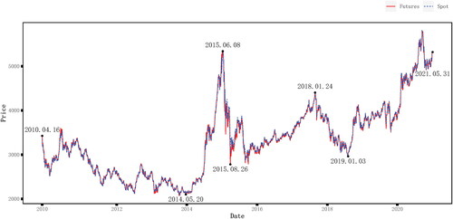
We first obtain seven PIPs on the index futures throughout the full sample period () and select four representative subsample periods: Bear (from April 16, 2010, to May 20, 2014, and from January 24, 2018, to January 3, 2019), Bull (from January 3, 2019, to May 31, 2021, and from January 3, 2019, to May 31, 2021), Crash (from June 8, 2015, to August 26, 2015) and Rally (from May 20, 2014, to June 8, 2015).
Figure 1. PIPs of the CSI 300 index futures.
Source: authors’ creation.
To put things into perspective, we partition the lead-lag times of the index futures into one-minute intervals after dropping those synchronous cases (i.e., PLL = 0) and calculate the proportions of each group for different periods (). Following the definition of outliers in Wang et al. (Citation2017), we find that most PLL values are between −10 and 10. Therefore, we only show the PLL values between −10 and 10 in the histogram.Footnote2 Throughout the sample period, the index futures lead the cash index by less than 5 minutes () for approximately 75.98% of the entire sample, which is consistent with Wang et al. (Citation2017).
Table 2. The proportion of estimated lead-lag times.
The index futures lead the cash index (as shown in the last row of ) most of the time, while lead probabilities for index futures are less than that in Wang et al. (Citation2017). There are also a few cases (less than 20% of cases) in which the cash index leads the index futures at a one-minute frequency. These results indicate that the index futures market plays the primary role in the price discovery progress regardless of the market conditions.
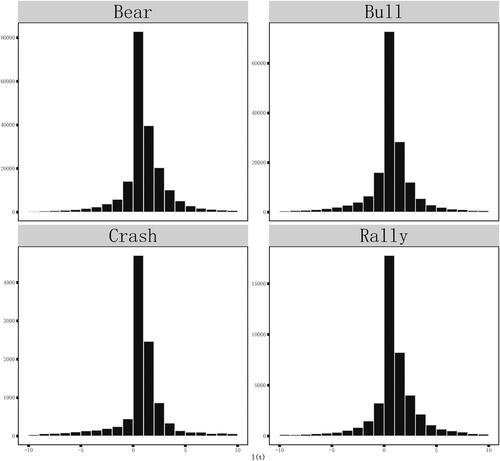
Consistent with , shows that the PLL exhibits similar patterns in different periods, i.e., the index futures lead the cash index by less than 5 minutes most of the time. The index futures lag the cash index by less than 5 minutes for most of the lagging time.
Figure 2. Histogram of intraday lead-lag times of logarithmic return of CSI 300 index futures in different subsample period.
This figure displays the histogram of intraday lead-lag times (i.e., PLL) of logarithmic return of CSI 300 index futures for four subsamples including the Bear (from April 16, 2010 through May 20, 2014 and from January 24, 2018 through January 3, 2019), the Bull (from August 26, 2015 through January 24, 2018 and from January 3, 2019 through May 31, 2021), the Crash (from June 8, 2015 through August 26, 2015) and the Rally (from May 20, 2014 to June 8, 2015). The histogram only includes the PLL between -10 minutes to 10 minutes without PLL equal to 0.
Source: authors’ creation.
5.2. At intraday frequency
5.2.1. Intraday lead-lag relationship under bad news or good news
To examine whether the lead-lag relationship exhibits different intraday patterns under different scenarios, we calculate the average lead-lag times of the index futures in 30-minute intervals using the lead-lag times for each minute estimated within each day. Following Chan (Citation1992), who argues that the 30-minute interval is proper because it not only allows the information effect to influence the lead-lag relationship of some observations but also can avoid many different bits of information, we choose 30 minutes as the appropriate interval length for analysing the intraday dynamics of the lead-lag relationship.
We first examine whether the lead-lag relationship between the cash index and index futures differs under good news and bad news by stratifying 30-minute intervals into five quintiles based on the ranking of the cash index returns (Chan, Citation1992). The return in each 30-minute interval is calculated by the opening price for the first minute and the closing price for the last minute of that interval. Quintile 1 is the group of intervals with the lowest returns of the cash index, implying that there is bad news in the market. Quintile 5 is the group of intervals with the highest returns of the cash index, implying that there is good news in the market. As the returns of the cash index and the index futures are highly correlated and news about individual stock mainly influences the price of that stock and the cash index, we only consider different news about the stock market.
The average lead-lag times in 30-minute intervals of the index futures for different quintiles are calculated and reported in . The index futures lead the cash index across all return quintiles and all periods but especially in the Crash period, when the market is characterized by volatility. Thus, the index futures tend to assimilate information more quickly and play a more important role in the price discovery process when market is volatile and experiencing a crash. However, in Bull periods, the lead of index futures is less than that in other periods, implying a more contemporaneous relationship between the two markets. The last row (H-L) of shows that there are no significant differences in lead-lag relations under good news and under bad news.
Table 3. The lead-lag relationship under bad news and good news.
5.2.2. Intraday lead-lag relationship under different market volatilities
We next examine whether the lead-lag relationship between index futures and the cash index differes under different market volatilities. Since the CSI 300 index consists of the most liquid and largest stocks of China’s A-share stock market, its volatility can be a direct proxy for the volatility of the market. The 30-minute intervals are stratified into five quintiles based on the ranking of the volatility of the cash index return in that interval. The volatility in each 30-minute interval is measured as the standard deviation of logarithmic returns for every minute of that interval. Quintile 1 is the group of intervals with the lowest volatility of the cash index return, while quintile 5 is the group of intervals with the highest volatility of the cash index return.
reports the lead-lag relationship under different volatilities of the cash market. It is clear that index futures lead the cash index across almost all volatility quintiles and all periods except during periods of extreme market volatility (i.e., quintile 5 of the Crash period). Moreover, the lead of index futures significantly decreases with volatility as shown in the last row of for almost all periods except the Bear period, which conflicts with Chen et al. (Citation2016) who find that S&P 500 index futures contribute to the price discovery progress more than the ETF in the high-volatility sub-period. This could be resulted by the difference between the Chinese and U.S. index futures markets. As we know, investors have to meet high requirements to trade index futures in China such as of minimum account size requirements (at least 500,000 RMB) and other personal experience, while it is easier and cheaper to trade index futures in the U.S. Therefore, the price discovery performance of index futures under a high-volatility scenario is better in the U.S. than in China.
Table 4. The lead-lag relationship under different market volatility.
5.2.3. Intraday lead-lag relationship under different intensities of trading activity
Additionally, we examine whether the lead-lag relationship is different under different intensities of trading activity, which is proxied by the sum of trading volumes for every minute of that interval. The 30-minute intervals are first stratified into five quintiles based on the ranking of the trading volume of the cash index in that interval. Quintile 1 is the group of intervals with the lowest trading volume of the cash index, while quintile 5 is the group of intervals with the highest trading volume of the cash index. Then, within each group, intervals are further divided into five subgroups based on the ranking of the trading volume of index futures in that interval. Therefore, each 30-minute interval is allocated to one of the 25 subgroups for each period.
shows the index futures results for groups with low and high trading volumes of index futures and the cash index in China, which are not consistent with results obtained for the U.S. (Chan, Citation1992). In general, an increasing intensity of trading activity in the cash market significantly negatively influences the lead time of index futures when the futures market is inactive, while a different intensity of trading activity in the cash market does not affect the lead-lag time of index futures when the index futures market is active. Therefore, an increasing trading volume will significantly improve the price discovery performance of the cash market when the futures market is illiquid. However, this effect does not exist when the futures market is liquid. Furthermore, an increasing intensity of trading activity in the futures market has a significantly positive impact on the lead time of index futures when the cash market is active but the opposite impact when the cash market is inactive, indicating its different impacts on price discovery process in cash markets with different intensities of trading activity.
Table 5. The lead-lag relationship under different intensities of trading activity.
We further analyse that relation in different subsample periods. When the intensity of trading activity in the cash market is low and that of index futures increases, the lead time of index futures decreases in the Bear and Bull periods, while there is no significant change in the Crash and Rally periods. However, when the intensity of trading activity in the cash market is high and that of index futures increases, the lead of index futures decreases in the Bull period but increases in the Bear period. Therefore, the influence of the intensity of index futures trading activity on the lead of index futures depends on the intensity of cash trading activity and market conditions.
There are no significant differences in lead-lag times for index futures between active or inactive trading of index futures in the Crash and Rally periods. In addition, the lead of index futures decreases with cash trading activity when the index futures market is actively traded in the Bull and Rally periods but does not significantly change in other periods, suggesting that cash trading activity has a significant negative influence on the leading degree of index futures in a market featuring an upward trend when the index futures market is actively traded. In the Bear period, when the index futures market is inactive, the lead time of index futures also decreases with cash trading activity.
Moreover, we find that the lead of index futures will decrease when both the trading activity of index futures and the cash index increase in the General and Bull periods, indicating that simultaneously increased trading activity in the two markets will make these two markets more synchronous regardless of the price trend in the market. In the Crash period, the lead times of index futures are not significant for quintile 1 or quintile 5.
5.3. At daily frequency
5.3.1. Symmetric relationship
We first assume that the lead-lag relationship between index futures and the cash index is symmetric, i.e., the lead for index futures is the lag for the cash index, and then estimate the effects of microstructural factors on the daily lead-lag times of index futures using OLS according to Equationequation (4)(4)
(4) . The results are reported in . Throughout the sample period, the volume ratio has a significantly negative effect on the lead of index futures, indicating that increasing in the relative intensity of the trading activity of the index futures market tends to impede the lead of this market. Like the volume ratio, market volatility also significantly negatively affects the lead of index futures, consistent with our previous findings in 5.2.2. The negative slope of Overnight (with a t-statistic of −5.85) implies that negative overnight information would increase the lead of index futures, while positive overnight information would decrease the lead of the index futures. This suggests that negative overnight information is helpful for the price discovery of index futures, while positive overnight information has the opposite effect. In general, there are no leverage effects of overnight information because of the insignificant coefficient of
in the second column in . The synchronization of trading hours improved the correlation between the two markets, especially in the Bear period.
Table 6. Regressions of Factors on the daily lead-lag times of the index futures.
Moreover, in the Bear and the Bull periods, the volume ratio affects the lead of index futures in a similar way as in the General period. Market volatility has a significant negative influence on the lead of index futures in the Bull and Rally periods, while its effects in the Bear and Rally periods are not significant. In the Bear period, negative overnight information has a smaller (and negative) impact on the lead of index futures than positive overnight information. In the Bull period, however, negative overnight information has a positive impact on the lead of index futures, although the scale of the (negative) impact of positive overnight information is still larger than that of the negative overnight information. In contrast to the Bear period, both positive and negative overnight information significantly positively affect the lead of index futures in the Crash and Rally periods. As the futures will lead the cash index to a greater degree with market-wide information (Chan, Citation1992), and information on a specific stock is first incorporated into the price of that stock and then reflected in the price of the cash index, we argue that information on specific stocks might be the main type of information overnight during the Bear periods, while the market-wide information might be the main type of information overnight during the Crash and Rally periods. This rationale is also in line with the event-dominated situations suggested by Sifat et al. (Citation2021). Furthermore, there are positive leverage effects of overnight information during the Crash and the Rally periods, while there are negative leverage effects during the Bear and the Bull periods. These results indicate that the absence of short selling in the cash market impedes the price discovery when negative information arrives.
5.3.2. Asymmetric relationship
Next, we separate PLL by sign (i.e., PLL > 0 or PLL < 0) and then use the average PLL if PLL > 0 as the index futures’ lead time and the average – PLL if PLL < 0 as the cash index’s lead time. In other words, the lead-lag relationship between index futures and the cash index is assumed to be asymmetric at a daily interval, and this separation helps us examine how the factors affect the lead times of the two markets when either of them is leading. reports the results of the estimation of how the leadership of index futures and of the cash index are affected by factors in different periods.
Table 7. Regression of factors on the daily lead times of the index futures or the cash index.
Compared to the unseparated results (), in general, the signs of slopes of factors of the lead time of index futures are unchanged. The volume ratio significantly negatively affects the leadership of index futures and the cash index. However, the effect of market volatility on the lead time of cash index is not as significant as that on the lead time of index futures.
Overnight information tends to positively affect the leadership of index futures and that of the cash index on average, and the scale of effects of the two kinds of information seems to be the opposite for index futures and the cash index. Specifically, one piece of positive information would increase the lead time of index futures by 0.064 minutes and that of the cash index by 0.384 minutes, while one piece of negative information would increase the lead time of index futures by 0.386 minutes and that of the cash index by 0.086 minutes. Remarkably, the Chinese stock market trades with T + 1 (i.e., one cannot sell stocks just bought until the next trading day) and prohibits short selling, which makes it assimilate information (especially negative information) much more slowly than the index futures market. Therefore, negative overnight information would allow the index futures market to better play the price discovery role, while positive overnight information (especially that of individual stocks) would affect the cash market in the same way.
In addition, with the synchronization of the trading hours of the two markets, both the lead time of index futures and the cash index decrease significantly across all periods, suggesting that the synchronization of trading hours made the two markets more tightly correlated with each other regardless of market conditions.
However, the influences of the factors differ across different subsamples. For example, the volume ratio only affects the lead time of index futures but not that of the cash index in the Crash period, while it does not affect the lead time of index futures or the cash index in the Rally period.
Additionally, with more overnight information, the lead time of the cash index tends to increase in the Bull and Bear periods, while the lead time of index futures tends to significantly increase especially in the Crash and Bull periods. However, in the Rally period, positive overnight information would slightly decrease the lead time of index futures.
6. Conclusion
In this paper, we provide an analysis of the time-varying lead-lag relationship between index futures and the cash index and its factors under different market conditions. Our analysis implies that the index futures market tends to assimilate new information faster than the cash market does because index futures usually lead the cash index by 0–5 minutes in China. Furthermore, the lead of index futures changes dynamically and could exhibit entirely opposite patterns under different market conditions. For example, when the market is crashing, the index futures lead the cash index to a greater extent and with a higher probability than in other periods. In addition, we find that market volatility has a significantly negative effect on the the lead of index futures, and the synchronization of trading hours has strengthened the link between the two markets.
The effects of factors on the relationship in China are not always similar to those in the developed markets such as the U.S. On the one hand, similar to results of Chan (Citation1992), who investigates this relationship in the U.S., we do not find compelling evidence that good or bad news has a significant effect on the lead of index futures in China. On the other hand, the relative intensity of trading activity in index futures and cash markets does negatively affect the lead of index futures in China, which is not the case in the U.S.
We also provide evidence that overnight information has a leverage effect on the price discovery process. If the lead-lag relationship between index futures and the cash index is assumed to be symmetric at daily frequency, there is a positive leverage effect of overnight information across all subsample periods in China, implying that the absence of short selling in the cash market impedes the assimilation of negative information. If it is not assumed to be symmetric, there is significant positive leverage when the market is volatile and negative leverage when the market is relatively stable. In addition, consistent with Sifat et al. (Citation2021), who suggest that traders may response more quickly to certain stocks in event-dominated situations, we argue that the main overnight information during the Bear period might be for specific stocks, while during the Crash and Rally periods, market-wide information is the principal component of information overnight.
The factors of the lead-lag relationship considered in our analysis are limited to aspects of market microstructure. Furthermore, forecasting models for this relationship have yet to be constructed. We leave these considerations to future research. It would also be interesting to find other time-varying patterns of the lead-lag relationship at high frequency or construct related hedging strategy (especially for high-frequency trading) while considering those factors.
Disclosure statement
No potential conflict of interest was reported by the authors.
Notes
1 As introduced by Figlewski and Wang (Citation2000), “leverage effects” refer to the relationship whereby volatility increases with negative stock returns. We define the positive (negative) leverage effects of overnight information on the lead-lag relationship as the lead increases (decreases) with negative overnight information.
2 Specifically, PLL values outside of the interval -10 to 10 account for 1.44%, 1.50%, 1.19%, 5.15% and 1.45% of total observations in the General, Bear, Bull, Crash and Rally periods, respectively. In other words, about 95% observations in the Crash period and more than 98% observations in other periods are included in the interval from -10 to 10.
References
- Alemany, N., Aragó, V., & Salvador, E. (2020). Lead-lag relationship between spot and futures stock indexes: Intraday data and regime-switching models. International Review of Economics & Finance, 68, 269–280. https://doi.org/10.1016/j.iref.2020.03.009
- Andersen, T. G., & Bollerslev, T. (1998). Answering the skeptics: Yes, standard volatility models do provide accurate forecasts. International Economic Review, 39(4), 885–905. https://doi.org/10.2307/2527343
- Andersen, T. G., Bollerslev, T., Diebold, F. X., & Labys, P. (2003). Modeling and forecasting realized volatility. Econometrica, 71(2), 579–625. https://doi.org/10.1111/1468-0262.00418
- Chan, K. (1992). A further analysis of the lead–lag relationship between the cash market and stock index futures market. Review of Financial Studies, 5(1), 123–152. https://doi.org/10.1093/rfs/5.1.123
- Chen, W.-P., Chung, H., & Lien, D. (2016). Price discovery in the s&p 500 index derivatives markets. International Review of Economics & Finance, 45, 438–452. https://doi.org/10.1016/j.iref.2016.07.008
- Chung, F. L. K., Fu, T.-C., Luk, W. P. R., & Ng, V. T. Y. (2001). Flexible time series pattern matching based on perceptually important points [Paper presentation]. In Workshop on Learning from Temporal and Spatial Data in International Joint Conference on Artificial Intelligence.
- Chung, H.-L., Chan, W.-S., & Batten, J. A. (2011). Threshold non-linear dynamics between hang seng stock index and futures returns. The European Journal of Finance, 17(7), 471–486. https://doi.org/10.1080/1351847X.2010.481469
- Figlewski, S., & Wang, X. (2000). Is the’leverage effect’a leverage effect? Available at SSRN 256109. https://papers.ssrn.com/sol3/papers.cfm?abstract_id=256109
- Fleming, J., Ostdiek, B., & Whaley, R. E. (1996). Trading costs and the relative rates of price discovery in stock, futures, and option markets. Journal of Futures Markets, 16(4), 353–387. https://doi.org/10.1002/(SICI)1096-9934(199606)16:4<353::AID-FUT1>3.0.CO;2-H
- He, F., Liu-Chen, B., Meng, X., Xiong, X., & Zhang, W. (2020). Price discovery and spillover dynamics in the Chinese stock index futures market: a natural experiment on trading volume restriction. Quantitative Finance, 20(12), 2067–2083. https://doi.org/10.1080/14697688.2020.1814037
- Hendershott, T., Livdan, D., & Rösch, D. (2020). Asset pricing: A tale of night and day. Journal of Financial Economics, 138(3), 635–662. https://doi.org/10.1016/j.jfineco.2020.06.006
- Huang, W., Luo, J., Qian, Y., & Zheng, Y. (2021). The impact of decreased margin requirements on futures markets: Evidence from CSI 300 index futures. Emerging Markets Finance and Trade, 57(7), 2052–2064. https://doi.org/10.1080/1540496X.2020.1852925
- In, F., & Kim, S. (2006). The hedge ratio and the empirical relationship between the stock and futures markets: A new approach using wavelet analysis. The Journal of Business, 79(2), 799–820. https://doi.org/10.1086/499138
- Ito, K., & Sakemoto, R. (2020). Direct estimation of lead–lag relationships using multinomial dynamic time warping. Asia-Pacific Financial Markets, 27(3), 325–342. https://doi.org/10.1007/s10690-019-09295-z
- Jiang, L., Fung, J. K., & Cheng, L. T. (2001). The lead-lag relation between spot and futures markets under different short-selling regimes. The Financial Review, 36(3), 63–88. https://doi.org/10.1111/j.1540-6288.2001.tb00020.x
- Jiang, T., Bao, S., & Li, L. (2019). The linear and nonlinear lead–lag relationship among three SSE 50 index markets: The index futures, 50ETF spot and options markets. Physica A: Statistical Mechanics and Its Applications, 525, 878–893. https://doi.org/10.1016/j.physa.2019.04.056
- Judge, A., & Reancharoen, T. (2014). An empirical examination of the lead–lag relationship between spot and futures markets. Evidence from Thailand. Pacific-Basin Finance Journal, 29, 335–358. https://doi.org/10.1016/j.pacfin.2014.05.003
- Kavussanos, M. G., Visvikis, I. D., & Alexakis, P. D. (2008). The lead-lag relationship between cash and stock index futures in a new market. European Financial Management, 14(5), 1007–1025. https://doi.org/10.1111/j.1468-036X.2007.00412.x
- Lin, C.-B., Chou, R. K., & Wang, G. H. (2018). Investor sentiment and price discovery: Evidence from the pricing dynamics between the futures and spot markets. Journal of Banking & Finance, 90, 17–31. https://doi.org/10.1016/j.jbankfin.2018.02.014
- Lin, J., Keogh, E., Lonardi, S., & Chiu, B. (2003). A symbolic representation of time series, with implications for streaming algorithms. In Proceedings of the 8th ACM SIGMOD Workshop on Research Issues in Data Mining and Knowledge Discovery (pp. 2–11). https://doi.org/10.1145/882082.882086
- Ma, C., Xiao, R., & Mi, X. (2022). Measuring the dynamic lead-lag relationship between the cash market and stock index futures market. Finance Research Letters, 47, 102940. https://doi.org/10.1016/j.frl.2022.102940
- Miao, H., Ramchander, S., Wang, T., & Yang, D. (2017). Role of index futures on China’s stock markets: Evidence from price discovery and volatility spillover. Pacific-Basin Finance Journal, 44, 13–26. https://doi.org/10.1016/j.pacfin.2017.05.003
- Myers, C., Rabiner, L., & Rosenberg, A. (1980). Performance tradeoffs in dynamic time warping algorithms for isolated word recognition. IEEE Transactions on Acoustics, Speech, and Signal Processing, 28(6), 623–635. https://doi.org/10.1109/TASSP.1980.1163491
- Park, S.-H., Chun, S.-J., Lee, J.-H., & Song, J.-W. (2010). Representation and clustering of time series by means of segmentation based on pips detection [Paper presentation]. In 2010 The 2nd International Conference on Computer and Automation Engineering (ICCAE), (Vol. 3, pp. 17–21).
- Qiao, K., & Dam, L. (2020). The overnight return puzzle and the “T + 1” trading rule in Chinese stock markets. Journal of Financial Markets, 50, 100534. https://doi.org/10.1016/j.finmar.2020.100534
- Ren, F., Ji, S.-D., Cai, M.-L., Li, S.-P., & Jiang, X.-F. (2019). Dynamic lead–lag relationship between stock indices and their derivatives: A comparative study between chinese mainland, hong kong and us stock markets. Physica A: Statistical Mechanics and Its Applications, 513, 709–723. https://doi.org/10.1016/j.physa.2018.08.117
- Senin, P. (2008). Dynamic time warping algorithm review. Information and Computer Science Department University of Hawaii at Manoa Honolulu, USA, 855(1-23), 40.
- Sifat, I. M., Mohamad, A., & Amin, K. R. (2021). Intertemporal price discovery between stock index futures and spot markets: New evidence from high-frequency data. International Journal of Finance & Economics, 26(1), 898–913. https://doi.org/10.1002/ijfe.1827
- Tse, Y. (1999). Price discovery and volatility spillovers in the DJIA index and futures markets. Journal of Futures Markets, 19(8), 911–930. https://doi.org/10.1002/(SICI)1096-9934(199912)19:8<911::AID-FUT4>3.0.CO;2-Q
- Tsinaslanidis, P. E., & Kugiumtzis, D. (2014). A prediction scheme using perceptually important points and dynamic time warping. Expert Systems with Applications, 41(15), 6848–6860. https://doi.org/10.1016/j.eswa.2014.04.028
- Wang, D., Tu, J., Chang, X., & Li, S. (2017). The lead–lag relationship between the spot and futures markets in China. Quantitative Finance, 17(9), 1447–1456. https://doi.org/10.1080/14697688.2016.1264616
- Yang, J., Yang, Z., & Zhou, Y. (2012). Intraday price discovery and volatility transmission in stock index and stock index futures markets: Evidence from China. Journal of Futures Markets, 32(2), 99–121. https://doi.org/10.1002/fut.20514
- Yang, Y.-H., & Shao, Y.-H. (2020). Time-dependent lead-lag relationships between the vix and vix futures markets. The North American Journal of Economics and Finance, 53, 101196. https://doi.org/10.1016/j.najef.2020.101196
- Zhong, M., Darrat, A. F., & Otero, R. (2004). Price discovery and volatility spillovers in index futures markets: Some evidence from Mexico. Journal of Banking & Finance, 28(12), 3037–3054. https://doi.org/10.1016/j.jbankfin.2004.05.001
- Zhou, X., Zhang, J., & Zhang, Z. (2021). How does news flow affect cross-market volatility spillovers? evidence from China’s stock index futures and spot markets. International Review of Economics & Finance, 73, 196–213. https://doi.org/10.1016/j.iref.2021.01.003
- Zoumpoulaki, A., Alsufyani, A., Filetti, M., Brammer, M., & Bowman, H. (2015). Latency as a region contrast: Measuring ERP latency differences with dynamic time warping. Psychophysiology, 52(12), 1559–1576.