Cash dividends, return on equity and earnings persistence

Abstract

With reference to Ohlson’ model, we optimise earnings persistence model and express earnings persistence measure as a function of return on equity (R.O.E.), dividends payout ratio and other factors. Our theoretical model reveals that dividends payout ratio has little effect on the earnings persistence, while R.O.E. has a decisive effect on earnings persistence. Using quarterly earnings data of 872 listed firms in China over 2011–2020, we calculate the Revised Persistence value of earnings (RPer value) of our earnings persistence model, and find that the Rper value of our model have more explanatory power than that of Kormendi and Lipe’ model. Our study also suggest that quarterly earnings are useful and have information content. Both the theoretical model and empirical results of our research are of great significance to understand and support the implementation of semi-compulsory cash dividends rules in China.

Keywords:

• cash dividends
• return on equity (R.O.E.)
• earnings persistence

JEL CODES:

• C22
• G32
• M41

1. Introduction

In perfect and complete financial market, dividends policy is irrelevant to investment policy and firm’s value (Miller & Modigliani, 1961). However, Rozeff (1982) presents an optimal dividends payout model in which increased dividends lower agency costs but raise the transaction costs of external financing, and the optimal dividends policy should minimise the sum of these two costs, thereby investment policy may influence dividends policy. As argued by Eesterbrook (1984) and Jiraporn et al. (2011), compared with outside financing, dividends are cheaper internal financing, firms’ managers with fixed capital structures may have incentives to behave in their own interests and choose projects that are safe but have a lower expected return than riskier venture. Since paying dividends could raise debt–equity ratio, the payment of dividends may compel firms to seek new capital and subject managers to greater monitoring by capital market when the firms seek outside financing (Denes et al., 2017; Jenson, 1986), so as to add up firms value. Jenson (1986) confirms that managers have incentives to let their firms to grow beyond the optimal size since growth could increase power under their control. Therefore, managers with much free cash flow (F.C.F.) are more likely to misuse them, while paying dividends to shareholders can reduce F.C.F., thereby avoid investing in the wrong projects and add up firm value. After that, numerous researchers from different countries address empirical and theoretical research on the monitoring role of dividends in investor protections (Adhikari & Agrawal, 2018; Grennan, 2019; Harakeh, 2020; Klein & Zur, 2009; Mahdzan et al., 2016; McCahery et al., 2016). For example, by testing on a cross section of 4,000 firms from 33 countries with different levels of minority shareholder rights, La Porta et al. (2000) provide evidences that weaker investor protection is associated with lower dividends payouts, which supports the monitoring role of dividends payouts in investor protection.

However, little previous studies examining agency conflict and cash dividends address mathematical analysis, especially in the mathematical mechanism among dividends payouts, return on equity (R.O.E.) and earnings persistence. How do cash dividends payouts influence earnings persistence and firms’ value? Are there any mathematical relation between cash dividends payouts and earnings persistence? With reference to Ohlson’ valuation model and Kormendi and Lipe (1987) earnings persistence model, we conduct research on the mathematical models on the relation among cash dividends payouts, R.O.E. and earnings persistence.

Earnings persistence of firms refers to the likelihood a firm’s current period earnings level or the changes of current period earnings compared with previous period earnings will recur in future periods (Frankel & Litov, 2009). Because earnings persistence is an important property of financial information that investors incorporate in assessing firm value, a fundamental focus at the interface of economics, finance, and accounting involves earnings persistence based on a time-series model (Chang et al., 2016). Since the seminal work of Ball and Brown (1968), considerable literatures have addressed this question by examining the contemporaneous relation between share prices and earnings (DeAngelo et al., 2000; Denes et al., 2017). Given that earnings contain useful information, Kormendi and Lipe (1987) assume that firms pay all the earnings as cash dividends to shareholders, and formulate the seminal earnings persistence measures of firms: Per value. With informational perspective and assuming an autoregressive univariate time series earnings process, they model stock returns as a function of the revision in expectations of earnings, and show that cross-sectional variation in magnitude of market reaction to announcements of firms’ earnings surprise can partly be explained earnings persistence measures. Following Kormendi and Lipe (1987), Lipe (1990) examines the theoretical relation between stock returns and accounting earnings and formulates a new earnings persistence model. Differs from Kormendi and Lipe (1987), Lipe (1990) speculates that the market has a second source of current-period information in addition to earnings, therefore, the response coefficient estimated, 1+PVR, should be revised by parameter, 1-M. Similar to Kormendi and Lipe’s model, however, Lipe (1990) still assumes that firm pays all the earnings as cash dividends to shareholders. Additionally, other scholars formulate similar earnings persistence models (Blaylock et al., 2012; Call et al., 2016; Dechow et al., 2010; Gong et al., 2021).

Although Ball and Brown’s seminal contribution to empirical accounting research, just as Bernard et al. (1995) argues, they lead positive accounting theory and practice in the wrong direction just because they are framed with in the so-called informational perspective and developed without much emphasis on the precise mechanism of the relation between accounting data and firm value. In 1995, the Ohlson model provides a foundation for redefining the appropriate objective of research on the relation between accounting data and firm value, which represents the base of a branch that the capital market research might have followed, but did not (Bernard et al., 1995). The Ohlson model provides a useful alternative to the traditional model, in which firm value is expressed as book value, plus discounted future expected abnormal earnings by linking future financial statement directly to firm value. Differ from the earnings persistence model developed by Kormendi and Lipe (1987) and Lipe (1990), the new earnings persistence model derived in this article is framed with Ohlson’ valuation perspective, rather than expressing firm value as discounted future dividends and are framed with informational perspective. We also assume that firm only pay part of earnings to shareholder, which differs from Kormendi and Lipe (1987) and Lipe (1990), whose models assume that firms pay all the earnings to shareholders. In addition, their earnings persistence models do not consider other factors such as R.O.E., etc.

Our article expresses earnings persistence measure as a function of dividends payout ratio, R.O.E., and other factors. Since the Ohlson model is non-exist prior to 1995 and the positive accounting theory and practice are framed with informational perspective, thus, to derive the earning persistence model, Kormendi and Lipe (1987) have to assume firms pay all the earnings to shareholders. Differ from Kormendi and Lipe (1987) and Lipe (1990), we assume that firms only pay part of earnings to shareholder, which is a more realistic assumption, and derive earnings persistence model as a function of dividends payout ratios and R.O.E., etc. With dividends payout ratio and R.O.E. as utmost important variable, the model, in which we assume three cases, that is, dividends payout ratio $\lambda$=0, $\lambda$=1 and 0<$\lambda$<1, respectively, shows that R.O.E. is the most important factor affecting earnings persistence. Our theoretical earnings persistence model under different dividends payout ratios assumption also proves the wrong dividends irrelevant conclusion of Miller and Modigliani (1961).

To verify the reliability of our model, we also conduct empirical research. Using the quarterly earnings data of Chinese listed firms from 2011 to 2020, we conduct univariate and combined regression empirical tests on the relation between the unexpected earnings reaction coefficient and the Rper value of our model and Per value of Kormendi and Lipe, and find that the mean of the Rper value is closer to the unexpected earnings reaction coefficient, the Rper value has a stronger and more significant explanatory power than the Per value, thus demonstrating the usefulness of our model under more realistic assumptions.

The empirical tests of the RPer value of our model’s measure of earnings persistence also show that firm performance (R.O.E.) plays a key role in the impact of earnings persistence. Even the ‘Iron Rooster’ firms that do not pay dividends but reinvest all their profits may have low earnings persistence if their investment efficiency is low; on the contrary, even if the firms distribute all their profits to its shareholders, the measure of earnings persistence will still be large if the investment efficiency is high.

The remainder of the article proceeds as follows. Section 2 gives the formulation of theoretical model and analysis, in which we formulate our earnings persistence model with the help of Olhson model and Kormendi and Lipe’ model, and discuss the impact of R.O.E. on earnings persistence. Section 3 presents the empirical tests and analysis, in which we mainly compare the usefulness of our model and Kormendi and Lipe’ model. Section 4 concludes and presents the research findings and policy recommendations.

2. The formulation of the theoretical model and analysis

With reference to the earnings persistence models by Kormendi and Lipe (1987) and Lipe (1990), using the valuation model by Ohlson (1995), who expresses firm value as book value, plus discounted future expected abnormal earnings, we analyse the relationship between dividends payouts, R.O.E. and earnings persistence, and formulate earnings persistence measures Rper value.

2.1. The Ohlson model

The Ohlson model assumes that the intrinsic value of the firm equals the present value of future expected dividends. Suppose firm pay the dividend $D_{t+\tau }$ to investors in period $t+\tau ,$ $P_t$ represents a firm’ intrinsic value per share or stock price per share at the end of period t,$\beta =1/(1+k),$ where k is the appropriate rate of interest rate, $E_t(\cdot )$ represents expectation at period t. The firm value at time t is as the following Equation (1)(1) $$P_t=\sum _{\tau =1}^{\infty }{\beta }^{\tau }{E}_t(D_{t+\tau })$$(1) : (1) $$P_t=\sum _{\tau =1}^{\infty }{\beta }^{\tau }{E}_t(D_{t+\tau })$$(1)

Suppose $X_t$ is the earnings of the firm over period $(t-1,\mathrm{ }t),$ $Y_t$ and $Y_{t-1}$ are the book value of the firm at time t and t-1, there is a clean surplus relation, that is, the change in book value between two dates equals earnings minus dividends, the following equation holds: (2) $$Y_t=\mathrm{ }{Y}_{t-1}+X_t-D_t$$(2)

Define abnormal earnings, $X_t^{\alpha },$ as the amount the firm earnings in excess of the normal rate of return on the beginning-period book value, which are as the following Equation (3)(3) $$X_t{}^a=X_t-k{Y}_{t-1}$$(3) , (3) $$X_t{}^a=X_t-k{Y}_{t-1}$$(3)

Thereby, (4) $$X_t=\mathrm{ }{X}_t{}^a+k{Y}_{t-1}$$(4)

Combining with the clean surplus restriction (5), the definition implies: (5) $$D_t=\mathrm{ }{X}_t{}^a-\mathrm{ }{Y}_t+\left(1+k\right)Y_{t-1}$$(5)

Using this expression (5) to replace $D_{t+1},$$D_{t+2},$$D_{t+3},$ … in Equation (1)(1) $$P_t=\sum _{\tau =1}^{\infty }{\beta }^{\tau }{E}_t(D_{t+\tau })$$(1) yields the Equation (6)(6) $$P_t=Y_t+\sum _{\tau =1}^{\infty }{\beta }^{\tau }{E}_t(X^a{}_{t+\tau })=Y_t+\sum _{\tau =1}^{\infty }{\beta }^{\tau }[E_t(X_{t+\tau })-k{E}_t(Y_{t+\tau -1}^{})]$$(6) : (6) $$P_t=Y_t+\sum _{\tau =1}^{\infty }{\beta }^{\tau }{E}_t(X^a{}_{t+\tau })=Y_t+\sum _{\tau =1}^{\infty }{\beta }^{\tau }[E_t(X_{t+\tau })-k{E}_t(Y_{t+\tau -1}^{})]$$(6)

Equation (7)(7) $$R_t=k_1+{\alpha }_0\cdot \frac{U{X}_t}{P_{t-1}}+\mathrm{ }U{R}_t$$(7) is the abnormal earnings model, which was first derived by Edward and Bell in 1961. Peasnell reintroduced the formula to the academic circle in 1981 and 1982. Unfortunately, it did not attract the attention of the academic community at that time. Until 1995, Ohlson further elaborated the model and proposed the linear form of the model. The abnormal earnings model is also called the Edward and Bell and Ohlson model (E.B.O.) or Ohlson model.

2.2. The models of the relation between earnings and stock returns

With reference to the studies by Kormendi and Lipe (1987), we also suppose that the linear relationship between invest returns and unexpected earnings is as Equation (7)(7) $$R_t=k_1+{\alpha }_0\cdot \frac{U{X}_t}{P_{t-1}}+\mathrm{ }U{R}_t$$(7) , and suppose that the linear relationship between the earnings $X_t^{}$ in period t and the earnings $X_{t-1}^{}$ in period $t-i$ is as Equation (8)(8) $$\Delta X_t=k_2+\sum _{i=1}^N{b}_i\Delta X_{t-i}+U{X}_t$$(8) : (7) $$R_t=k_1+{\alpha }_0\cdot \frac{U{X}_t}{P_{t-1}}+\mathrm{ }U{R}_t$$(7) (8) $$\Delta X_t=k_2+\sum _{i=1}^N{b}_i\Delta X_{t-i}+U{X}_t$$(8) where, the term $X_t^{}$ represents yuan earnings per share announced in period t and is adjusted for stock splits and dividends, the term $\Delta X_t^{}$ represents the first order difference of $X_t^{}.$ The term $U{X}_t^{}$ and $U{R}_t^{}$ are the residuals of Equations (8)(8) $$\Delta X_t=k_2+\sum _{i=1}^N{b}_i\Delta X_{t-i}+U{X}_t$$(8) and (7)(7) $$R_t=k_1+{\alpha }_0\cdot \frac{U{X}_t}{P_{t-1}}+\mathrm{ }U{R}_t$$(7) , that is, the portion of $X_t^{}$ and $R_t^{},$ respectively, $U{X}_t^{}$ and $U{R}_t^{}$ are assumed to be independent white-noise processes. The term $R_t^{}$ represents the percentage return on a firm’s common stock in period t, and is defined as: (9) $$R_t=\frac{P_t-P_{t-1}+D_t^{}}{P_{t-1}}$$(9)

In Equation (9)(9) $$R_t=\frac{P_t-P_{t-1}+D_t^{}}{P_{t-1}}$$(9) , $P_t^{}$ represents stock price per share at the end of period t, $P_{t-1}^{}$ represents stock price per share at the end of period t-1, $D_t$ is the declared cash dividends per share adjusted for stock splits and stock dividends in period t.

In Equation (8)(8) $$\Delta X_t=k_2+\sum _{i=1}^N{b}_i\Delta X_{t-i}+U{X}_t$$(8) , the term $U{X}_t^{}$ is also called unexpected earnings, or earnings innovation. In Equation (7)(7) $$R_t=k_1+{\alpha }_0\cdot \frac{U{X}_t}{P_{t-1}}+\mathrm{ }U{R}_t$$(7) , the term $U{X}_t^{}$ is divided by the beginning-of-period stock price $P_{t-1}^{}$ to render its units comparable to those of $R_t.$

2.3. The derivation of earnings persistence models based on dividends payout ratios and return on equity: Rper value

With reference to Lipe (1990), the total return on a firm’s common stock in period t in Equation (10)(10) $$R_t=\frac{P_t-P_{t-1}+D_t^{}}{P_{t-1}}=\frac{E_{t-1}(P_t)-P_{t-1}+E_{t-1}(D_t)}{P_{t-1}}+\frac{P_t-E_{t-1}(P_t)+D_t-E_{t-1}(D_t)}{P_{t-1}}=R^e{}_t+R^u{}_t$$(10) can be decomposed into expected $R_t^e$ and unexpected $R_t^u$ components as follows: (10) $$R_t=\frac{P_t-P_{t-1}+D_t^{}}{P_{t-1}}=\frac{E_{t-1}(P_t)-P_{t-1}+E_{t-1}(D_t)}{P_{t-1}}+\frac{P_t-E_{t-1}(P_t)+D_t-E_{t-1}(D_t)}{P_{t-1}}=R^e{}_t+R^u{}_t$$(10) where, $E_{t-1}(\cdot )$ represents expectation in period t-1. Thus, the unexpected return $R_t^u$ is as the following Equation (11)(11) $$R_t{}^u=\frac{P_t-E_{t-1}(P_t)+D_t-E_{t-1}(D_t)}{P_{t-1}}$$(11) : (11) $$R_t{}^u=\frac{P_t-E_{t-1}(P_t)+D_t-E_{t-1}(D_t)}{P_{t-1}}$$(11)

From the Ohlson residual revenue or abnormal earnings model in Equation (6)(6) $$P_t=Y_t+\sum _{\tau =1}^{\infty }{\beta }^{\tau }{E}_t(X^a{}_{t+\tau })=Y_t+\sum _{\tau =1}^{\infty }{\beta }^{\tau }[E_t(X_{t+\tau })-k{E}_t(Y_{t+\tau -1}^{})]$$(6) , the $E_{t-1}(P_t)$ in Equation (11)(11) $$R_t{}^u=\frac{P_t-E_{t-1}(P_t)+D_t-E_{t-1}(D_t)}{P_{t-1}}$$(11) can be derived as the follows in Equation (12)(12) $$E_{\mathrm{t}-1}(P_t)=E_{t-1}(Y_t)+\sum _{\tau =1}^{\infty }{\beta }^{\tau }{E}_{t-1}(X^a{}_{t+\tau })=E_{t-1}(Y_t)+\sum _{\tau =1}^{\infty }{\beta }^{\tau }[E_{t-1}(X_{t+\tau })-k{E}_{t-1}(Y_{t+\tau -1}^{})]$$(12) : (12) $$E_{\mathrm{t}-1}(P_t)=E_{t-1}(Y_t)+\sum _{\tau =1}^{\infty }{\beta }^{\tau }{E}_{t-1}(X^a{}_{t+\tau })=E_{t-1}(Y_t)+\sum _{\tau =1}^{\infty }{\beta }^{\tau }[E_{t-1}(X_{t+\tau })-k{E}_{t-1}(Y_{t+\tau -1}^{})]$$(12)

From Equation (2)(2) $$Y_t=\mathrm{ }{Y}_{t-1}+X_t-D_t$$(2) , $D_t=\mathrm{ }{Y}_{t-1}+X_t-Y_t,$ therefore: (13) $$\begin{array}{c}{E}_{t-1}\left(D_t\right)=E_{t-1}\left(Y_{t-1}\right)-E_{t-1}\left(Y_t\right)+E_{t-1}\left(X_t\right)=Y_{t-1}–E_{t-1}\left(Y_t\right)+E_{t-1}\left(X_t\right)\\ D_t-E_{t-1}\left(D_t\right)=Y_{t-1}-Y_t+X_t-Y_{t-1}+E_{t-1}\left(Y_t\right)-E_{t-1}\left(X_t\right)=E_t\left(X_t\right)-E_{t-1}\left(X_t\right)-\left(Y_t-\mathrm{ }{E}_{t-1}\left(Y_t\right)\right)\end{array}$$(13)

Inserting Equations (6)(6) $$P_t=Y_t+\sum _{\tau =1}^{\infty }{\beta }^{\tau }{E}_t(X^a{}_{t+\tau })=Y_t+\sum _{\tau =1}^{\infty }{\beta }^{\tau }[E_t(X_{t+\tau })-k{E}_t(Y_{t+\tau -1}^{})]$$(6) and (13)(13) $$\begin{array}{c}{E}_{t-1}\left(D_t\right)=E_{t-1}\left(Y_{t-1}\right)-E_{t-1}\left(Y_t\right)+E_{t-1}\left(X_t\right)=Y_{t-1}–E_{t-1}\left(Y_t\right)+E_{t-1}\left(X_t\right)\\ D_t-E_{t-1}\left(D_t\right)=Y_{t-1}-Y_t+X_t-Y_{t-1}+E_{t-1}\left(Y_t\right)-E_{t-1}\left(X_t\right)=E_t\left(X_t\right)-E_{t-1}\left(X_t\right)-\left(Y_t-\mathrm{ }{E}_{t-1}\left(Y_t\right)\right)\end{array}$$(13) into Equation (11)(11) $$R_t{}^u=\frac{P_t-E_{t-1}(P_t)+D_t-E_{t-1}(D_t)}{P_{t-1}}$$(11) yields: (14) $$\begin{array}{c}{R}_t{}^u=\frac{P_t-E_{t-1}(P_t)+D_t-E_{t-1}(D_t)}{P_{t-1}}=\frac{1}{P_{t-1}}\{Y_t+\sum _{\tau =1}^{\infty }{\beta }^{\tau }[E_t(X_{t+\tau })-k{E}_t(Y_{t+\tau -1}^{})]-E_{t-1}\left(Y_t\right)\\ -\sum _{\tau =1}^{\infty }{\beta }^{\tau }[E_{t-1}(X_{t+\tau })-k{E}_{t-1}(Y_{t+\tau -1}^{})]+D_t-E_{t-1}\left(D_t\right)\}\\ =\frac{1}{P_{t-1}}\{Y_t+\sum _{\tau =1}^{\infty }{\beta }^{\tau }[E_t(X_{t+\tau })-k{E}_t(Y_{t+\tau -1}^{})]-E_{t-1}\left(Y_t\right)-\sum _{\tau =1}^{\infty }{\beta }^{\tau }\left[E_t(X_{t+\tau })-k{E}_{t-1}(Y_{t+\tau })\right]+E_{t-1}\left(X_t\right)-E_{t-1}\left(X_t\right)-(Y_t-\mathrm{ }{E}_{t-1}(Y_t))\}\end{array}$$(14)

In Equation (14)(14) $$\begin{array}{c}{R}_t{}^u=\frac{P_t-E_{t-1}(P_t)+D_t-E_{t-1}(D_t)}{P_{t-1}}=\frac{1}{P_{t-1}}\{Y_t+\sum _{\tau =1}^{\infty }{\beta }^{\tau }[E_t(X_{t+\tau })-k{E}_t(Y_{t+\tau -1}^{})]-E_{t-1}\left(Y_t\right)\\ -\sum _{\tau =1}^{\infty }{\beta }^{\tau }[E_{t-1}(X_{t+\tau })-k{E}_{t-1}(Y_{t+\tau -1}^{})]+D_t-E_{t-1}\left(D_t\right)\}\\ =\frac{1}{P_{t-1}}\{Y_t+\sum _{\tau =1}^{\infty }{\beta }^{\tau }[E_t(X_{t+\tau })-k{E}_t(Y_{t+\tau -1}^{})]-E_{t-1}\left(Y_t\right)-\sum _{\tau =1}^{\infty }{\beta }^{\tau }\left[E_t(X_{t+\tau })-k{E}_{t-1}(Y_{t+\tau })\right]+E_{t-1}\left(X_t\right)-E_{t-1}\left(X_t\right)-(Y_t-\mathrm{ }{E}_{t-1}(Y_t))\}\end{array}$$(14) , $(Y_t-\mathrm{ }{E}_{t-1}(Y_t))$ and $-(Y_t-\mathrm{ }{E}_{t-1}(Y_t))$ offset each other, thus, Equation (14)(14) $$\begin{array}{c}{R}_t{}^u=\frac{P_t-E_{t-1}(P_t)+D_t-E_{t-1}(D_t)}{P_{t-1}}=\frac{1}{P_{t-1}}\{Y_t+\sum _{\tau =1}^{\infty }{\beta }^{\tau }[E_t(X_{t+\tau })-k{E}_t(Y_{t+\tau -1}^{})]-E_{t-1}\left(Y_t\right)\\ -\sum _{\tau =1}^{\infty }{\beta }^{\tau }[E_{t-1}(X_{t+\tau })-k{E}_{t-1}(Y_{t+\tau -1}^{})]+D_t-E_{t-1}\left(D_t\right)\}\\ =\frac{1}{P_{t-1}}\{Y_t+\sum _{\tau =1}^{\infty }{\beta }^{\tau }[E_t(X_{t+\tau })-k{E}_t(Y_{t+\tau -1}^{})]-E_{t-1}\left(Y_t\right)-\sum _{\tau =1}^{\infty }{\beta }^{\tau }\left[E_t(X_{t+\tau })-k{E}_{t-1}(Y_{t+\tau })\right]+E_{t-1}\left(X_t\right)-E_{t-1}\left(X_t\right)-(Y_t-\mathrm{ }{E}_{t-1}(Y_t))\}\end{array}$$(14) can be written as the following Equation (15)(15) $$R_t{}^u=\frac{1}{P_{t-1}}\{\sum _{\tau =1}^{\infty }{\beta }^{\tau }[E_t(X_{t+\tau })-E_{t-1}(X_{t+\tau }^{})]-k\sum _{\tau =0}^{\infty }{\beta }^{\tau }[E_t(Y_{t+\tau -1})-E_{t-1}(Y_{t+\tau -1}^{})]\}+E_t\left(X_t\right)-E_{t-1}(X_t)\}$$(15) : (15) $$R_t{}^u=\frac{1}{P_{t-1}}\{\sum _{\tau =1}^{\infty }{\beta }^{\tau }[E_t(X_{t+\tau })-E_{t-1}(X_{t+\tau }^{})]-k\sum _{\tau =0}^{\infty }{\beta }^{\tau }[E_t(Y_{t+\tau -1})-E_{t-1}(Y_{t+\tau -1}^{})]\}+E_t\left(X_t\right)-E_{t-1}(X_t)\}$$(15)

Since $E_t(X_t)-E_{t-1}(X_t)$ amount to the situation that τ = 0, thus, Equation (15)(15) $$R_t{}^u=\frac{1}{P_{t-1}}\{\sum _{\tau =1}^{\infty }{\beta }^{\tau }[E_t(X_{t+\tau })-E_{t-1}(X_{t+\tau }^{})]-k\sum _{\tau =0}^{\infty }{\beta }^{\tau }[E_t(Y_{t+\tau -1})-E_{t-1}(Y_{t+\tau -1}^{})]\}+E_t\left(X_t\right)-E_{t-1}(X_t)\}$$(15) can be written as the following in Equation (16)(16) $$R_t{}^u=\frac{1}{P_{t-1}}\{\sum _{\tau =1}^{\infty }{\beta }^{\tau }[E_t(X_{t+\tau })-E_{t-1}(X_{t+\tau }^{})]-k\sum _{\tau =0}^{\infty }{\beta }^{\tau }[E_t(Y_{t+\tau -1})-E_{t-1}(Y_{t+\tau -1}^{})]\}$$(16) : (16) $$R_t{}^u=\frac{1}{P_{t-1}}\{\sum _{\tau =1}^{\infty }{\beta }^{\tau }[E_t(X_{t+\tau })-E_{t-1}(X_{t+\tau }^{})]-k\sum _{\tau =0}^{\infty }{\beta }^{\tau }[E_t(Y_{t+\tau -1})-E_{t-1}(Y_{t+\tau -1}^{})]\}$$(16)

From Equation (6)(6) $$P_t=Y_t+\sum _{\tau =1}^{\infty }{\beta }^{\tau }{E}_t(X^a{}_{t+\tau })=Y_t+\sum _{\tau =1}^{\infty }{\beta }^{\tau }[E_t(X_{t+\tau })-k{E}_t(Y_{t+\tau -1}^{})]$$(6) , we can see that the Ohlson abnormal model expresses share’ intrinsic value as present book value plus discounted future expected abnormal earnings, which are the key to share’ intrinsic value, whereas R.O.E. is the most important factor to the magnitudes of future abnormal earnings. Thus, the magnitudes of firm’ intrinsic value depend on firm’ future magnitudes of R.O.E.

In an efficient competitive market economy, profit above or below the norm should quickly disappear. However, since the monopoly levels of those often-cited firm-specific characteristics, such as barriers to entry, capital intensity, firm size and product type, etc., which jointly and separately determine earnings persistence. Mueller (1977) argues that, firms’ profits earned in one period, whether from luck or skill, provide the resources to maintain profits into the future. Furthermore, Mueller (1977) also suggest that in order to maintain the existing monopoly conditions, many companies erect entry barriers through the means of increased product differentiation, or via scarce natural resources, or obtain legal protection, etc. Thus, many firms’ profits above the norm or high R.O.E. are often sustainable for a long time. In empirical perspective, Beaver et al. (1987) conducts research on the time-series behavior of firms’ R.O.E. and finds that it needs eight years for high R.O.E. firms become low R.O.E. firms. Penman (1991) evaluates the behavior of R.O.E. over time and finds that, on average, current R.O.E. is measure of future R.O.E. Bernard (1994) partitions the sample firms into deciles on the basis of current R.O.E. and finds that there is little variation among the top seven deciles after 11–15 years partitioning date. In sum, theoretical analysis and empirical evidence all show that R.O.E. of firms is stationary for a long time.

By the stationary characteristic of R.O.E., assume that the R.O.E. of a firm $\frac{X_t}{Y_t}=\alpha ,$ and assume $\alpha >0,$ then $Y_t=\frac{X_t}{\alpha },$ and assume the firm’ cash dividends payout ratio is $\lambda ,$ that is, the firm pay $\lambda$ percent cash dividends to stock holders, and $D_t=\lambda X_t,$ substituting $Y_t,$$D_t$ into Equation (2)(2) $$Y_t=\mathrm{ }{Y}_{t-1}+X_t-D_t$$(2) , yielding: (17) $$Y_t=\mathrm{ }{Y}_{t-1}+(1-\lambda )a{Y}_t$$(17)

By (17), yielding: $$Y_{t-1}=\mathrm{ }{Y}_t-(1-\lambda )a{Y}_t=(1-a+\lambda a)Y_t=\frac{1-\alpha +\lambda \alpha }{\alpha }{X}_t$$

Similarly, $Y_{t+\tau -1}=\frac{1-\alpha +\lambda \alpha }{\alpha }{X}_{t+\tau },$ substituting $Y_{t+\tau -1}$ into Equation (16)(16) $$R_t{}^u=\frac{1}{P_{t-1}}\{\sum _{\tau =1}^{\infty }{\beta }^{\tau }[E_t(X_{t+\tau })-E_{t-1}(X_{t+\tau }^{})]-k\sum _{\tau =0}^{\infty }{\beta }^{\tau }[E_t(Y_{t+\tau -1})-E_{t-1}(Y_{t+\tau -1}^{})]\}$$(16) , yielding: (18) $$\begin{array}{c}{R}_t^u=\frac{1}{P_{t-1}}\{\sum _{\tau =0}^{\infty }{\beta }^{\tau }\left[E_t\left(X_{t+\tau }\right)-E_{t-1}\left(X_{t+1}\right)\right]-k\sum _{\tau =1}^{\infty }{\beta }^{\tau }\left[E_t\left(\frac{1-\alpha +\lambda \alpha }{\alpha }{X}_{t+\tau }\right)-E_{t-1}\left(\frac{1-\alpha +\lambda \alpha }{\alpha }{X}_{t+\tau }\right)\right]\}\\ =\frac{1}{P_{t-1}}\{\sum _{\tau =0}^{\infty }{\beta }^{\tau }\left[E_t\left(X_{t+\tau }\right)-E_{t-1}\left(X_{t+\tau }\right)\right]-\frac{k(1-\alpha +\lambda \alpha )}{\alpha }\sum _{\tau =1}^{\infty }{\beta }^{\tau }\left[E_t(X_{t+\tau })-E_{t-1}(X_{t+\tau })\right]\}\\ =\frac{1}{P_{t-1}}\{\left[1-\frac{k(1-\alpha -\lambda \alpha )}{\alpha }\right]\sum _{\tau =0}^{\infty }{\beta }^{\tau }[E_t(X_{t+\tau })-E_{t-1}(X_{t+\tau })]+\frac{k(1-\alpha +\lambda \alpha )}{\alpha }\left[E_t(X_t)-E_{t-1}(X_t)\right]\}\end{array}$$(18)

Since the expectation $E_{t-1}(\cdot )$ in period t-1 is the nearest period to period t, the shorter expectation period, the more accurate the prediction or expectation, and $E_t(X_t)=X_t,$ so we use $E_{t-1}(X_t)$ to substitute $X_t,$ in other word, we assume $E_t(X_t)-E_{t-1}(X_t)=\epsilon ,$ and ε→0, then the unexpected stock return $R_t^u$ is: (19) $$R_t{}^u=[1+k(1-\lambda )-\frac{k}{\alpha }]\frac{1}{P_{t-1}}\left\{\sum _{\tau =0}^{\infty }{\beta }^{\tau }[E_t(X_{t+\tau })-E_{t-1}(X_{t+\tau }^{})]\right\}+\epsilon$$(19)

With reference to the earnings persistence model given by Kormendi and Lipe, Equation (19)(19) $$R_t{}^u=[1+k(1-\lambda )-\frac{k}{\alpha }]\frac{1}{P_{t-1}}\left\{\sum _{\tau =0}^{\infty }{\beta }^{\tau }[E_t(X_{t+\tau })-E_{t-1}(X_{t+\tau }^{})]\right\}+\epsilon$$(19) is illustrated as Equation (20)(20) $$R_t{}^u=\left\{\right[1+k(1-\lambda )-\frac{k}{\alpha }]\cdot [1+\sum _{\tau =1}^{\infty }{\beta }^{\tau }{\theta }_{\tau }\left]\right\}\frac{U{X}_t}{P_{t-1}}+\epsilon$$(20) : (20) $$R_t{}^u=\left\{\right[1+k(1-\lambda )-\frac{k}{\alpha }]\cdot [1+\sum _{\tau =1}^{\infty }{\beta }^{\tau }{\theta }_{\tau }\left]\right\}\frac{U{X}_t}{P_{t-1}}+\epsilon$$(20) where, ${\theta }_{\tau }$ is the lag operator, $U{X}_t$ is the unexpected earnings. Following the research of Flavin (1981), ${\sum }_{\tau =1}^{\infty }{\beta }^{\tau }{\theta }_{\tau }$ in Equation (20)(20) $$R_t{}^u=\left\{\right[1+k(1-\lambda )-\frac{k}{\alpha }]\cdot [1+\sum _{\tau =1}^{\infty }{\beta }^{\tau }{\theta }_{\tau }\left]\right\}\frac{U{X}_t}{P_{t-1}}+\epsilon$$(20) can be expressed as the relation between the discounted sum of the moving-average parameters, ${\theta }_{\tau },$ and the general autoregressive coefficients $b_i,$ as follows: (21) $$\mathit{PVR}=\sum _{\tau =1}^{\infty }{\beta }^{\tau }{\theta }_{\tau }=1/(1-\beta )(1-\sum _{i=1}^N{\beta }^i{b}_i)-1$$(21) where, $b_i$ is the time-series autoregressive coefficients derived from Equation (8)(8) $$\Delta X_t=k_2+\sum _{i=1}^N{b}_i\Delta X_{t-i}+U{X}_t$$(8) . Notes that Kormendi and Lipe expresses earnings persistence measure as Equation (22)(22) $$\mathit{Per}=1+\sum _{\tau =1}^{\infty }{\beta }^{\tau }{\theta }_{\tau }=1/[(1-\beta )(1-\sum _{i=1}^N{\beta }^i{b}_i)]$$(22) : (22) $$\mathit{Per}=1+\sum _{\tau =1}^{\infty }{\beta }^{\tau }{\theta }_{\tau }=1/[(1-\beta )(1-\sum _{i=1}^N{\beta }^i{b}_i)]$$(22)

Substituting Equation (22)(22) $$\mathit{Per}=1+\sum _{\tau =1}^{\infty }{\beta }^{\tau }{\theta }_{\tau }=1/[(1-\beta )(1-\sum _{i=1}^N{\beta }^i{b}_i)]$$(22) into (20), the new earning persistence measure RPer value with respect to R.O.E. and dividends payout ratio can be derived, as the following in Equation (23)(23) $$\mathit{RPer}=[1+k(1-\lambda )-\frac{k}{\alpha }]\cdot [(1-\beta )(1-\sum _{i=1}^N{\beta }^i{b}_i){]}^{-1}=[1+k(1-\lambda )-\frac{k}{\alpha }]\cdot \mathit{Per}$$(23) : (23) $$\mathit{RPer}=[1+k(1-\lambda )-\frac{k}{\alpha }]\cdot [(1-\beta )(1-\sum _{i=1}^N{\beta }^i{b}_i){]}^{-1}=[1+k(1-\lambda )-\frac{k}{\alpha }]\cdot \mathit{Per}$$(23) where, RPer value is the earning persistence measure, which is the function of R.O.E., dividends payout ratio, discounted interest rate and autoregressive coefficients $b_i,$ or Kormendi and Lipe’ Pervalue revised and multiplied by $[1+k(1-\lambda )-\frac{k}{\alpha }].$

2.4. The economic implications and analysis of earnings persistence measure: RPer under different dividends payout ratios

By Equation (23)(23) $$\mathit{RPer}=[1+k(1-\lambda )-\frac{k}{\alpha }]\cdot [(1-\beta )(1-\sum _{i=1}^N{\beta }^i{b}_i){]}^{-1}=[1+k(1-\lambda )-\frac{k}{\alpha }]\cdot \mathit{Per}$$(23) , assuming dividends payout ratios are $\lambda =0,$ $\lambda =1$ and $0<\lambda <1,$ respectively, three assumptions will be analysed and discussed below:

(1) Assuming dividends payout ratios $\lambda =0$

If dividends payout ratios $\lambda =0,$ that means firm pay zero cash dividends to stockholders and invest 100% earnings, thus $\mathit{RPer}=[1+k-\frac{k}{\alpha }]\cdot \mathit{Per},$ then the Per value is revised by coefficient $1+\frac{k(\alpha -1)}{\alpha }.$ Three cases are discussed below.

Case 1:

Assuming $\alpha =k,$ which means firm’s R.O.E. with all the retained earnings equal to the discounted interest, thus $\frac{k}{\alpha }=1,$ then the revised coefficient of Per value is k. Since the discounted interest is less than 1, therefore $\mathit{RPer}<\mathit{Per}.$

Case 2:

Assuming $\alpha \mathrm{>}k,$ which means firm’s R.O.E. with all the retained earnings is higher than the discounted interest, then the revised coefficient of Per value is $1+k-\frac{k}{\alpha }.$ Since $\frac{k}{\alpha }\mathrm{<}1,$$1-\frac{k}{\alpha }\mathrm{>}0,$ $1+k-\frac{k}{\alpha }>k,$ therefore the revised coefficient of Per value is higher than 1, meaning that the higher the R.O.E., the higher the RPer value.

Case 3:

assuming $\alpha \mathrm{<}k,$ which means firm’s R.O.E. with all the retained earnings is lower than the discounted interest, then the revised coefficient of Per value is $1+k-\frac{k}{\alpha }.$ Since $0<\alpha \mathrm{<}\mathrm{k},$ thus $\frac{k}{\alpha }\mathrm{>}1,$$1-\frac{k}{\alpha }\mathrm{<}0,$$1+k-\frac{k}{\alpha }<k,$ therefore the revised coefficient of Per value is less than k, and the lower the R.O.E., the lower the RPer value.

In sum, even if firms pay no dividends to the stock holders, that is, $\lambda =0,$ and no matter $\alpha =k,$$\alpha >k,$ or $\alpha <k,$ the final determinants of the magnitudes of earning persistence depend on investment efficiency, that is, the magnitudes of R.O.E., the higher R.O.E., the higher RPer value. The policy implication of the model analysed above is that if the government of China does not take mandatory dividends payout policy, even if firms pay no cash dividends to stockholders, the magnitudes of earnings persistence shall not go up.

(2) Assuming dividends payout ratios $\lambda =1$

When dividends payout ratio $\lambda =1,$ which means firms pay all the earnings to stock holders, then $X_t=D_t,$ thus $\mathit{RPer}=[1-\frac{k}{\alpha }]\cdot \mathit{Per}$_, which means it is the same as the revised model derived by Lipe (1990) considering other information, that is, the original earnings persistence model Per developed by Kormendi and Lipe (1987), revised and multiplied by (1-M). Assuming $\alpha =k,$$\alpha >k,$ or $\alpha <k,$ respectively, three assumptions will be also analysed and discussed below:

Case 1:

Assuming $\alpha =k,$ then $\frac{k}{\alpha }=1,$ the revised coefficient of Per value is zero, that is, RPer = 0, which means that when firms pay all their earnings to stockholders, if R.O.E. equal to discounted interest rate, the magnitude of earnings persistence is zero.

Case 2:

Assuming $\alpha >k,$ the revised coefficient of Per value is $1-\frac{k}{\alpha },$ since $0<k<\alpha ,$ thus $0<1-\frac{k}{\alpha }<1,$ therefore $0<\mathit{RPer}<1,$ which means that when firms pay all their earnings to stock holders, if R.O.E. or $\alpha$ is higher than discounted interest rate, the higher the R.O.E., the higher the earnings persistence.

Case 3:

Assuming $\alpha <k,$ the revised coefficient of Per value still is $1-\frac{k}{\alpha },$ since $0<\alpha <k,$ thus $\frac{k}{\alpha }>1,$ therefore $1-\frac{k}{\alpha }<0,$ which means revised coefficient of Per value is negative, indicating that the less R.O.E., the less earnings persistence, and RPer will be near to -∞ when R.O.E. is near to 0.

In sum, even if firms pay all their dividends to the stock holders, that is,$\lambda =1,$ and no matter $\alpha =k,$$\alpha >k,$ or $\alpha <k,$ the final determinants of the magnitudes of earning persistence will still depend on investment efficiency, or the magnitudes of R.O.E., the higher the R.O.E., the higher the RPer value. In other word, if the securities regulator of China take mandatory dividends payout policy, even if firms pay all cash dividends to stockholders, that will basically not affect earnings persistence.

(3) Assuming dividends payout ratios 0<$\lambda$<1

If the dividends payout ratio is $0<\lambda <1,$ then $\mathit{RPer}=[1+k(1-\lambda )-\frac{k}{\alpha }]\cdot \mathit{Per},$ the revised coefficient of Per value is $1+k(1-\lambda )-\frac{k}{\alpha }.$ Two cases will be discussed below.

Case 1:

Assuming $\alpha =k,$ then $\frac{k}{\alpha }=1,$ the revised coefficient of Per value is $k(1-\lambda ),$ since $0<\lambda <1,$ $0<1-\lambda <1,$ $0<k(1-\lambda )<k,$ therefore, $\mathit{PPer}<\mathit{Per},$ obviously, the higher the dividends payout ratio, the lower the earnings persistence.

Case 2:

Assuming $\alpha \ne k,$ then the revised coefficient of Per value is $1+k(1-\lambda )-\frac{k}{\alpha },$ or $\mathit{RPer}=[1+k(1-\lambda )-\frac{k}{\alpha }]\cdot \mathit{Per},$ which shows that RPer value is inversely proportional to the dividends payout ratio, and is proportional to R.O.E. When R.O.E. is larger than $\frac{1}{1-\lambda },$ the revised coefficient of Per value is larger greater than 1, vice versa.

The discussion of three cases of dividends payout ratio ($\lambda =0,$ $\lambda =1,$ $0<\lambda <1$) indicate that the final determinants of the magnitudes of earnings persistence still depend on investment efficiency (or the magnitudes of R.O.E.), rather than dividend policy. The results of the earnings persistence model from this article not only support the theoretical assumption of Jenson (1986) and Easterbrook (1984), but also deny the assumption of dividends irrelevance of Modigliani and Miller (1958). The results support the idea that the securities supervision agencies of China should take mandatory dividends payout policy.

3. Empirical tests and analysis

3.1. Data and selection

Compared with mature capital market, the numbers of listed firms in China are less and also with a short time-series. We use quarterly financial data over 2011–2020 to examine the usefulness of earnings persistence measures formulated in this article. All the data of financial statements, share prices, quarterly announcement date, etc. come from China Stock Market and Accounting Research Database (C.S.M.A.R.), and the data of Consumer Price Index (C.P.I.) of China, the industry classification come from the database of W.I.N.D. The calculation method of earnings is as follows: the earnings of the first quarter come from the first quarter financial reports, the earnings of the second quarter are that the semi-yearly earnings from the semi-yearly financial report minus the first quarter’ earnings, the earnings of the third quarter are that the accumulated prior third quarter earnings from the third quarter financial report minus the semiyearly quarter’ earnings, the earnings of the fourth quarter are that the all year earnings from the annual financial report minus the cumulated prior third quarter earnings.

There are 1759 firms remained with 40 complete time-series quarterly earnings data after deleting firms with uncompleted data of quarterly earnings. With references to the studies by Kormendi and Lipe (1987), the yearly appropriate discount rate is 0.1, thus the quarterly appropriate discount rate is 0.025 (0.1/4). Although statistical conditions (i.e., stationarity and invertibility requirements) in the A.R.I.M.A. estimation suggest that parameter estimates are not severely affected by structural changes (Baginski et al., 1999), sample firms in which the regression residuals are not converged to zero are still deleted in this article. In order to decrease stationarity effect possible influenced by the growth of earnings and maintain comparability with the earnings construct used in the Kormendi and Lipe (1987), the quarterly earnings series is deflated by C.P.I. (monthly) to produce a real quarterly earnings series. After strict selecting, 872 firms are included in our sample, the selecting and deleting methods are in Table 1.

Table 1. Sample selection, sample number deleted and illustration of deleted reasons.

Sample firms before deleted	Sample firms deleted	Remained sample firms after deleted	Sample selection and deletion instructions
1966	207	1759	There are 1966 A-share listed firms with quarterly earnings data in 2011, after deleting firms with less than 40 times quarterly earnings, 1759 firms remained.
1759	264	1495	Delete the firms whose residuals do not converge to zero or extremely unstable.
1495	10	1485	Delete firms with negative total net assets from 2011 to 2020. If net assets are negative, the ROE is meaningless.
1485	268	1217	Delete firms with negative profit from 2011 to 2020. The negative ROE is not consistent with the premise in this article.
1217	330	887	Delete 330 firms with incomplete return on investment or share price. Delete enterprises. Since there are 330 firms whose quarterly return on investment or stock price at the beginning of the period do not exist, the earnings response coefficient cannot be calculated, so these 330 firms are deleted.
887	15	872	Delete 15 firms whose RPer value is extremely small with negative value. Since when the return on net assets or ROE is near to zero, the RPer values may be close to negative infinity, so we delete 15 firms whose RPer value is extremely negative. The minimum value is −195.87 and the maximum value is −13.03.

Source: Authors’ calculation.

3.2. The calculation of unexpected earnings response coefficient, Per and RPer value

Prior research argued that in time series moving autoregressive ARIMA(p, d, q), if the earnings generating process exhibits systematic high-order properties, then the ability of Per to measure the true Per should increase with p, and the correlation between the earnings response coefficient and other measures reached the maximum at p = 4 (Baginski et al., 1999). However, since our sample covers 872 firms with 872 independent time series, directly following the methods of Baginski et al. (1999) may lead to inadequacies in model selection. Thereby, we execute a prevailing procedure to screen the optimal ARIMA(p, d, q) model for each of the 872 firm by S.A.S.¹

The quarterly return periods are between quarterly financial statement announcement month this term and last term. According to the regression Equations (7)(7) $$R_t=k_1+{\alpha }_0\cdot \frac{U{X}_t}{P_{t-1}}+\mathrm{ }U{R}_t$$(7) and (8)(8) $$\Delta X_t=k_2+\sum _{i=1}^N{b}_i\Delta X_{t-i}+U{X}_t$$(8) , the regression equation of a single firm is written as follows Equations (24)(24) $$R_{jt}=k_{1j}+{\alpha }_{0j}\cdot \frac{U{X}_{jt}}{P_{jt-1}}+U{R}_{jt}$$(24) and (25)(25) $$X_{jt}=\mathrm{ }{k}_{2j}+\sum _{i=1}^4{b}_{ij}\Delta X_{jt-i}+\mathrm{ }U{X}_{jt}=k_{2j}+b_{1j}{X}_{jt-1}+\mathrm{ }{b}_{2j}{X}_{jt-2}+\mathrm{ }{b}_{3j}{X}_{jt-3}+\mathrm{ }{b}_{4j}{X}_{jt-4}+\mathrm{ }U{X}_{jt}$$(25) , where j = 1, 2, 3, …,1759. We regress the time series earnings changes of 1759 listed firms individually, and get the regression coefficients b_1j, b_2j, b_3j, b_4j of firm j’s 1 to 4 periods lag. The regression value of 1759 effective sample firms are shown in Table 1. Then, the residual UX_j,t generated by regression Equation (25)(25) $$X_{jt}=\mathrm{ }{k}_{2j}+\sum _{i=1}^4{b}_{ij}\Delta X_{jt-i}+\mathrm{ }U{X}_{jt}=k_{2j}+b_{1j}{X}_{jt-1}+\mathrm{ }{b}_{2j}{X}_{jt-2}+\mathrm{ }{b}_{3j}{X}_{jt-3}+\mathrm{ }{b}_{4j}{X}_{jt-4}+\mathrm{ }U{X}_{jt}$$(25) is divided by P_j,t-1, (where, the stock price P_jt-1 is the stock price on the last quarterly report publication date) and substituted into (24), and regressed with the stock investment return R_jt, then the unexpected earnings reaction coefficient ${\alpha }_{0j}$ of firm j can be obtained. (24) $$R_{jt}=k_{1j}+{\alpha }_{0j}\cdot \frac{U{X}_{jt}}{P_{jt-1}}+U{R}_{jt}$$(24) (25) $$X_{jt}=\mathrm{ }{k}_{2j}+\sum _{i=1}^4{b}_{ij}\Delta X_{jt-i}+\mathrm{ }U{X}_{jt}=k_{2j}+b_{1j}{X}_{jt-1}+\mathrm{ }{b}_{2j}{X}_{jt-2}+\mathrm{ }{b}_{3j}{X}_{jt-3}+\mathrm{ }{b}_{4j}{X}_{jt-4}+\mathrm{ }U{X}_{jt}$$(25)

By (25), the regression coefficients b_1j, b_2j, b_3j, b_4j of each firm’s four-periods lag are calculated. By substituting this value into (22), the Per value of Kormendi and Lipe’s earnings persistence measures can be obtained. Then, by substituting R.O.E. and dividends payment rate (D.P.R.) into (23), we can get the earnings persistence measure RPer value of 1759 firms in this article. Here, the R.O.E. and dividends payout ratio are calculated as follows: the dividends payout ratio of firm j is the sum of all cash dividends paid to shareholders in all years of 2011 to 2020 of firm j, divided by the sum of net profits of all years of 2011 to 2020, and then divided by 4, which is the quarterly D.P.R. Because the dividends payout ratio is greater than or equal to 0, the value is set to 0 when $\lambda$< 0. The R.O.E. of firm j is the total profit divided by total net assets of 2011 to 2020 of firm j, and then divided by 4 to get the quarterly R.O.E. Since the R.O.E. is meaningless when the net assets are negative, thus firms with negative total net assets and negative total profits are deleted. There are total 1,759 time-series regression equations to be calculated by S.A.S. and FoxPro program.

3.3. The description of Per, RPer and empirical tests based on dividends payouts and scale characteristics

3.3.1. Description and analysis

Table 2 presents descriptive statistics of unexpected earnings response coefficient, Per and RPer, etc. In Table 2, the mean value of Per is 17.2, higher than the mean value of unexpected earnings response coefficient (1.71). The mean value of RPer is −0.96, which is close to the mean value of unexpected earnings response coefficient. The mean value of autoregressive coefficient is negative, and the closer the lag period is, the smaller the negative value (the greater the absolute value), which indicates that the closer the lag period is, the greater its influence on earnings persistence.

Table 2. Descriptive statistics of the unexpected earnings response coefficient, Per, RPer.

Variables	Valid sample	Min.	Max.	Mean.	Standard deviation
Unexpected earnings response coefficient	872	−136.30	58.69	1.71	8.93
Per value	872	5.55	129.90	17.20	8.61
RPer value	872	−11.47	0.77	−0.96	1.78
ROE	872	0.00	0.10	0.02	0.01
Dividends payout ratio	872	0.00	0.46	0.09	0.06
b1j	872	−1.60	0.56	−0.66	0.27
b2j	872	−1.94	0.48	−0.55	0.28
b3j	872	−1.39	0.58	−0.40	0.27
b4j	872	−0.96	0.72	−0.03	0.25

Source: Authors’ calculation.

3.3.2. The establishment of regression equations and the analysis of overall regression

In order to compare the usefulness of Per value and RPer value, the following univariate and combined regression equations are established: (26) $${\alpha }_{0j}={\xi }_0+{\xi }_{1}Pe{r}_j+{\epsilon }_j$$(26) (27) $${\alpha }_{0j}={\psi }_0+{\psi }_{1}RPe{r}_j+{\epsilon }_j$$(27) (28) $${\alpha }_{0j}={\omega }_0+{\omega }_{1}Pe{r}_j+{\omega }_{2}R\mathit{Per}+{\epsilon }_j$$(28) where, $\xi$_0, $\xi$_1, ${\psi }_0,$ ${\psi }_1,$ ${\omega }_0,$ ${\omega }_1,$ ${\omega }_2$ are the regression coefficients, ${\epsilon }_j$ is the regression residual, ${\alpha }_{0j}$ is the unexpected earnings reaction coefficient of firm j, Per_j is the Per value of firm j, RPer_j is the RPer value of firm j. The univariate and combined regression results are shown in Tables 3 and 4.

Table 3. The univariate regression results of Per, RPer and unexpected earnings response coefficient.

Panel A: Univariate regression
Regression equation	${\alpha }_{0j}={\xi }_0+{\xi }_{1}Pe{r}_j+{\epsilon }_j$			${\alpha }_{0j}={\psi }_0+{\psi }_{1}RPe{r}_j+{\epsilon }_j$
Regression coefficient	${\xi }_0$	${\xi }_1$	Adj_R^2	${\psi }_0$	${\psi }_1$	Adj_R^2
Regression results	1.320* (1.95)	0.0228 (0.65)	−0.001	2.149*** (6.27)	0.453*** (2.68)	0.007
Sample numbers	872			872
Panel B: Test of empirical p value
Coefficient differences (${\psi }_1-{\xi }_1$)	0.430***
Empirical p value	0.000

Note: t-statistics are shown in parentheses. Significance (two-tailed) at the 0.1, 0.05 and 0.01 levels are indicated by *, ** and ***, respectively.

Source: Authors’ calculation.

Table 4. The combined regression results of Per, RPer and unexpected earnings response coefficient.

Regression equation	${\alpha }_{0j}={\omega }_0+{\omega }_{1}Pe{r}_j+{\omega }_{2}R\mathit{Per}+{\epsilon }_j$
Regression coefficient	${\omega }_0$	${\omega }_1$	${\omega }_2$	N	Adj_R^2	VIF
Regression results	1.854*** (2.63)	0.0169 (0.48)	0.448*** (2.64)	872	0.006	1.00

Note: t-statistics are shown in parentheses. Significance (two-tailed) at the 0.1, 0.05 and 0.01 levels are indicated by *, ** and ***, respectively. According to the VIF value (less than 2), multicollinearity does not pose an issue for the analysis.

Source: Authors’ calculation.

Panel A of Table 3 reports the regression coefficient between RPer value and unexpected earnings response coefficient is 0.453, and its t value is 2.68, which is significant at 1% level (two-tailed), while the regression coefficient between Per value and unexpected earnings response coefficient is 0.0228, which is not only smaller than that between RPer value and unexpected earnings response coefficient, but also not significant. In Panel B of Table 3, the regression coefficient difference (${\psi }_1-{\xi }_1$) is 0.430, the empirical p value is 0.000, which indicates the regression coefficient differences between ${\psi }_1$ and ${\xi }_1$ is significant (at 1% levels), documenting that the RPer value is better than Per value. In sum, these results reveal that our optimisation model is more useful when considering the dividend payout ratio and R.O.E.

According to the combined regression results of RPer value and Per value and unexpected earnings response coefficient in Table 4, the regression coefficient of RPer value and unexpected earnings response coefficient ${\omega }_2$ is 0.448, and its t value is 2.64, which is significant at the 1% level, while the regression coefficient of Per value and unexpected earnings response coefficient is 0.0169, which is not only much smaller than that of RPer value and unexpected earnings reaction coefficient, but also not significant. In sum, both the univariate regression results and the combined regression results show that the earnings persistence optimisation model based on R.O.E. and D.P.R. is better than the Per value created by Kormendi and Lipe (1987), indicating that the earnings persistence model which takes D.P.R. and R.O.E. into account can better explain the unexpected earnings in China’s capital market. The regression results also prove the usefulness of our model, as well as the usefulness of quarterly data reported by listed firms in China.

3.3.3. Descriptive statistics, empirical regression and analysis according to the characteristics of dividends payout ratio

In light of the discussion of different earnings persistence under different cash dividends rates in section 2.4, we divide 872 listed firms from low to high according to the sample selection method in Table 1. Among them, 21 listed firms have paid zero dividends for 10 years, which are called ‘Iron Rooster’ firms. For comparison, 21 firms with the highest D.P.R. are selected correspondingly, the remaining 830 firms with medium dividends payout ratio are listed in Table 5. In addition, we also calculate the earnings response coefficient, Per value and RPer value of the three groups of firms, respectively. The regression results are shown in Table 6.

Table 5. Descriptive statistics based on the characteristic classification of dividends payout rates.

Dividends payout rate	N	Unexpected earnings response coefficient				Per value		RPer value			ROE			Dividends payout rate
		Min.	Max.	Mean	Min	Max.	Mean	Min.	Max.	Mean	Min.	Max.	Mean	Min.	Max.	Mean
Low DPR group	21	−11.11	23.29	1.64	7.96	19.43	14.23	−5.78	0.59	−2.38	0.00	0.06	0.01	0.00	0.00	0.00
Medium DPR group	830	−136.25	58.69	1.68	5.55	129.89	17.27	−10.60	0.77	−0.82	0.00	0.10	0.02	0.00	0.23	0.08
High DPR group	21	−10.01	19.64	2.97	8.56	39.75	17.42	−11.47	0.47	−5.28	0.00	0.05	0.01	0.23	0.46	0.32
Total sample	872	−136.25	58.69	1.71	5.55	129.89	17.20	−11.47	0.77	−0.96	0.00	0.10	0.02	0.00	0.46	0.08

Source: Authors’ calculation.

Table 6. The combined regression results based on dividends payout ratio classification.

Dividends payout rate (DPR)	N	Intercept (${\omega }_0$)	Per (${\omega }_1$)	RPer (${\omega }_2$)	Adj_R^2	VIF
Zero DPR group	21	13.52** (2.18)	−1.049** (−2.56)	−1.283 (−1.64)	0.264	1.01
Medium DPR group	830	1.938*** (2.69)	0.0147 (0.41)	0.623*** (3.12)	0.010	1.02
High DPR group	21	1.519 (0.31)	0.227 (1.22)	0.473 (1.08)	0.11	1.03
Total sample	872	1.854*** (2.63)	0.0169 (0.48)	0.448*** (2.64)	0.006	1.00

Note: t-statistics are shown in parentheses. Significance (two-tailed) at the 0.1, 0.05 and 0.01 levels are indicated by *, ** and ***, respectively. According to the VIF values (all less than 2), multicollinearity does not pose an issue for the analysis.

Source: Authors’ calculation.

3.3.3.1. Descriptive statistics and analysis based on classification of characteristics of cash dividends payments

Table 5 provides descriptive statistics based on the characteristic classification of corporate dividends payout rates. (1) Despite the fact that Chinese listed firms have required to implement a semi-compulsory dividends payment system since 2002, 21 of the 872 sample firms have never paid dividends during sample period, which is about 2% of the total sample, and the mean dividends payout ratio of the 21 high dividends paying firms is 0.32, while the mean dividends payout ratio of the 830 firms that fall between zero and high dividends paying firms is 0.08. (2) The mean of the R.O.E. is 0.01, 0.02 and 0.01, respectively associate with the lowest to the highest group of dividends payout rate, and do not change from small to large with the dividends payout rate, meaning that firms with good profits do not necessarily pay more cash dividends to their shareholders. (3) The mean value of the RPer constructed in this article for the earnings persistence measure are −2.38, −0.82 and −5.28, respectively, supporting the hypothesis that whether paying cash dividends or not does not affect the firm’s earnings persistence greatly. Hence, we can conclude that, despite the ‘Iron Rooster’ and high dividends paying firms have the same average R.O.E. (both are 0.01), the Rper value for high cash payout firms (−5.38) is just a little smaller than the zero cash payout firms (−2.38), which indicate that not paying cash dividends to shareholders does not improve earnings persistence effectively. However, the mean value of Rper for high cash payout firms (−5.38) is much lower than that of medium cash payout firms (−0.82) also suggest that excessive dividends payout rates can cause a decline in the persistence of the firm’s earnings when the firms’ return on investment does not differ much. In sum, the analysis of (1)–(3) support the idea that the non-payment of cash dividends reduces the persistence of earnings, and the moderate payment of cash dividends increases the persistence of earnings, which is consistent with the theoretical analysis in section 2.3. Therefore, the implementation of a semi-mandatory cash dividends system is conducive to improving the persistence of the firm’s earnings.

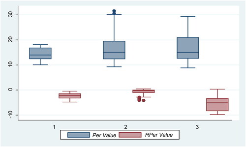
For visualisation, we present a multiple box plots (Figure 1) of Per value and Rper value with different dividend payout ratio. The shape of the cross-group distribution of Rper value in Figure 1 supports the conclusion that moderate payment of cash dividends to shareholders can increase the persistence of earnings, which also provides evidence for the implementation of a semi-mandatory cash dividend system in China. However, the cross-group distribution of Rper values does not reflect trend-significance.

Figure 1. Multiple box plots of Per value and RPer value with different dividend payout ratio (from low to the high).

Source: Authors’ calculation.

3.3.3.2. Regression results based on classification of dividends payout ratio characteristics

Table 6 provides the combined regression results based on classification of corporate dividends payout ratio: (1) In the group of ‘Iron Rooster’ firms with zero D.P.R., all the regression coefficients between earnings response coefficient, Per value and Rper value are negative, in which the regression coefficient of Per value is −1.049 and its t value is significant at the 1% level, indicating that investors have a negative response to earning persistence measueres when firms pay zero cash dividends; (2) In the corresponding high D.P.R. group, all the regression coefficients between earnings response coefficient, Per value and Rper value are positive, indicating that investors have a positive response to earning persistence measueres when firms pay high cash dividends; and (3) In the medium D.P.R. group, all the regression coefficients between earnings response coefficient, Per value and Rper value are positive, in which the regression coefficient of Rper value is 0.623 and its t value is significant at the 1% level, indicating that investors have a significant positive response to earning persistence measures of Rper value when firms pay medium cash dividends. Comprehensive (1) to (3), it shows that investors have made a correct response to the earnings persistence measure constructed in this article, especially for the medium dividends paying firms. The regression results based on the characteristics of dividends payment factors also prove the usefulness of the earnings persistence measure constructed in this article.

3.3.4. Descriptive statistics and analysis by characteristics of firm’s R.O.E

To further illustrate the effect of the R.O.E. on our Rper value of the earning persistence measure, the 872 listed firms are divided into five groups according to the size of the R.O.E. from low to high, the descriptive statistics are shown in Table 7.

Table 7. Descriptive statistics by characteristics of firms’ ROE.

ROE (from low to high)	N	Unexpected earnings response coefficient			Per value			RPer value			ROE			Dividends payout rate
		Min.	Max.	Mean	Min.	Max.	Mean	Min.	Max.	Mean	Min.	Max.	Mean	Min.	Max.	Mean
1	175	−136.25	42.85	1.58	5.55	74.37	16.43	−11.47	−1.65	−3.81	0.00	0.01	0.01	0.00	0.46	0.11
2	175	−47.32	24.48	1.31	7.30	43.46	16.35	−1.65	−0.58	−1.02	0.01	0.02	0.01	0.00	0.33	0.08
3	174	−12.76	58.69	2.19	8.15	129.89	17.49	−0.57	−0.14	−0.33	0.02	0.02	0.02	0.00	0.23	0.07
4	174	−46.07	52.63	1.18	6.37	53.15	16.34	−0.14	0.14	0.01	0.02	0.03	0.02	0.01	0.22	0.08
5	174	−20.99	37.06	2.30	6.21	59.97	19.39	0.15	0.77	0.34	0.03	0.10	0.04	0.00	0.26	0.09
Total sample	872	−136.25	58.69	1.71	5.55	129.89	17.20	−11.47	0.77	−0.96	0.00	0.10	0.02	0.00	0.46	0.08

Source: Authors’ calculation.

Table 7 indicates that: (1) The mean value of the quarterly R.O.E. for the highest group is 0.04 and 0.01 for the lowest group, while the mean value of the corresponding dividends payout ratio is 0.07–0.09 except for group 1 (which is 0.11), these statistics shows that the payment of cash dividends is not affected by the performance of the company. (2) As for the mean value of the Per value constructed by Kormendi and Lipe’s, the highest group is 19.93 and the lowest group is 16.34, besides, the statistics display upward trend, which indicate that the higher the R.O.E., the more persistence of the firm’s earnings, but its change is not gradual. (3) The mean value of the Rper reveals that, the Rper value of the high and low groups are −3.81 and 0.34, respectively, which also presents a clear and gradual upward trend, and their magnitude of change is larger. Comparing the corresponding R.O.E., the mean value of the lowest group are is 0.01 and the mean value of the highest group is 0.04, while their corresponding minimum and maximum value is 0, 0.01 and 0.03, 0.04, respectively. Obviously, with similar dividends payout rates, differences in R.O.E. determine the differences in earnings persistence, which is consistent with the findings of the theoretical analysis in section 2.3.

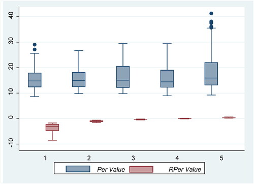
We also introduce a multiple box plots to illustrate the trend and distribution of earnings persistence with different level of R.O.E., so as to provide an intuitive insight. The box plots of the Rper value in Figure 2 display a clear and gradual upward trend, which indicate that the higher the R.O.E., the more persistence of the firm’s earnings. In addition, the divergence in trends also proves that Rper value of our model may have more explanatory power than that of Kormendi and Lipe’ model.

Figure 2. The multiple box plots of Per and RPer with different R.O.E. (from low to the high).

Source: Authors’ calculation.

3.3.5. Results of descriptive statistics and empirical regression tests and analyses by firm size (sales) characteristics²

According to Baginski et al. (1999), size factors are important determinants on earnings persistence. In order to understand China’s listed firms’ size characteristics in terms of cash dividends payout rate, R.O.E., and earnings persistence, the 872 sample are divided into five groups according to the size of total sales from low to high, the descriptive statistics and regression results of Per value, Rper value and earnings reaction coefficient for different size are show in Table 8 and Table 9, respectively.

Table 8. Descriptive statistics based on firm size characteristics (sales) classification.

Size (from low to high)	N	Earnings response coefficient			Per value			RPer value			ROE			Dividends payout rate
		Min.	Max.	Mean	Min.	Max.	Mean	Min.	Max.	Mean	Min.	Max.	Mean	Min.	Max.	Mean
1	175	−47.32	52.63	1.91	5.55	74.37	15.45	−9.98	0.59	−1.46	0.00	0.06	0.02	0.00	0.45	0.08
2	175	−46.07	53.12	2.65	6.21	53.15	16.49	−11.47	0.71	−1.16	0.00	0.08	0.02	0.00	0.46	0.09
3	174	−136.25	34.10	1.37	7.30	49.86	17.21	−10.60	0.63	−1.06	0.00	0.06	0.02	0.02	0.30	0.09
4	174	−12.59	58.69	1.98	6.37	129.89	17.91	−7.50	0.77	−0.55	0.00	0.10	0.02	0.00	0.33	0.08
5	174	−13.01	25.90	0.64	7.30	59.26	18.94	−8.29	0.69	−0.58	0.00	0.07	0.02	0.00	0.46	0.08
Total	872	−136.25	58.69	1.71	5.55	129.89	17.20	−11.47	0.77	−0.96	0.00	0.10	0.02	0.00	0.46	0.08

Source: Authors’ calculation.

Table 9. Combined regression results of Per, RPer and unexpected earnings response coefficient.

Size	N	Intercept (${\omega }_0$)	Coefficients for Per value (${\omega }_1$)	Coefficients for RPer value (${\omega }_2$)	Adj_R^2	VIF
High-sales	436	2.375* (1.69)	0.0417 (0.55)	0.710*** (2.60)	0.012	1.02
Low-sales	436	1.129* (1.87)	0.0143 (0.50)	0.157 (0.85)	−0.002	1.12
Total sample	872	1.854*** (2.63)	0.0169 (0.48)	0.448*** (2.64)	0.006	1.00

Note: t-statistics are shown in parentheses. Significance (two-tailed) at the 0.1, 0.05 and 0.01 levels are indicated by *, ** and ***, respectively. Since all of the VIF are near to 1 (less than 2), multicollinearity does not pose an issue for the analysis.

Source: Authors’ calculation.

3.3.5.1. Descriptive statistics and analysis based on the classification of firm size characteristics

Table 8 presents that: (1) The mean value of quarterly R.O.E. are all 0.02 from the smallest size of firms to the largest size of firms, indicating that there are no differences in R.O.E. among different firm size. (2) The mean value of RPer constructed in this article are −1.46, −1.16, −1.06, −0.55, −0.58, presenting an obvious trend of increasing from small to large with the size of firms, these results are consistent with Jacobsen (1988), Baginski et al. (1999), whose findings claim a significant positive correlation between firm’s size and earnings persistence. (3) The mean value and the minimum and maximum value of the Per of Kormendi and Lipe’s earnings persistence measure present that, the minimum and maximum value change with stable characteristics, stable between 5.55–7.30 and 49.86–129.89, respectively, while the mean value also shows a significant gradual change from small to large as the size of the firm increases, with Per value of 15.45, 16.49, 17.21, 17.91, and 18.94, respectively. These analysis above suggest that the Chinese regulators can set different standards of mandatory cash dividends system according to the size of firms.

3.3.5.2. Regression results and analysis based on firm size characteristics classification

Table 9 reports the combined regression results of Per value, RPer value and unexpected earnings response coefficient. (1) The regression coefficients of the earnings response coefficients with RPer value show that, the regression coefficient for high sales is 0.710 and its t-value is significant at the 1% level (two-sided), while the regression coefficient for low sales is 0.157 and its t-value is also significant, and the regression coefficient for low-sales firms is lower than that for high-sales firms, which indicates that the RPer value by this article has more explanatory power for large firms. (2) The regression coefficients of the earnings response coefficient and Per value are 0.0417 and not significant for high sales firms and 0.0143 and not significant for low sales firms. In conclusion, the classification based on the characteristics of the size further demonstrates the usefulness of the earnings persistence measures constructed in this article.

4. Research findings and policy recommendations

In response to the inadequacy of existing research on earnings persistence, we construct a more realistic earnings persistence measure-RPer value, and find that dividends payout ratio has little effect on the earnings persistence, while R.O.E. has a decisive effect on earnings persistence; besides, the earnings persistence measure developed by Lipe (1990) is a specific form of RPer value. Using the quarterly data of Chinese listed firms from 2011 to 2020, we calculate the RPer value, Per value and earnings reaction coefficient of each firm, and conduct univariate and combined regression tests on the relation between the unexpected earnings reaction coefficient of the quarterly earnings and the RPer value, as well as Per value. The results indicate that the RPer value has a stronger and significant explanatory power than that of Per value, which demonstrates the usefulness of our earnings persistence model under more realistic assumptions.

Our theoretical model and empirical results are also policy-relevant. (1) The RPer value of our model measuring earnings persistence reveals that profitability (R.O.E.) plays a key role in the impact of earnings persistence, which implies that even the ‘Iron Rooster’ firms that do not pay dividends but reinvest all its profits may have low earnings persistence if its investment efficiency is low; on the contrary, even if the firm distributes all its profits to its shareholders, the measure of earnings persistence will still be large if the investment efficiency is high. Therefore, our theoretical results can provide strong support the semi-mandatory cash dividends system implemented in China. (2) The empirical results of the classification based on dividend payout rate, R.O.E., and firm size indicate that dividend payout rate has little impact on the persistence of earnings; however, firm size is positively correlated with the persistence of earnings, so the Chinese regulators can also implement different mandatory cash dividend systems by firm size; further, as industries with high R.O.E. have the highest RPer value for the persistence measure of earnings, the regulators could also implement different mandatory cash dividends regimes based on industry classification.

Disclosure statement

No potential conflict of interest was reported by the authors.

Additional information

Funding

This work was supported by the National Natural Science Foundation of China (No. 72002068), National Social Science Foundation of China (No. 19BJY038), Central Universities Basic Research Funds for Humanities and Social Sciences Projects (No. 2020CDJSK02PT03) and Chongqing Federation of Social Sciences (No. 2019WT40).

Notes

1 Model selection steps:

a) Getting the observed sample time-series [X _{j, t}: Earnings Per Share].

b) Plotting the data to observe whether the series is stationary; for the non-stationary series, perform d-order differencing, and then according to the result of the ADF-test, get the order of differenced d.

c) Calculating the Autocorrelation Coefficient (A.C.F.) and the Partial Autocorrelation Coefficient (P.A.C.F.) respectively, getting the potential range of order p and q by observing the autocorrelation and partial autocorrelation plots; then taking the A.I.C. and S.I.C. criteria (the combination of p and q that minimizes the A.I.C. or S.I.C. is selected) to determine the parameter p and q of the optimal A.R.I.M.A. model.

2 Our research also includes the descriptive statistics and empirical test based on industry classifications. However, subject to the guidelines for article length, we do not present the results. If interested, we are glad to share.

References

- Adhikari, B. K., & Agrawal, A. (2018). Peer influence on payout policies. Journal of Corporate Finance, 48, 615–637. https://doi.org/10.1016/j.jcorpfin.2017.12.010
- Baginski, S. P., Lorek, K. S., Willinger, G. L., & Branson, B. C. (1999). The relationship between economic characteristics and alternative annual earnings persistence measures. The Accounting Review, 74(1), 105–120. https://doi.org/10.2308/accr.1999.74.1.105
- Ball, R., & Brown, P. (1968). An empirical evaluation of accounting income numbers. Journal of Accounting Research, 6(2), 159–178. https://doi.org/10.2307/2490232
- Beaver, W. H., Lambert, R. A., & Ryan, S. G. (1987). The information content of security prices: A second look. Journal of Accounting and Economics, 9(2), 139–157. https://doi.org/10.1016/0165-4101(87)90003-6
- Bernard, V. L. (1994). Accounting based valuation methods, determinants of market-to-book rations, and implications for financial analysis [Working paper]. University of Michigan.
- Bernard, V. L., Merton, R. C., & Palepu, K. G. (1995). Mark-to-Market accounting for banks and thrifts: lessons from the danish experience. Journal of Accounting Research, 33, 1–32. https://doi.org/10.2307/2491290
- Blaylock, B., Shevlin, T., & Wilson, R. J. (2012). Tax avoidance, large positive temporary book-tax differences, and earnings persistence. The Accounting Review, 87(1), 91–120. https://doi.org/10.2308/accr-10158
- Call, A. C., Hewitt, M., Shevlin, T., & Yohn, T. L. (2016). Firm-specific estimates of differential persistence and their incremental usefulness for forecasting and valuation. The Accounting Review, 91(3), 811–833. https://doi.org/10.2308/accr-51233
- Chang, K., Kang, E., & Li, Y. (2016). Effect of institutional ownership on dividends: An agency-theory-based analysis. Journal of Business Research, 69(7), 2551–2559. https://doi.org/10.1016/j.jbusres.2015.10.088
- DeAngelo, H., DeAngelo, L., & Skinner, D. J. (2000). Special dividends and the evolution of dividend signaling. Journal of Financial Economics, 57(3), 309–354. https://doi.org/10.1016/S0304-405X(00)00060-X
- Dechow, P. M., Ge, W., & Schrand, C. (2010). Understanding earnings quality: A review of the proxies, their determinants and their consequences. Journal of Accounting and Economics, 50(2-3), 344–401. https://doi.org/10.1016/j.jacceco.2010.09.001
- Denes, M. R., Karpoff, J. M., & McWilliams, V. B. (2017). Thirty years of shareholder activism: A survey of empirical research. Journal of Corporate Finance, 44, 405–424. https://doi.org/10.1016/j.jcorpfin.2016.03.005
- Eesterbrook, F. H. (1984). Two agency-cost explanations of dividends. American Economic Review, 74(4), 650–659. https://doi.org/10.2307/1805130
- Flavin, M. A. (1981). The adjustment of consumption to changing expectation about future income. Journal of Political Economy, 89(5), 974–1008. https://doi.org/10.1086/261016
- Frankel, R., & Litov, L. (2009). Earnings persistence. Journal of Accounting and Economics, 47(1-2), 182–190. https://doi.org/10.1016/j.jacceco.2008.11.008
- Gong, Y., Yan, Y., & Yang, N. (2021). Does internal control quality improve earnings persistence? Evidence from China’s a-share market. Finance Research Letters, 42, 101890. https://doi.org/10.1016/j.frl.2020.101890
- Grennan, J. (2019). Dividend payments as a response to peer influence. Journal of Financial Economics, 131(3), 549–570. https://doi.org/10.1016/j.jfineco.2018.01.012
- Jacobsen, R. (1988). The persistence of abnormal returns. Strategic Management Journal, 9(5), 415–430. https://doi.org/10.1002/smj.4250090503
- Jenson, M. C. (1986). Agency costs of free cash flow, corporate finance, and takeovers. The American Economic Review, 76(2), 323–329. https://doi.org/10.2139/ssrn.99580
- Jiraporn, P., Kim, J. C., & Kim, Y. S. (2011). Dividend payouts and corporate governance quality: An empirical investigation. Financial Review, 46(2), 251–279. https://doi.org/10.1111/j.1540-6288.2011.00299.x
- Klein, A., & Zur, E. (2009). Entrepreneurial shareholder activism: Hedge funds and other private investors. The Journal of Finance, 64(1), 187–229. https://doi.org/10.1111/j.1540-6261.2008.01432.x
- Kormendi, R., & Lipe, R. (1987). Earnings innovations, earnings persistence, and stock returns. The Journal of Business, 60(3), 323–345. https://doi.org/10.1086/296400
- Harakeh, M. (2020). Dividend policy and corporate investment under information shocks. Journal of International Financial Markets, Institutions & Money, 65, 101184. https://doi.org/10.1016/j.intfin.2020.101184
- La Porta, R., Lopez, D. F., Shleifer, A., & Vishny, R. W. (2000). Agency problems and dividend policies around the world. The Journal of Finance, 55(1), 1–33. https://doi.org/10.1111/0022-1082.00199
- Lipe, R. C. (1990). The relation between stock returns and accounting earnings given alternative information. The Accounting Review, 65(1), 49–71.
- Mahdzan, N. S., Zainudin, R., & Shahri, N. K. (2016). Interindustry dividend policy determinants in the context of an emerging market. Economic Research-Ekonomska Istraživanja, 29(1), 250–262. https://doi.org/10.1080/1331677X.2016.1169704
- McCahery, J., Sautner, A., & Starks, L. T. (2016). Behind the scenes: The corporate governance preferences of institutional investors. The Journal of Finance, 71(6), 2905–2932. https://doi.org/10.1111/jofi.12393
- Miller, M. H., & Modigliani, F. (1961). Dividend policy, growth and valuation of shares. Journal of Business, 34, 411–435. https://doi.org/10.1086/29444
- Modigliani, F., & Miller, M. H. (1958). The cost of capital, corporation finance and the theory of investment. American Economic Review, 48(3), 261–297. https://doi.org/10.1080/00346765900000019
- Mueller, D. C. (1977). The persistence of profits above the norm. Economica, 44(176), 369–380. https://doi.org/10.2307/2553570
- Ohlson, J. A. (1995). Earnings, book value, and dividends in equity valuation. Contemporary Accounting Research, 11(2), 661–687. https://doi.org/10.1111/j.1911-3846.1995.tb00461.x
- Penman, S. H. (1991). An evaluation of accounting rate of return. Journal of Accounting, Auditing & Finance, 6(2), 233–255. https://doi.org/10.1177/0148558X9100600204
- Rozeff, M. S. (1982). Growth, beta and agency costs as determinants of dividend payout ratios. Journal of Financial Research, 5(3), 249–259. https://doi.org/10.1111/j.1475-6803.1982.tb00299.x