A study of household income inequality in China: perspective of educational homogeneity marriage

Abstract

Based on the data from the 2006 to 2017 Chinese Social Survey (C.S.S.), we measured the extent of inequality between the total household income and the average household income in China. We conclude that the Gini coefficient of total household income fluctuates between 0.47 and 0.52. The Gini coefficient of household per capita income fluctuates between 0.5 and 0.54, indicating a significant degree of household income inequality in China. We use the kernel density method to obtain the distribution of household income and find that the overall income level of society has increased. Still, the degree of household income inequality has been growing. From the perspective of educational homogeneity marriage, we use the income distribution table to analyse the internal structure of the total household income and draw the following conclusions. High-income households account for most of the whole social gain, and an increase in household income disparities has accompanied the increase in the household size. In addition, the distribution of total household income in China differs significantly in the household head's educational attainment. A relatively small number of households with a high degree of educational attainment account for a relatively large share of income, and households with a combination of high–high and high–low educational attainment have gradually increased. The proportion of social income has continued to rise.

Keywords:

• household
• educational homogeneity marriage
• household income gap
• income distribution table

SUBJECT CLASSIFICATION CODES:

• D10; D31; D13

1. Introduction

For 40 years since the reform and opening-up, China's G.D.P. has continued to climb. In 2015, China's per capita G.D.P. reached US$8,000. Economic growth has slowed down in the previous decade, but people's living standards have improved substantially. But at the same time, the income gap in China is getting more and more severe. In the early 1980s, the Chinese social Gini coefficient remained at around 0.2. Since 2000, the Gini coefficient has continued to exceed 0.4. The official Gini coefficient in 2018 was 0.474, far exceeding the international warning line of 0.4. The Gini coefficient of per capita household income and total household income fluctuates around 0.5. The Gini coefficient of household net wealth once exceeded 0.5, and the hidden income of high-income people makes this data most likely to be underestimated.

In the ‘Report on Household Income Inequality in China’ published by Southwestern University of Finance and Economics in 2012, according to the China Household Finance Survey (C.H.F.S.) data, the Gini coefficient of household income in China was calculated to be 0.61 in 2010, the Gini coefficient within urban households was 0.56, the Gini coefficient within rural households was 0.60 (China Household Finance Survey and Research Center, 2012).

The new family economics believes that the family is a broad economic behaviour subject. The culture of ‘family deeply influences Chinese residents’, and purchase expenditures or consumer service activities are all based on the family (Xinjian & Jinchang, 2005). Income will also be managed and distributed by the family. The total family income determines the quality of life of all family members, while the income of a married family is mainly composed of the wages of both spouses. Educational attainment is the main factor affecting income in the human capital market. Therefore, excluding the effect of wealth income, the matching of the educational attainment of the couple and the education level of their children determines the family income level. It is of tremendous research significance to focus on family income inequality from homogenous educational marriage.

The other parts of this article are as follows: Section 2 gives a literature review; Section 3 presents the theoretical derivation and hypothesis of the effect of education on household income inequality in the family structure; Section 4 introduces data sources and measures total and per capita income inequality of Chinese households; Section 5 gives the structural distribution of household income inequality, and discusses and explains it; Section 6 is the research summary and recommendations.

2. Literature review

2.1. Influencing factors of income inequality

Income inequality has different manifestations in different economic forms (Han, 2010), the influencing factors are also diverse. According to previous studies, the main factors affecting the individual income gap include gender (Bertrand et al., 2010; Gordon & Dew-Becker, 2008). Education level and skills (Baum-Snow & Pavan, 2013; Duranton & Puga, 2004), region (Acemoglu, 2003; Moretti, 2004), race (Lang & Lehmann, 2011), technological change (Antonelli & Gehringer, 2017; Mon & Kakinaka, 2020), etc. The influencing factors that affect the family income gap mainly include location, single parent, women's participation in the labour market (Esping-Andersen, 2007), family marriage structure, husband and wife education level, political capital (Cao & Qian, 2021), etc. In addition, education, as the core factor that determines the level of human capital, determines the distribution of income among individuals and families to a certain extent. Amaa (2020) analysed the impact of human capital (education and experience) and social factors (gender, marital status, spatial conditions and occupation) on Bangladesh based on 9943 samples of the Household Income and Expenditure Survey (H.I.E.S.) through O.L.S. and quantile regression. Xiwei (2011) took the family as the research unit and found that the region, the education level of the head of the household, and the political status significantly impact household income and wealth inequality.

In the research on the impact of the household income gap between urban and rural areas, scholars found that the correlation between rural income inequality and household income inequality is very weak, and the proportion of high-income households in urban areas is higher than that in rural areas (Haigang, 2005b; Zexia et al., 2011). In addition, as the link between individuals and families, the matching pattern of marriage directly impacts the distribution of family income. However, the impact of the educational structure of marriage on the family income gap is still inconclusive. Kremer (1997) used a dynamic model of marriage-matching to find the proportion of educational homogeneity marriages in the U.S. during the 20th century. Still, it did not change the income gap in the U.S. Subsequently, Breen and Salazar (2011) showed that educational homogeneity marriage only changed the income inequality within the group and had no significant effect on the overall income gap. The ‘strong alliance’ will further aggravate the family income gap with the positive marriage match. Greenwood et al. (2014) believe that Positive Assortative Matching (P.A.M.) is a significant factor leading to income inequality. The effect of educational homogeneity on the income gap will have different results for different research objects, with inter-country differences (Eika et al., 2019). Chinese scholars have concluded that the educational matching degree of marriage in China is increasing, further widening the income gap between Chinese families (Liqun et al., 2015; Qiuchuan, 2018).

2.2. Measurement indicators of income inequality

The indicators commonly used to measure income inequality are the Gini index, Lorenz curve, Theil index, and income distribution table. The Gini coefficient is the most widely used index to measure income inequality. Considering the representativeness of the sample, the advantage of the Gini coefficient lies in the decomposability between the income gaps of different sub-items. The advantage of the Lorenz curve is that it can group incomes and thus identify between which groups income disparities occur. The Theil index can decompose the national income gap into inter-regional and intra-regional. The income distribution table was pioneered by Piketty (2017), which analyses the internal structure of income inequality by dividing the sample group and calculating the ratio of the total social income.

There is also extensive literature on the measurement of household income inequality. Grow and Van Bavel (2020) developed a method to decompose the structure of income inequality by income elements. This approach quantifies changes in the association between revenue sources. It can also analyse the impact of changes in marginal distribution on changes in household income distribution. Discrete distribution is only suitable for numerical data, but it can cover more survey information; Continuous distribution can be subdivided into parametric estimation and semi-parametric estimation, but the premise of parametric analysis is to determine the specific function form and then estimate the parameters through survey data to obtain the income distribution function (Chotikapanich et al., 2007; Haigang & Kaiguo, 2006; McDonald & Jensen,1979; Schmittlein, 1983; Zhijun, 2012). The study of Jinghui and Jianbao (2010) found that the per capita income of households in China follows a mixed distribution, including Pareto distribution, normal distribution, an exponential distribution.

2.3. Measurement of household income inequality

The measure of income inequality is related to the unit of measurement. The calculated data will be different when we measure the same income inequality separately based on individuals, families, and households (Atkinson & Bourguignon, 2000). New family economics considers the family the smallest unit of economic activity. China's unique national situation is deeply influenced by traditional family culture. Households make most purchases, and most statistics are collected from households or families. Therefore, it is necessary to take household income distribution as the research object. There are many measurement results of the Chinese household income gap.

Based on Chinese Household Income Project (C.H.I.P.) data, Shi (2015) measured that the Gini coefficient of the household income gap in China was 0.409 in 1995. The Gini coefficient of household income measured by Haigang (2005a) through China Health and Nutrition Survey (C.H.N.S.) data is similar to that of Li Shi. In 1989, 1991 and 1993, the Gini coefficients of household income in China were 0.427, 0.389 and 0.47, respectively. It was evident that the income gap between Chinese households has changed since marketisation. Using C.H.F.S. data, Southwest University of Finance and Economics (S.W.U.F.E.) measured that the Gini coefficient of household income in China exceeded 0.6 in 2010. Therefore, some scholars questioned that this data seriously overestimated the extent of income inequality of Chinese households. Based on household survey data, Xie and Zhou (2014) obtained that the Gini coefficient of household income in China was about 0.54 in 2010–2012. After considering the implicit income of households, Qiongzhi and Qin (2015) estimated that the Gini coefficients of Chinese households were 0.4987 and 0.5316 in 2007 and 2011, respectively. This figure is also smaller than the Gini coefficient of Chinese household income measured by the Southwestern University of Finance and Economics. Jinbao and Li (2013) used household consumer finance survey data from 24 cities to discuss the distribution of household income in Chinese cities. The conclusion is that the Gini coefficient of household income of Chinese urban residents is between 0.36267 and 0.38216.

There is much literature on the measurement of household income inequality in China. Most scholars focus their research on the influencing factors of the household income gap and the measure of household inequality. There is a lack of research on the long-term dynamics of the household income gap in China. The discussion of internal structural characteristics, especially the role of marriage structure in family income inequality, is ignored. This article uses the data of the Chinese Social Survey (C.S.S.) from 2006 to 2017 to measure the inequality of total household income and average household income in China. Based on the structural analysis method, discuss the internal system of structural inequality in China and analyse the internal structure of household income inequality in China from homogeneous educational marriage.

3. Estimation techniques

In the theory of this article, only the income generated by human capital is regarded as the only source of income; that is, the total household income is equal to the sum of the salary income of each family member. For research convenience, we assume that a family has only three family members, namely the husband, wife and children. It is believed that each family has only one child. The child will need education in early childhood, which will need education costs. And in adulthood, the child earns income through work. Therefore, we set up an intergenerational overlap model with two periods, including childhood and adulthood. According to the enrolment age of Chinese students, the age for a student to complete higher education is 22 years old. The period below 22 years old is called childhood, and the period above 22 years old is called adulthood. Individuals have different educational choices. For the convenience of research, we simplified the educational attainment to high and low: the type with higher education is denoted as $H,$ and the type of no higher education is represented $D.$ To simplify the model, we will no longer discuss the interference of family background on an individual's marriage selection and only consider the probability of one's educational attainment for spouse selection. The probability that youth with high educational attainment chooses a spouse with high educational attainment is ${\alpha }_H,$ then the probability of choosing a spouse with low educational attainment is $1-{\alpha }_H.$ The likelihood youth with low educational attainment choosing a spouse with high educational attainment is ${\alpha }_D,$ and the probability of choosing a spouse with low educational attainment is $1-{\alpha }_D.$ Assume that the average annual salary of a social member with high educational attainment is $W_H,$ and the average yearly salary of a social member with low educational attainment is $W_D.$

Assume that the probability of a child born from a family with a combination of high–high educational attainment to become a social member with high educational attainment is ${\beta }_2,$ the likelihood of a child born from a family with a variety of high–low educational attainment to become a social member with high educational attainment is ${\beta }_1.$ The probability of a child born from a family with a combination of low–low educational attainment is to become a social member with high educational attainment is ${\beta }_0.$ At the same time, the education of young children requires education costs. Since China has implemented a nine-year compulsory education policy, it is assumed that there is no cost for low-degree education, and the annual cost per person for high-degree education is recorded as $C.$ We propose the following three hypotheses based on the above comment – hypothesis 1. We hypothesise ${\alpha }_H>{\alpha }_D.$ According to the matching theory of homogeneity marriage, social members with high educational attainment are more likely to choose youth with high educational attainment as their spouses – hypothesis 2. We hypothesise $W_H>W_D.$ From the perspective of human capital, the average salary of social members with high educational attainment is more likely to be higher than social members with low educational attainment without considering the physical capital – hypothesis 3. We hypothesise ${\beta }_2>{\beta }_1>{\beta }_0.$ The intuitive meaning is that it is easier for families with high–high educational attainment to cultivate educational attainment social members.

First of all, families with higher educational attainment have higher incomes and can afford higher educational expenditure, training costs, tutors and other expenditure, etc.; Secondly, families with higher educational attainment will pay more attention to the education of their children and be stricter with the education of their children, which are the independent choices of the families.

In this model, if the head of the household $\mathrm{i}$ is a social member with high educational attainment and the child is in childhood, the expected revenue of the household is as follows. (1) $$E{Y}_{iH}^1=W_H+{\alpha }_H{W}_H+\left(1-{\alpha }_H\right)W_D-\left[{\alpha }_H{\beta }_2+\left(1-{\alpha }_H\right){\beta }_1\right]\cdot C$$(1) if the head of the household $\mathrm{i}$ is a social member with low educational attainment and the child is in childhood, the expected revenue of the household is as follows. (2) $$E{Y}_{\mathrm{i}D}^1=W_D+{\alpha }_D{W}_H+(1-{\alpha }_D)W_D-\left[{\alpha }_D{\beta }_1+\left(1-{\alpha }_D\right){\beta }_0\right]\cdot C$$(2)

According to the hypothesis, the expected revenue of the family with high educational attainment is greater than or equal to the family with low educational attainment. And we have to consider the education threshold. When the income is higher than the cost of education for the child, the child will have the opportunity to receive high education. Therefore,$E{Y}_{\mathrm{i}D}^1\ge C$ is needed, and after calculating according to Equation (2)(2) $$E{Y}_{\mathrm{i}D}^1=W_D+{\alpha }_D{W}_H+(1-{\alpha }_D)W_D-\left[{\alpha }_D{\beta }_1+\left(1-{\alpha }_D\right){\beta }_0\right]\cdot C$$(2) , we get: (3) $$C\le \frac{W_D+{\alpha }_D{W}_H+(1-{\alpha }_D)W_D}{{\alpha }_D{\beta }_1+(1-{\alpha }_D){\beta }_0}$$(3)

When Equation (3)(3) $$C\le \frac{W_D+{\alpha }_D{W}_H+(1-{\alpha }_D)W_D}{{\alpha }_D{\beta }_1+(1-{\alpha }_D){\beta }_0}$$(3) is established, the value $C$ is the threshold value of higher education. Only when the family income is higher than the education threshold can children have the opportunity to receive higher education and bring increased revenue to the family after they become adults.$W_H$ and $W_D$ are exogenous variables, so the size of the education threshold is related to the size of ${\alpha }_D,$ ${\beta }_1$ and ${\beta }_0.$ With a certain income level, the higher the probability of a child from an ordinary family receiving higher education, the higher the education threshold. This is also consistent with reality. When there are specific educational resources, the more people can access higher education, the higher the education threshold, the increasing education threshold by the involution of education cannot even be solved by raising income levels. It can increase the rate of higher education only by increasing educational resources.

Education can bring high income, but the prerequisite for increased revenue is obtaining high educational attainment. The household burden is heavier during children's childhood, and then we analyse the total household income level of the children in adulthood. During the children's maturity, there are three labourers in the family, and the sum of the income of each family member is the total family income. It is the same as the hypothesis of the children's childhood, but the adult children no longer need education costs, and they will bring different incomes due to differences in educational attainment.

In this model, if the head of the household $\mathrm{i}$ is a social member with high educational attainment and the child is in adulthood, the expected revenue of the household is as follows. (4) $$E_{iH}^2=W_H+{\alpha }_H{W}_H+\left(1-{\alpha }_H\right)W_D+\left[{\alpha }_H{\beta }_2+\left(1-{\alpha }_H\right){\beta }_1\right]W_H+\left[1-{\alpha }_H{\beta }_1+\left({\alpha }_H-1\right){\beta }_2\right]W_D$$(4) if the head of the household $\mathrm{i}$ is a social member with low educational attainment and the child is in adulthood, the expected revenue of the household is as follows. (5) $$E_{iD}^2=W_D+{\alpha }_D{W}_H+\left(1-{\alpha }_D\right)W_D+\left[{\alpha }_D{\beta }_1+(1-{\alpha }_D){\beta }_0\right]W_H+\left[1-{\alpha }_D{\beta }_1+\left({\alpha }_D-1\right){\beta }_0\right]W_D$$(5)

From the perspective of the human capital of education, the total household income gap is simplified to the difference between the expected revenue of the household with high educational attainment and low educational attainment, that is, $E_{iH}^1-E_{iD}^1$ and $E_{iH}^2-E_{iD}^2.$$W_H$ and $W_D$ are exogenous variables. The total household income gap is related to the size of ${\alpha }_H$、${\alpha }_D$、${\beta }_2$、${\beta }_1$、are ${\beta }_0.$${\alpha }_H$ and ${\alpha }_D$ determine whether a social member will choose educational homogeneity marriage. According to the research results of many scholars, ${\alpha }_H>{\alpha }_D$ that is, young people with high educational attainment are more likely to form a couple with young people with high educational attainment, which will naturally widen the income gap.

From this, we can draw two inferences: First, the educational attainment of an individual will affect the educational attainment of spouses and children, and the increase in the proportion of educational homogeneity marriages may widen the household income gap; second, an increase in the rate of higher education will increase the cost of education. Low-income people will fall into a poverty trap, and the probability of children from low-income families will decline. The vicious circle will further aggravate the household income gap.

4. Analysis of household income inequality in China

4.1. Data source

The data used in this article mainly comes from the C.S.S. from 2006 to 2017. The survey is a biennial longitudinal survey using probability sampling for household interviews. To demonstrate the dynamic changes in household income inequality in China, this article uses 6 periods of data from 2006 to 2017 (2006, 2008, 2011, 2013, 2015, 2017) as the research basis. We eliminated invalid data and missing data and finally got, respectively: 6789, 6777, 6847, 9502, 9644, 9554 valid samples.

4.2. Descriptive statistical analysis

Below we give different descriptive statistical results of the total household income and per capita household income for the six years from 2006 to 2017 and analyse the current status of household income inequality in China for this decade.

From the statistical result of total household income and average household income in Table 1, we find that the average household income and average household income per capita in China have increased from 2006 to 2017. It should be noted that the standard deviation reached its maximum in 2011 and 2013, which can roughly infer that the household income gap is relatively high in these two years. The skewness and peak value of the total household income and per capita household income are more significant than zero in the six years, indicating that total revenue and per capita accurate income distribution are tailing and right-skewed distributions. The skewness and peak value of the total household income and per capita household income in all six years are higher than zero, indicating that the distribution of total revenue and per capita income are tailing and right-skewed distributions patterns.

Table 1. Total and per capita household income in China.

Year	Total household income				per capita household income
	Mean	Standard Deviation	Skewness	Peak	Mean	Standard Deviation	Skewness	Peak
2006	19399	44040	47.1	3104.1	6429	20259	59.77	4357.7
2008	28662	38395	10.39	225.3	8204	11413	8.35	149.8
2011	55897	161164	41.45	2344.4	19563	38893	27.75	1201.6
2013	59708	162318	40.51	2202.2	15647	49212	40.67	2004
2015	64023	100813	16.04	481.1	16733	28510	19.11	681.28
2017	66252	135070	44.26	3094.5	17319	26516	13.11	368.2

Source: CSS survey data from 2006 to 2017.

4.3. Measurement of inequality index

In studying income inequality, the most used method is the centralised measurement method. This article reports the index to measure the degree of household inequality, and the Gini coefficient and Theil index are selected. Table 2 shows the inequality measurement results of total household income and per capita household income in 2006, 2008, 2011, 2013, 2015 and 2017.

Table 2. Measurement results of inequality index.

Year	Total household income		per capita household income
	Gini coefficient	Theil index	Gini coefficient	Theil index
2006	0.5048	0.5459	0.5355	0.6582
2008	0.4777	0.4429	0.5048	0.492
2011	0.5192	0.6618	0.5396	0.6561
2013	0.5033	0.6113	0.527	0.6843
2015	0.4955	0.4975	0.5197	0.5441
2017	0.5101	0.5388	0.5301	0.5418

Note:

^a Data source: CSS survey data from 2006 to 2017.

^b Theil index is a common form of the generalised entropy index. When the parameter is equal to 1, the generalised entropy index is similar to the Theil index. In the calculation results of the inequality index in the above table, the parameter of the Theil index is selected as 0.

In terms of the Gini coefficient, the Gini coefficients of the total household income in these six survey years were 0.5048, 0.4777, 0.5192, 0.5033, 0.4955, 0.5101, respectively, and the Gini coefficients of per capita household income were 0.5355, 0.5048, 0.5396, 0.527, 0.5197, 0.5301, respectively. Generally speaking, the Gini coefficient of household income in China is relatively high, fluctuating around 0.5, indicating that household income inequality in China is relatively greater and higher than that of individual income. According to the National Bureau of Statistics, the income Gini coefficients in 2006, 2008, 2011, 2013, 2015 and 2017 were 0.487, 0.491, 0.477, 0.473 and 0.467, respectively. This is because high-income individuals are more likely to form families with high-income individuals, and the children of high-income parents are more likely to be high-income groups. The same goes for low-income families, so household income inequality is higher. The Theil index also reflects the same problem.

Figure 1 shows the dynamic trend of the Gini coefficient of total household income and per capita household income in China from 2006 to 2017. It can be seen from Figure 1 that the inequality of per capita household income is higher than that of total household income, which is related to the composition of Chinese households. Families with higher incomes also have relatively higher social status and educational attainment and are m

Figure 1. Gini coefficient of household income in China from 2006 to 2017.

Source: CSS survey data from 2006 to 2017.

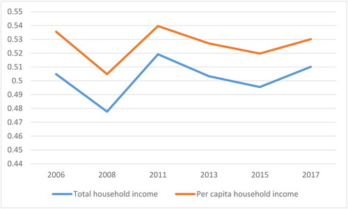
ore willing to have one child. On the other hand, the lower-income group tends to have more children and more fortune, with more population and labour force. The Gini coefficient was maintained between 0.45 and 0.55 as measured by C.S.S. data from 2006 to 2017. In terms of trends, household income inequality reached the highest in 2013, especially the Gini coefficient of total household income was as high as 0.6113. Since 2013, the Gini coefficient has declined year by year and has rebounded slightly in 2017. China raised personal income tax in 2006, 2008 and 2011, respectively, and the threshold was increased from total household income was as high as 0.6113. Since 2013, the Gini coefficient has declined yearly by total household income, and per capita, revenue declined after 2013.

4.4. Analysis of adaptive kernel density estimation

The kernel density method is a non-parametric estimation, which refers to the estimation of an unknown density function when the elemental distribution of the function data is not precise. According to the results of the descriptive statistical analysis of the six annual data given in Table 1, we can see that the peak value and skewness of the household income data are more significant than 0, which is a precise long-tailed skew-right distribution. Next, the R software is applied to simulate the peak and peak maps of the adaptive kernel density estimation of urban household total income and per capita income in the six survey years of 2006, 2008, 2011, 2013, 2015 and 2017. As shown in Figures 2 and 3.

Figure 2. Estimation of adaptive Kernel density of total household income.

Source: CSS survey data from 2006 to 2017.

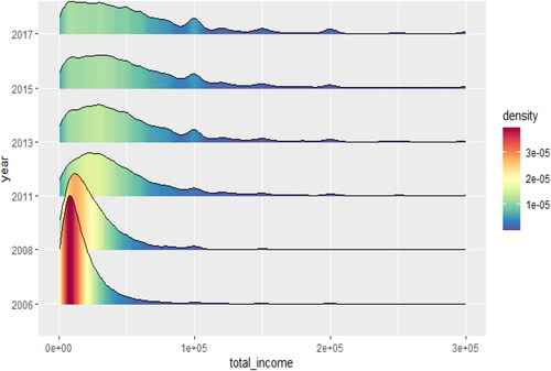
Figure 3. Estimation of adaptive Kernel density of per capita household income.

Source: CSS survey data from 2006 to 2017.

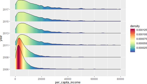
From Figures 2 to 3, the distribution of total household income and per capita household income generally shifts to the right as time goes by. The tail thickens, the length gradually increases, and the left side becomes thinner. This shows that from 2006 to 2017, the proportion of high-income households has increased, the proportion of low-income households has decreased, the overall income level of the society has increased, and residents lived more affluently. This is an inevitable result of rapid economic development. However, the kernel density map shows an increasingly flattening trend. This indicates that the total household income gap and the per capita income gap are gradually expanding, and the degree of household income inequality in China is increasing. In comparison, the kernel density peak chart of per capita household income is flatter than that of total household income. The tail is more extended, indicating that the income gap calculated by per capita household income is more significant than the actual household income gap.

5. Structural distribution of household income inequality in China

5.1. Different income quantiles

This article divides the household sample by deciles for each year based on Piketty's percentile structure analysis method to analyse the internal structure of household income inequality. We decile the number of household samples each year. We calculate the percentage of total household income in the top 10% decile of total revenue, the middle 40% decile and the bottom 50% decile, and finally, we get Figure 4.

Figure 4. Distribution of total household income in China from 2006 to 2017.

Source: CSS survey data from 2006 to 2017.

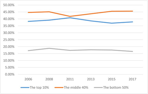
From Figure 4, from 2006 to 2017, the top 10% of households with the highest income in China received more than 35% of the total income of the entire sample, and it even reached 40% in 2011. It can be said that the top 10% of households have nearly half of the economic income of the entire sample. The middle 40% of households received 40–45% of the total household income of the whole sample, which reached 45.61% in 2017. The income ratio of the middle 40% of households is relatively stable and can represent the economic status of ordinary households. Contrary to the income of the top 10% of households, the gain of the bottom 50% of households in China is only 15–20% of the total household income of the whole sample. Over time, this proportion has decreased from 17.12% in 2006 to 16.54% in 2017. In terms of overall trends, the middle 40% of households occupy the highest income of the whole sample, followed by the top 10% of households. The gain of the top 10% of households is similar to that of the middle 40% of households and slightly lower than the median 40% of households, even reaching the same proportion in 2011. The top 10% of households account for most of the total social income, and the general trend of society is towards class consolidation.

The article classifies households with different characteristics from the perspective of household size, educational attainment of the head of family and differences in couples' education, and then analyses the internal structure of household income inequality.

5.2. Household size

Household size refers to the number of household members living together and sharing income and expenditure. According to the household size 1–15 span in the C.S.S. data, we grouped them by the number of household members. The categories are one to two family members, three family members, four family members, five to seven family members and more than seven family members. The family size of the 4-2-1 fully allocation family is 7. Figure 5 shows the distribution of the number of households of different sizes in China. Figure 6 shows the difference in scale of household income inequality in China.

Figure 5. Distribution of the number of households of different sizes in China.

Source: CSS survey data from 2006 to 2017.

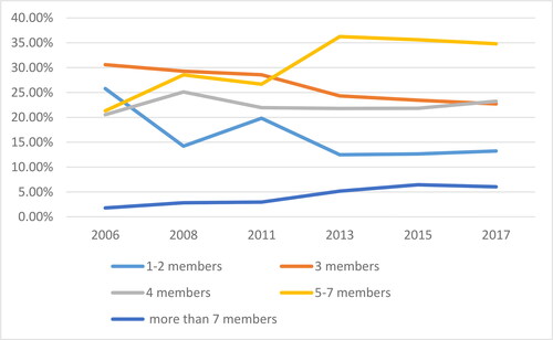
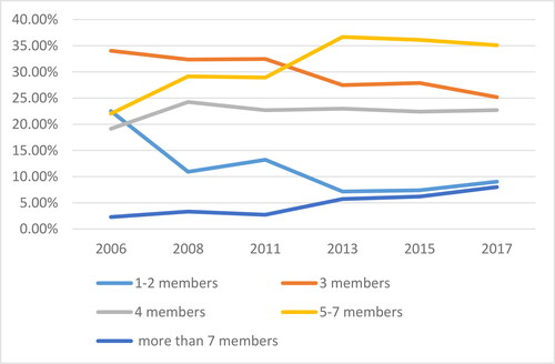
Figure 6. Distribution of total household income inequality in China: differences in household size.

Source: CSS survey data from 2006 to 2017.

From Figure 5, the size of five to seven households has gradually become the mainstream, rising from 21.31% in 2006 to 34.79% in 2017. The proportion of household size above 7 is also steadily increasing, reaching 6.03% by 2017. The ratio of households composed of one to two members and the balance of families composed of three members has decreased, especially for small-scale homes from 25.78% in 2006 to 13.23% in 2017. This shows that the size of Chinese families is getting bigger and bigger, and the fact that parents live with their adult children to help raise young children dominates society.

Figure 6 shows the household size difference in the distribution of household income inequality in China. The group with the highest total household income from 2006 to 2011 was the three-member household size group, which reached 34.04% of the total revenue in 2006. From 2013 to 2017, the highest total household income was the five to seven member household size group. Although the total income of a seven-person household has always been at the lowest proportion, this value has increased year by year. By 2017, the ratio of total household income from small to large households was 9.08:25.18:22.7:35.08:8. Compared with Figure 5, there is some overlap between the trend of the total income of households in different sizes and changes in household size. When there are more family members, there are more labourers. The household income proportion ratio should increase, but the data shows that real income has not risen. The comparison between Figures 5 and 6 shows that the expansion of household size has not increased the level of total household income. The development of household size did not reduce the household income gap. Combined with the Gini coefficient of household income, the household income gap also widened when the proportion of large-scale households increased.

On the other hand, with the increase in life expectancy and decreased fertility, China is undergoing an unprecedented demographic transformation. The proportion of the population aged 65 and over rose from 4.15% in 1949 to 12.63%. However, the social pension system started late and is not perfect enough, and families must bear part of the pension burden. The fundamental reason for the expansion of household size is to cope with the increasing cost of living and reduce the marginal expenditure of life. Therefore, the development of household size manifests the deepening of income inequality.

5.3. Educational attainment

We continue to discuss the educational factors in the family structure. Based on fully considering the household size, this article divides the sample into three groups according to the educational attainment of the head of the household. The three educational attainment groups are the low-educated, medium-educated, and high-educated groups. The low-educated group refers to household heads who have only received nine years of compulsory education or have not completed compulsory education. The educational attainment includes no education, private school, literacy class, primary school and junior high school. The medium-educated group, educational attainment includes vocational high school, ordinary high school, junior college and technical school. The high-educated group refers to household heads who have experienced higher education, and their educational attainment includes college (adult higher education), college (regular higher education), undergraduate (adult higher education), undergraduate (traditional higher education), postgraduate and above. Figure 7 shows the proportions of household heads with different educational attainment, and Figure 8 shows the difference in household income inequality education level.

Figure 7. Proportion of household heads with different educational attainment.

Source: CSS survey data from 2006 to 2017.

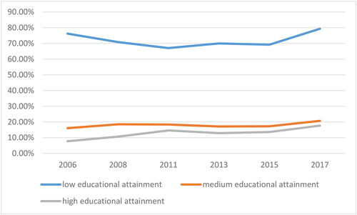
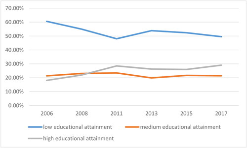
Figure 8. Inequality distribution of total household income in China: differences in the educational attainment of household heads.

Source: CSS survey data from 2006 to 2017.

In Figure 7, households with standard educational attainment account for the highest household proportion, 76.23% in 2006. From 2006 to 2017, the household proportion of household heads with low educational attainment gradually declined, dropping to 69.71% in 2015, while rebounding in 2017. The household proportion of household heads with medium educational attainment and the household proportion of households with high educational attainment have steadily increased. In 2017, household leaders with low, medium, and increased educational attainment were 79.31:20.69:17.66, respectively. The compulsory education policy and the one-child policy have significantly increased the proportion of higher education. The balance of families lead with high educational attainment has steadily increased, but it is far from achieving universal higher education.

According to Figure 8, in general, households headed with high educational attainment have the highest total income. In 2006, the total income of households headed with medium educational attainment was slightly higher than that of households headed with high educational attainment. After 2008, the total income of households headed with high educational attainment exceeded that of households headed with medium educational attainment. Compared with Figure 7, the proportion of households with high educational attainment is the largest. Although the proportion of income is the highest, it is far lower than the proportion of households. In 2006, the ratio of the households of household heads with low educational attainment was 76.23%, and the proportion of total income was 60.55%. This was the year with the smallest gap between them. The ratio of the income of household heads with low educational attainment has been decreasing, falling below 50% in 2011. Although there was a rebound in 2013, the rate was not significant, and it fell back to 49.54% in 2017. The household income of households with a high educational head continued to rise, especially from 2006 to 2011, which increased by 10 percentage points to 29.01 in 2017. The household proportion of household heads with high educational attainment was 17.66% in 2017. Households with medium educational attainment income is relatively stable, hovering around 20%.

The distribution of total household income in China differs significantly in the household head's educational attainment. A relatively small number of high educational attainment households occupy relatively more social wealth. The income differentiation brought about by educational attainment has further exacerbated the income gap among Chinese households. First of all, this is the inevitable result of class solidification. The avenues of upward mobility for poor youth groups are becoming narrower, and education is gradually becoming the predominant avenue of upward mobility. As a result, households with high educational attainment will take up more social resources and earn more income. Secondly, ‘No matter how poor you are, you can't have poor education’ is a concept recognised by many parents and has been implemented. Parents will choose the best education for their children's family abilities. Children raised by households headed with high educational attainment are more likely to receive higher education than households headed with low educational attainment. Parents invest more in education, and their children will also have better jobs and higher incomes in the future, leading to a growing gap in total household income. The last and most important factor is the homogeneity of marriage. Educational attainment is an essential positive selection matching criterion in marriage-matching. Youth with high educational attainment will tend to choose high educational attainment spouses. The combination of high–high educational attainment unions will bring higher household income, inevitably widening the household income gap. Next, we further analyse the distribution of household income from homogenous educational marriage.

5.4. Educational gap of a couple

In the section of studying the household income distribution within the marital structure, college (adult higher education), college (regular higher education), undergraduate (adult higher education), undergraduate (traditional higher education), postgraduate and above. We exclude the households with unmarried and divorced heads and only analyse the household income gap of married households. According to China's classification of higher education, to study educational homogeneity marriages, those who have no education at all, primary school, junior high school (nine-year compulsory education), vocational high school, ordinary high school, junior college, technical secondary school and vocational high school are noted as low education; college (adult higher education), college (regular higher education), undergraduate (adult higher education); undergraduate (traditional higher education); postgraduate and above are marked as high education. Couples with both spouses have low educational attainment, a low–low education combined family. Pair with both husbands and wives have high educational attainment, called a high–high education combined family. These two kinds of families are also called educational homogenous marriages. One of the couples has high educational attainment and the other has low, called a high–low education combination family. This kind of marriage with different educational attainment is called educational heterogeneous marriage. Figure 9 shows the sample proportions of different marriage structures from 2006 to 2017, and Figure 10 shows the differences in the marriage structure of household income distribution in China.

Figure 9. Sample proportion of different marital structures.

Source: CSS survey data from 2006 to 2017.

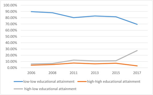
Figure 10. Inequality distribution of total household income in China: differences in marital structure.

Source: CSS survey data from 2006 to 2017.

From Figure 9, households with low–low educational attainment combined accounted for the most significant proportion, even reaching 89.81 in 2006. Although the sample proportion continued to decrease from 2006 to 2017, it still accounted for 69.47% in 2017, more than half of the total number of households. The ratio of households combined with high–high educational attainment and high–low educational attainment has increased, reaching 7.25% and 11.19%, respectively in 2015. In 2017, the proportion of households combined with high–low educational attainment had risen sharply, arriving at 27.49. This is related to the national situation of China. The illiteracy rate of the founding of New China is 80%. By 1964, the illiteracy rate was still as high as 52%. The nine-year compulsory education policy has improved the education level of the people, but many people still cannot obtain higher education. Therefore, the number of households with a low–low educational attainment combination is higher than the other two categories.

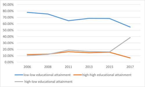
From Figure 10, we can see the proportion of the total income of households with different marriage structures. The highest proportion of total household income is the low–low educational attainment combination household. The whole household income accounted for 77.89% in 2006 and has declined year by year since then. The most significant decline was from 2008 to 2011, with a drop of almost 10%. In the next two years, the proportion of income has steadily declined, reaching the lowest point of 54.95% in 2017. The proportions of the total income of households with high–high educational attainment combination and that with high–low educational attainment combination are highly overlapped from 2006 to 2015. Still, the sample size of households with high–high educational attainment combinations is smaller than that of high–low educational attainment combinations. However, in 2017, there was a significant difference in the proportion of household income between the two structures. The household with high–low educational attainment combinations was more than 30% higher than the high–high educational attainment combination.

Comparing with Figure 9, we can see the following points: First of all, the households with low–low educational attainment are declining in both sample size and the proportion of income. The income decline is much higher than the sample size. This is the inevitable result of improving the education level of Chinese residents. As the number of people with higher educational attainment increases, homogeneity marriages with low educational attainment will naturally decrease. Second, the sample of high–high educational attainment combination households has the most negligible proportion. But the proportion of total household income is relatively high. The revenue ratio is roughly twice the sample, and the gap increases over time. Third, the proportion of households with high–low educational attainment combination, also known as households with educational heterogeneous, continues to rise. The ratio of total household income is also increasing; ratio females:males. It can be seen that the income of households with a high–low education combination is also higher than the sample size, and increased education still brings effective income increase. Households with a low–low education combination are increasingly disadvantaged in distributing total social income. Moreover, this disadvantaged position will continue to the children's descendants, further solidifying the class and widening the household income gap.

6. Conclusion

The rate of Chinese women's access to education has increased. With the economic transformation, China's marriage matching model has continued to change, the proportion of educational homogeneity marriages has increased, and household income inequality has increased too. This article uses C.S.S. data from 2006 to 2017 to first calculate the inequality of total household income and per capita household income in China using households as the unit of measurement. After calculation, the Gini coefficient of total household income in China fluctuates between 0.47 and 0.52, with the highest point being 0.5192 in 2011. The per capita household income coefficient fluctuates between 0.5 and 0.54, with the highest point being 0.5396 in 2011. This shows that the Gini coefficient of Chinese household income is relatively high.

Finally, this article uses percentile structure analysis to analyse the internal structure of household income inequality from educational homogeneity marriage. The results show that: (1) High-income households account for most of the total social income, crowding out the resources of low-income households to a certain extent, and the general social trend tends to be class solidification; (2) As the household size expands, the income gap rises. In order to cope with the increasing cost of living and reduce the marginal expenditure of life, low-income households will inevitably continue to expand the household size; (3) The total income distribution of Chinese households differs significantly in the educational attainment of household heads. A small number of highly educational attainment households occupy relatively more social wealth. The income differentiation brought about by educational attainment further exacerbates the income gap in Chinese households; and (4) Both the sample size and the income share of the low–low educational attainment combination households are declining, and the income decline is much higher than the sample size. High–high educational and high–low educational attainment combination households have gradually increased and occupy more social income.

On this basis, we believe that the government should consider the following points when conducting income regulation. (1) Develop an income security system from the household's perspective, add the total household income level to the standard of poverty measurement, and guarantee the living standards of all members of poor households; (2) The government should fully account for the income inequality caused by educational inequality in policy formulation. They are popularising higher education, lowering the financial threshold of higher education, and allowing more people to have the opportunity to choose higher education, which will not only increase national happiness but also reduce the household income gap. The spiritual pleasure and human dignity brought by education can satisfy the spiritual needs of the people; and (3) Encourage women in the family to participate in employment, improve their educational attainment during infancy, and improve the welfare and security system to liberate women from the family, reduce the income gap within the family, and alleviate the inequality of total household income.

Disclosure statement

The authors reported no potential conflict of interest.

Additional information

Funding

This study is supported by the Science and Technology Project of Jiangxi Provincial Department of Education (No. GJJ209923.

References

- Acemoglu, D. (2003). Cross-country inequality trends. Economic Journal, 113(485), F121–F149. https://doi.org/10.1111/1468-0297.00100
- Amaa, B. (2020). The effects of human capital and social factors on the household income of Bangladesh: An econometric analysis. Journal of Economic Development, 45(3), 29–49. https://doi.org/10.35866/CAUJED.2020.45.3.002
- Antonelli, C., & Gehringer, A. (2017). Technological change, rent, and income inequalities: A Schumpeterian approach. Technological Forecasting and Social Change, 115, 85–98. https://doi.org/10.1016/j.techfore.2016.09.023
- Atkinson, A. B., & Bourguignon, F. (2000). Introduction: Income distribution and economics. Handbook of Income Distribution, 1, 1–58. https://doi.org/10.1016/S1574-0056(00)80003-2
- Baum-Snow, N., & Pavan, R. (2013). Inequality and city size. The Review of Economics and Statistics, 95(5), 1535–1548. https://doi.org/10.1162/REST_a_00328.
- Bertrand, M., Goldin, C., & Katz, L. F. (2010). Dynamics of the gender gap for young professionals in the financial and corporate sectors. American Economic Journal: Applied Economics, 2(3), 228–255. https://doi.org/10.1257/app.2.3.228
- Breen, R., & Salazar, L. (2011). Educational assortative mating and earnings inequality in the United States. American Journal of Sociology, 117(3), 808–843. https://doi.org/10.1086/661778
- Cao, T., & Qian, X. (2021). Political capital and household income: Evidence from twenty-four transition countries. Journal of Family and Economic Issues, 42(1), 151–165. https://doi.org/10.1007/s10834-020-09708-6
- China Household Finance Survey and Research Center. (2012). The Southwestern University of Finance and Economics report on China's household income inequality in China. Chengdu: Southwestern University of Finance and Economics Press.
- Chotikapanich, D., Rao, D. S. P., & Tang, K. K. (2007). Estimating income inequality in China using grouped data and the generalized beta distribution. Review of Income and Wealth, 53(1), 127–147. https://doi.org/10.1111/j.1475-4991.2007.00220.x
- Duranton, G., & Puga, D. (2004). Micro-foundations of urban agglomeration economies. In J. Vernon Henderson & Jacques François (eds.), Handbook of regional and urban economics, Working Paper 9931 (Vol. 4, pp. 2063–2117). North Holland: Elsevier. http://www.nber.org/papers/w9931.
- Eika, L., Mogstad, M., & Zafar, B. (2019). Educational assortative mating and household income inequality. Journal of Political Economy, 127(6), 2795–2835. https://doi.org/10.1086/702018
- Esping-Andersen, G. (2007). Sociological explanations of changing income distributions. American Behavioral Scientist, 50(5), 639–658. https://doi.org/10.1177/0002764206295011
- Gordon, R. J., & Dew-Becker, I. (2008). NBER working paper series controversies about the rise of American inequality: A survey. http://www.nber.org/papers/w13982
- Greenwood, J., Guner, N., Kocharkov, G., & Santos, C. (2014). Marry your like: Assortative mating and income inequality. American Economic Review, 104(5), 348–353. http://dx.doi.org/10.1257/aer.104.5.348
- Grow, A., & Van Bavel, J. (2020). The gender cliff in the relative contribution to the household income: Insights from modelling marriage markets in 27 European countries. European Journal of Population = Revue Europeenne de Demographie, 36(4), 711–733. https://doi.org/10.1007/s10680-019-09547-8.
- Haigang, W. (2005a). Income changes of Chinese households and their impact on long-term equality. Economic Research, (01), 56–66.https://kns.cnki.net/kcms/detail/detail.aspx?FileName=JJYJ200501005&DbName=CJFQ2005
- Haigang, W. (2005b). Intergenerational mobility of Chinese residents' income distribution. Economic Science, (2), 18–25. https://doi.org/10.19523/j.jjkx.2005.02.002
- Haigang, W., & Kaiguo, Z. (2006). Is the inequality of income distribution between urban and rural residents in China underestimated? – A test based on Pareto distribution. Statistical Research, (04), 8–15. https://doi.org/10.19343/j.cnki.11-1302/c.2006.04.002
- Han, L. (2010). A review of income inequality: An empirical study in China, 2000-2009. Social Science Column, 25, 35–37.
- Jinbao, Z., & Li, L. (2013). Research on the measurement method of urban household income distribution and Gini coefficient based on interval data. Quantitative and Technical Economic Research, 30(7), 116–130. https://doi.org/10.13653/j.cnki.jqte.2013.07.020
- Jinghui, D., & Jianbao, C. (2010). Measurement of the regional Gini coefficient based on household income distribution and its urban-rural decomposition. World Economy, 33(01), 100–122.
- Kremer, M. (1997). How much does sorting increase inequality? The Quarterly Journal of Economics, 112(1), 115–139. https://doi.org/10.1162/003355397555145
- Lang, K., & Lehmann, J.-Y. K. (2011). NBER working paper series racial discrimination in the labor market: Theory and empirics. http://www.nber.org/papers/w17450
- Liqun, P., Jing, L., & Jiafeng, Z. (2015). Education homogeneity mating and family income inequality. China Industrial Economy, (08), 35–49. https://doi.org/10.19581/j.cnki.ciejournal.2015.08.003
- McDonald, J. B., & Jensen, B. C. (1979). An analysis of some properties of alternative measures of income inequality based on the gamma distribution function. Journal of the American Statistical Association, 74(368), 856–860. https://doi.org/10.1080/01621459.1979.10481042
- Mon, Y. Y., & Kakinaka, M. (2020). Regional trade agreements and income inequality: Are there any differences between bilateral and plurilateral agreements? Economic Analysis and Policy, 67, 136–153. https://doi.org/10.1016/j.eap.2020.07.003
- Moretti, E. (2004). Chapter 51 Human capital externalities in cities. In J. V. Henderson & J. F. (eds.), Handbook of regional and urban economics (Vol. 4). Elsevier Inc. https://doi.org/10.1016/S1574-0080(04)80008-7
- Piketty, T. (2017). Capital in the twenty-first century. Harvard University Press. https://doi.org/10.4159/9780674982918
- Qiongzhi, L., & Qin, L. (2015). Estimation of China's household income inequality: The measurement of hidden income and the choice of income distribution function based on grouped data. Zhongnan Economic and Economic Law University, 208(1), 3–11.https://kns.cnki.net/kcms/detail/detail.aspx?FileName=ZLCJ201501001&DbName=CJFQ2015.
- Qiuchuan, J. (2018). The impact of education matching in marriage on China's income gap. Journal of Zhongnan University of Economics and Law, 227(02), 32–42. https://doi.org/10.19639/j.cnki.issn1003-5230.2018.0018
- Schmittlein, D. C. (1983). Some sampling properties of a model for income distribution. Journal of Business & Economic Statistics, 1(2), 147–153. https://doi.org/10.1080/07350015.1983.10509333
- Shi, L. (2015). The change and reform of China's income distribution pattern. Journal of Beijing Technology and Business University (Social Science Edition), 30(7), 1–6. https://doi.org/10.16299/j.1009-6116.2015.04.001
- Xie, Y., & Zhou, X. (2014). Income inequality in today’s China. Proceedings of the National Academy of Sciences of the United States of America, 111(19), 6928–6933. https://doi.org/10.1073/pnas.1403158111.
- Xinjian, H., & Jinchang, L. (2005). How to correctly measure the Gini coefficient of Chinese residents' income. Nankai Economic Research, (04), 53–57. https://kns.cnki.net/kcms/detail/detail.aspx?FileName=NKJJ200504010&DbName=CJFQ2005
- Xiwei, W. (2011). Inequality of income and property of Chinese urban households: 1995–2002. Population Research, 35(06), 13–26.
- Zexia, W., Xiaoxin, Z., & Limin, N. (2011). China's interprovincial rural household income inequality: Regional decomposition based on the “Gini” coefficient. Economic Issues Exploration, 2011(04), 17–21.
- Zhijun, H. (2012). Estimation of Gini coefficient and social welfare based on subgroup data: 1985–2009. Research in Quantitative Economics and Technical Economics, 29(09), 111–121.