A model proposal for IFRS 16 IBR adjustment based on bond market pricing

Abstract

The Incremental Borrowing Rate (IBR) is generally used by companies for discounting future lease payments and calculating the value of the lease assets and liabilities under IFRS 16. According to this standard, leased asset must be considered as a collateral, and therefore the yield to be used should reflect an adequate Loss-Given Default (LGD), which may vary depending on the estimated recovery rate of the asset (machinery, real estate, vehicles, etc.). There is a lack of accounting and finance literature focused on analysing how a standard IBR should be adjusted to reflect the expected underlying asset LGD in line with IFRS principles. In this context, we propose a model that uses bond quoted information as a basis for introducing an adjustment to the standard “unsecured” IBR. The model consists of replicating the change in a certain bond yield when there is a change in the LGD (usually due to a change in the seniority level). We empirically demonstrate that the model works by using data from real bond quotations (97 outstanding bonds quoted on several secondary markets such as NY, Vienna, Frankfurt and London). The empirical analysis has been performed for two different time periods: pre-COVID 19 and post-COVID 19.

Keywords:

• IFRS 16
• Incremental Borrowing Rate (IBR)
• Loss Given Default (LGD)
• Yield-to-Maturity (YTM)
• bond pricing

JEL Classification:

• C13
• C52
• G12
• G33
• M41

1. Introduction

In 2016, the International Accounting Standards Board (IASB) issued a new lease standard (International Financial Reporting Standard - IFRS − 16) that came into effect for reporting periods beginning on or after January 1, 2019. This standard replaced IAS (International Accounting Standard) 17 that had been regulating lease operations since 1994 and that was issued by the former International Financial Standards Committee (IASC). This represents one of the most significant changes in accounting rules to have taken place over the last 40 years, having a great impact on companies’ reporting of debt levels and on many financial ratios (Morales-Díaz & Zamora-Ramírez, 2018a and 2018b).

IFRS 16 introduced an important change in the accounting model to be applied by lessees, leaving the lessors’ model basically unchanged in relation to IAS 17. Under the previous standard, lessees had to classify all lease agreements in two categories: operating and finance leases. If the lease was classified as an operating lease, the lessee simply recognized a lease expense over the lease term (without recognizing assets or liabilities on the balance sheet)¹. If the lease was classified as a finance lease, the lessee recognized the leased good on the asset side as if the entity was the legal owner (subject to amortization and impairment), as well as a debt on the liability side (along with the corresponding interest expenses). In other words, finance lease operations were basically accounted for as financed purchases of the underlying asset. In fact, in the finance lease model, the “substance over form principle” was implicit. Morales-Díaz et al. (2019) analyze how the accounting principle known as “substance over form” has been generally applied in lease accounting since the beginnings of modern accounting regulation.

Under IFRS 16, the distinction between operating and financial leases disappeared for lessees², and instead a new capitalization model is applied for all lease transactions (apart from certain voluntary exceptions³). This capitalization model basically consists of initially recognizing an asset (called “right-of-use”) and a liability (called “lease liability”). The asset is subject to amortization and impairment, and the liability is accounted for as an amortized cost debt. The basic difference between this capitalization model and the former finance lease model is that the capitalization model is only applied to the “right-of-use” i.e., to the part of the useful life of the underlying asset that is transferred to the lessee and not to the whole asset.

In order to calculate the initial value of the lease asset and lease liability under IFRS 16, the entity must discount future lease payments over the lease term. The discounting of lease payments can be done using two alternative rates (IFRS 16, parr. 26): the lease implicit rate or the lessee’s incremental borrowing rate (hereinafter, IBR). IBR can be used in cases in which the lease implicit rate cannot be calculated by the lessee.

The interest rate implicit in the lease, is “the rate of interest that causes the present value of (a) the lease payments and (b) the unguaranteed residual value to equal the sum of (i) the fair value of the underlying asset and (ii) any initial direct costs of the lessor” (IFRS 16 Appendix A, Supplementary material).

The IBR is the rate of interest that a lessee would have to pay to borrow over a similar term, and with a similar security, the funds necessary to obtain an asset of a similar value to the right-of-use asset in a similar economic environment.” In other words, it would correspond to the rate of a hypothetical loan issued by the lessee in other to buy the underlying asset or, more precisely, the right of use of the underlying asset over the lease term.

As pointed to by Deloitte (2018, p. 6) and KPMG (2017, p. 11), on most lease contracts, the lease implicit rate cannot be obtained because there is not enough information (IFRS 16, parr. BC 161). Therefore, in order to apply the IFRS 16 capitalization model, entities must estimate an IBR for most lease operations in which they act as a lessee, and in which the voluntary exceptions do not apply. The IBR was also used under previous lease standard IAS 17. Blum and Thérond (2019) point out that a discount rate is used in many IFRS standards. They find that definition is not consistent among them, and not all of them are consistent with finance theory. The authors also conduct a survey of 30 European accountants, CFOs, auditors and executives with financial functions covering a variety of topics in relation to discount rates in IFRS. Their results show how the entities and the auditors have to face many challenges in order to comply with IFRS discount rates, and how there is wide diversity in practice.

Moreover, IFRS 16 IBR has an additional difficulty as compared to other accounting discount rates. The standard establishes that when estimating the IBR, the entity should consider not only the credit quality of the issuer (the lessee), but also the fact that that the hypothetical loan (for which the rate is obtained) is guaranteed by the underlying asset. This is due to the fact that if the lessee does not comply with its payments (under the lease contract), then the lessor has the right to recover the leased asset and, therefore, it does not lose the complete remaining theoretical nominal amount. The credit risk of the lease contract is, therefore, generally lower than that of an unsecured loan. In this regard, the type of underlying asset (real estate, vehicles, machinery, etc.) should also be considered: the higher its estimated value, the higher the recovery rate and the lower the discount rate will be.

It may be quite simple to estimate an initial hypothetical rate using data from an unsecured loan or bond issued by the company or by peer companies (Step 1) (IFRS, 2019, p.6). Nevertheless, this initial yield should be adjusted in order to reflect the correct recovery rate associated with the underlying asset (Step 2). According to the IFRS Interpretations Committee, “in determining its incremental borrowing rate, the Board explained in paragraph BC162 that, depending on the nature of the underlying asset and the terms and conditions of the lease, a lessee may be able to refer to a rate that is readily observable as a starting point. A lessee would then adjust such an observable rate as is needed to determine its incremental borrowing rate as defined in IFRS 16” (IFRIC, 2019)⁴.

The analysis required to adjust Step 1 yield to Step 2 yield may prove to be complicated since:

1. Generally speaking, entities are not able to find quoted assets (bonds) linked to the various recovery rates that are associated with the different, plausible underlying assets backing a leasing contract (vehicles, machinery, equipment, real estate, etc.). Therefore, there is no direct market reference, and a two-step process is necessary (i.e., the two steps mentioned above).

2. IFRS 16 (nor other accounting standards) do not establish or describe a technique for Loss Given Default (LGD⁵) adjustment.

3. Currently entities do not disclose how they make said adjustment, and the majority do not actually disclose if they make the adjustment or not. We have analyzed the financial statements of European listed companies from the retail and hotel sectors (sectors with a higher IFRS 16 impact, see Morales-Díaz & Zamora-Ramírez, 2018b) (74 companies in total). In the notes to their financial statements, only 33.8% of the companies disclose their adjustment of the IBR considering the leased asset as a collateral, with similar ratios by industry. However, none of them disclose how they make said adjustment.⁶

4. As we will see in Section 2, there is little in the previous literature regarding how a standard yield curve may be adjusted in order to reflect the correct LGD using a simple model that can be applied by financial statement preparers and that also comply with IFRS 16 requirements.

In relation to this last point, the existing literature does widely cover the LGD adjustment for loan pricing (Luck & Santos, 2022; Akguen & Vanini, 2007), the measuring of loan loss provisioning (Frontczak & Rostek, 2015), or the estimating of the Credit/Debit Value Adjustment (CVA/DVA) in derivatives valuation (Yashkir & Yashkir, 2013; Qi & Zhao, 2011; Bastos, 2010). There is even a research line for estimating the real LGD for lease operations (Hartmann-Wendels et al., 2014; Miller & Töws, 2018). Nevertheless, the literature offers no examples of a proposed model linking the LGD with the yield to be used in the context of IFRS 16 (the IBR). In other words there are no proposals for a model for Step 2 adjustment as explained above.

In this article, we develop a model that serves to fill both the practical and theoretical gaps. The model basically consists of replicating the change in a certain bond yield when there is a change in the LGD (usually due to a change in the seniority level). Moreover, we empirically demonstrate that the model functions by using real market data of quoted bonds, i.e., we apply our model to a real sample of quoted bonds, and subsequently analyze—over two different time periods, namely pre-COVID 19 and post-COVID 19—whether the model predicts the change in YTM⁷ when a change in the recovery rate occurs.

This work contributes to the previous literature in three main aspects. First, it can be used for future research about the impact of lease accounting rules. Previous studies use a unique rate for discounting lease payments (Beattie et al., 1998; Bennett & Bradbury, 2003; Duke et al., 2009; Ely, 1995; Imhoff & Lipe, 1997; Singh, 2012; Wong & Joshi, 2015). It can be used also for discount pensions and other provisions (Fülbier et al., 2008; Pardo & Giner, 2017); or as a benchmark rate plus a firm credit spread (Durocher, 2008; Fitó et al., 2013). Second, several models have been developed for estimating the LGD (with a given sample of loans at a certain date) (Akguen & Vanini, 2007; Silaghi et al., 2020), but none present a model to explain how a standard yield curve can be adjusted in order to reflect the correct LGD. Finally, our model can be used by IFRS 16 practitioners in order to adjust “standard” IBR to the IBR applicable to different lease assets associated with different LGDs. Besides, this model is also applicable for estimating the fair value of a loan/bond that includes an asset as a collateral, and the calculation of the interest rate of a collateralized loan transaction between a lender and a borrower.

The remainder of this article is structured as follows: Section 2 contains a review of the previous literature. In Section 3, we provide an explanation of the proposed model, including the hypotheses and theoretical basis, along with a practical example of how it may be applied. Section 4 includes the empirical analysis, while Section 5 details our conclusions.

2. Previous literature

2.1. The role of the collateral in bond pricing

There is extensive previous literature regarding the LGD (the role of the collateral in different types of lending agreements) in several contexts, mainly focussed on loan/bond pricing; the measuring of loan loss provisioning; and on estimating the CVA/DVA adjustment for derivatives valuation.

According to the finance literature, there are two possible theories as to why lending agreements include collateral:

1. Asymmetric information theory. This theory assumes that, on entering a loan operation, the borrower has generally more information than the lender in relation to its own credit situation. If, in this context, the borrower knows that its credit quality is poor, it offers to pledge collateral as a potential signal of lower risk. This argument has been proposed and analyzed by Besanko and Thakor (1978,2020b) and by Chan and Kanatas (1985).

2. Lender requirement. According to this theory, the lender is generally the party that, having analyzed the borrower’s credit quality, requires collateral for mitigating the risk. This argument has been analyzed by Berger and Udell (1990), and for the most part, the majority of empirical evidence has supported this theory (Luck & Santos, 2022).

In our specific case (lease contracts), collateral is included in the contract due to the nature of the agreement itself and not because either of the parties has requested a certain asset to be pledged. If the lessee fails to pay the corresponding quotes, the lessor (who is the legal owner of the leased asset) will repossess the asset. In this sense, the lessor will recover the nominal amount of the theoretical loan (or part of it, depending on the “loan to value”) and will only lose the unpaid quotes. Therefore, the abovementioned theories do not apply to lease contracts.

In relation to loan/bond pricing literature, we can highlight several works given the relationship they have with the model that we propose in Section 3. First, all bond pricing methodologies consider the recovery rate/LGD in one form or another, since it is an important factor that affects the price. This is one of the bases of our model, i.e., that the bond price changes when there is a change in the LGD. When using a closed-formula for bond pricing, authors generally consider the recovery rate to be a constant or an exogenous variable that is estimated using market data (Jarrow & Turnbull, 1995; Duffie & Singleton, 1999). For example, Duffie and Singleton (1999) derived an approximate pricing formula for defaultable bonds. Under their evaluation framework, the value of a defaultable bond is calculated by a default-adjusted rate. This rate comprises the default-free short interest rate process and a mixed process, which is the product of the default intensity rate and the loss rate. Chiang and Tsai (2010) developed a model in which the recovery rate is considered a stochastic variable. Moreover, default probabilities and recovery rates can be derived from bond prices (Sections 3 and 4) (Ando, 2014; Spuchľakova & Cug, 2015).

Many authors have empirically analyzed the direct influence of the recovery rate (value of the collateral) on loan/bond pricing. In one of the most recent studies, Bellucci et al. (2021) use a variety of estimation methods in order to explore the empirical relationship between interest rates and collateral requirements in bank loan contracts, and conclude that there is a strong relationship between the loan interest rate and the collateral, and that the higher the value of the collateral, the lower the interest rate will be. Luck and Santos (2022) demonstrated the influence of different types of collateral in loans spreads, being marketable security collaterals the most valuable. Benmelech and Bergman (2009) find that debt tranches that are secured by more redeployable collateral carry lower credit spreads, higher credit ratings, and higher loan-to-value ratios, thereby confirming that pledging collateral is valuable. Cerqueiro et al. (2016) also confirm loans whose collateral was affected by a law change experienced a greater increase in pricing compared to loans with unaffected collateral. The influence of LGD in the interest rate of loans has been also demonstrated in Duo and Meder (2020), Lara-Rubio et al. (2017), Matias and Dias (2015), Benmelech and Bergman (2011), and Bo (2020). As concluded by Blazy and Weill (2013) and Gonas et al. (2004), the collateral reduces the lender’s loss should the borrower default on the loan leading us to propose a model which the standard curve increases the yield as the relative value of the collateral (the lease asset) decreases, and vice versa. Specifically, our model transfers the change in bond yields to the yield curve, when a change in the recovery rate occurs.

As previously stated in Section 1, the previous literature does not include any model which shows how a standard yield curve can be adjusted in order to reflect the correct LGD. Other models do exist, but these study bond price responses to rating variations (Miao et al., 2014), or liquidity movements (Uhrig-Homburg & Kempf, 2000). Akguen & Vanini, 2007 introduce a framework in order to analyze the joint impact of credit risk and market risk of collateral on loan pricing. They obtain a semi-analytic expression for the values of loans, and for the value of credit protection emanating from the collateral.

2.2. LGD for lease operations

Hartmann-Wendels et al., 2014 and Miller and Töws (2018), estimate the recovery rate in lease operations according to the type of leased asset. They use a dataset from three German leasing companies with 14,322 defaulted leasing contracts in order to analyze different approaches to estimating the Loss Given Default (LGD). As a global average, the LGD is approximately 39.5% for vehicles; 49% for machinery; 88.2% for ICT; 66% for equipment; and 46% for others. The findings of these studies can be used by companies for the estimation of the recovery rates of the different leased assets for the purpose of applying our proposed model.

2.3. IFRS discount rates

Some research does already exist in relation to IFRS discount rates, but there is none specifically dedicated to IFRS 16 (or, previously, to IAS 17). Rather, the research focuses on other standards in which the discount rate also plays an important role as IAS 36 (“Impairment of Assets”) and IAS 37 (“Provisions, Contingent Liabilities and Contingent Assets”).

IAS 36 gives the entity the choice of three different starting points to calculate the discounting factor for impairment. Husmann and Schmidt (2008) demonstrate that the weighted average cost of capital (WACC) is the only suitable starting point for all scenarios. But the WACC is not suitable for calculate IBR, because includes the cost of capital, and the cost of capital is different to the cost of debt according to IFRS 16.Carlin and Finch (2009, 2010) focus on the discount rate in goodwill impairment testing under IAS 36, concluding the discretion surrounding rate selection could be used opportunistically to avoid or manage the timing of impairment losses to the detriment of transparency, comparability and decision usefulness.

Michelon et al. (2020) and Schneider et al. (2017) focus on the discount rates used when applying IAS 37, finding there is significant diversity in practice in terms of both discount rate choices and related disclosures across industry sectors as well as countries. The choice of these discounting rates can be used opportunistically avoiding a major increase in environmental liabilities.

Blum and Thérond (2019) find that the discount rate is used in many standards across the different IFRS. The definition is not consistent among them, and not all of them are consistent with finance theory. Conducting a survey of 30 European accountants, CFO, auditors and executives with financial functions, their results show how the entities and the auditors have to face many challenges in order to comply with IFRS discount rates, and how there is a wide diversity in practice. While IFRS 16 is mentioned, there are no specific references as to how entities comply with IFRS 16. We will attempt to fill this gap in the literature with this study.

2.4. IFRS 16 specific

Finally, IFRS 16-specific literature has been focused on the effects of IFRS 16 on companies’ financial statements, and more precisely on the impact of implementing a lease capitalization model (Bennett & Bradbury, 2003; Duke et al., 2009; Durocher, 2008; Fitó et al., 2013; Fülbier et al., 2008; Goodacre, 2003; Grossman & Grossman, 2010; Imhoff & Lipe, 1991 and 1997; Mulford & Gram, 2007; Singh, 2012). These studies were developed under a draft standard. Several papers predicted impacts on lease capitalization models based on previous financial statements, and also estimated further impacts on future statements (Morales-Díaz & Zamora-Ramírez, 2018b; Giner et al., 2019).

To date, however, there are still no studies which analyze the true impact of actual IFRS 16 implementation. It can be easily seen that the impact has been very significant—it suffices to compare the debt level of a company from the retail, hotel, transport sectors etc. before and after IFRS 16 implementation.

3. Model proposal and theoretical basis

3.1. Introduction and previous information to be obtained by the preparers of financial statements

Our proposed model is developed within a default risk pricing framework, and the relationship between default probability, recovery rates and YTM. Our main objective is to develop a model that allows an existing “standard” borrowing rate (the standard IBR/YTM) (Step 1 as explained in Section 1) to be adjusted in order to obtain a new rate that implicitly reflects the expected recovery rate of the underlying asset (collateral) (Step 2 as explained in Section 1). In line with the previous literature (Section 2.1 above), the adjustment to the initial yield should be performed in such a way that higher recovery rates will entail lower yields, and vice-versa.

Before introducing the model itself, consideration must be given to the fact that entities need to obtain two specific data prior to applying the model:

1. A “standard” IBR/YTM for a certain date (or a standard curve if we consider several maturities) (Step 1 as explained in Section 1). Generally, as we will see, this standard IBR/YTM assumes a recovery rate of 40%.

2. The expected recovery information for the leased assets.

With regard to the appropriate standard discounting curve, if the lessee maintains issued quoted debt or bonds, then this curve can be constructed using this information. Should this not be the case, additional analyses should be undertaken in order to calibrate a curve that can be associated with the lessee’s rating and sector under a standard seniority (usually senior unsecured debt). See, for instance, the work of Delgado-Vaquero and Morales-Díaz (2018) and Delgado-Vaquero et al. (2020) containing proposed models for estimating a theoretical credit rating for an entity that does not have an official credit rating.

Recovery information (the recovery rate) is the other critical data needed to be obtained. Under normal circumstances, standard market information related to loan and bonds recovery rates may be easily obtained as regards the main sectors, covering historical data on LGDs. This information is usually provided by the principal rating agencies. Most quoted debt instruments (and their linked standard yield curves) are senior unsecured bonds, with a standard recovery rate of approximately 40%, according to historical performance adopted to price standard credit-linked instruments (bonds, CDS and other credit derivatives) by market conventions.

In Table 1 below, we present the average recovery rates for debt instruments that defaulted in recent years (according to data from Moody’s), and we compare them with historical averages. We categorized the information provided on the recovery rates by priority position (from 1st lien bank loans down to junior, unsecured and subordinated securities). It can be seen that over the past three decades, recovery rates have generally been correlated with seniority in the debt structure of the issuer. In this regard, seniority refers to a higher average recovery rate. For example, first lien bank loans (loans with higher seniority) have the highest average recovery rate (around 67%). This result is logical given their secured nature and their seniority within the debt structure, and is coherent with previous literature (Section 2 above).

Table 1. Average corporate debt recovery rates measured by trading prices.

Priority Position	Issuer-weighted recoveries
	2017	2016	1983–2017
1st Lien Bank Loan	69.04%	75.05%	67.07%
2nd Lien Bank Loan	17.87%	22.50%	30.38%
Sr. Unsecured Bank Loan	9.00%	n.a.	45.87%
1st Lien Bond	62.43%	48.72%	53.62%
2nd Lien Bond	52.75%	34.07%	45.18%
Sr. Unsecured Bond	53.85%	31.45%	37.74%
Sr. Subordinated Bond	38.00%	36.72%	31.10%
Subordinated Bond	74.38%	24.50%	32.05%
Jr. Subordinated Bond	17.50%	0.63%	22.79%

Source: Moody’s (2018).

The recovery data shown above is based on trading prices “at default” or “post default.” An alternative recovery measure is based on ultimate recoveries, i.e., the value that creditors recover once the default event is resolved (Table 2). For example, in the case of issuers filing for bankruptcy, the ultimate recovery is the present value of the cash or securities that creditors actually receive when the issuer’s bankruptcy is legally finalized, typically one to two years after the initial default date.

Table 2. Average corporate debt recovery rates measured by ultimate recoveries, 1987–2017.

Priority position	Emergence year			Default year
	2017	2016	1987–2017	2017	2016	1987–2017
Loans	81.3%	72.6%	80.4%	80.2%	78.3%	80.4%
Senior Secured Bonds	52.3%	35.9%	62.3%	57.5%	46.9%	62.3%
Senior Unsecured Bonds	54.1%	11.7%	47.9%	47.4%	29.2%	47.9%
Subordinated Bonds	4.5%	6.6%	28.0%	n/a	8.0%	28.0%

Source: Moody’s (2018).

From Table 1 and Table 2, it can be seen that senior, unsecured bonds are mostly assumed to have an average recovery rate, from a historical perspective, of approximately 40%. This recovery rate is aligned with the multiple recovery rates present on the credit market by issuer’s rating for Senior, Unsecured bonds, for a relevant time horizon (Table 3).

Table 3. Average senior unsecured bond recovery rates by year prior to default, 1983–2017.

Issuer’s rating	Year 1	Year 2	Year 3	Year 4	Year 5
Aaa		3.33%	3.33%	61.88%	69.58%
Aa	37.24%	39.02%	38.08%	43.95%	43.18%
A	30.36%	42.57%	44.97%	44.49%	44.17%
Baa	42.89%	44.16%	43.99%	43.79%	43.52%
Ba	44.63%	43.30%	42.13%	41.60%	41.59%
B	37.62%	36.77%	37.21%	37.71%	38.36%
Caa-C	38.10%	38.43%	38.50%	38.83%	38.86%
Investment Grade	40.04%	43.33%	43.96%	44.11%	43.86%
Speculative Grade	38.34%	38.19%	38.31%	38.66%	38.99%
All Rated	38.40%	38.47%	38.71%	39.11%	39.45%

Source: Moody’s (2018).

The fact that a senior, unsecured bond is expected to have a recovery rate of approximately 40% is relevant to our model proposal, as will be subsequently explained in Sections 3.2 and 3.3.

This background serves as the underlying basis for our model. As may be expected, lease collaterals generally have different recovery rates (not necessarily 40%), given their specific nature, expected value, asset usage and expected amortization. Table 4 below summarizes real data gathered from leasing collaterals and their respective recovery rates:

Table 4. Estimated recovery rates for leasing contracts.

Leased asset	Recovery Rate
Vehicles	60.47%
Machinery	50.91%
ICT	11.79%
Equipment	33.96%
Other	53.98%

Source: Hartmann-Wendels et al. (2014) and Ou et al. (2016).

Nonetheless, as previously stated, quoted products do not exist in markets that are linked to the different recovery rates associated with the underlying assets backing a leasing contract. So, we need to introduce in the model risk as yield-to-maturities, credit ratings, recovery rates, credit spreads, default probabilities and updated market information.

3.2. Model hypotheses

Generally, entities cannot observe in the market the quoted price of traded bonds or other fixed income products with are similar (in terms of probability of default, maturity, etc.) and that are linked to different recovery rates. In this sense, our model is based on analyzing the theoretical change in a certain quoted product (a bond) when the recovery rate changes. That change can, then, be transferred to the initial standard curve based on the applicable LGD.

Our model is based on the following hypotheses and assumptions:

1. We are assuming a static and deterministic probability of default curve for all recovery rate levels (Jarrow & Turnbull, 1995; Duffie & Singleton, 1999; Chiang & Tsai, 2010).

2. We are assuming that the credit quality of the lessee can be estimated (through an official or unofficial credit rating). The unofficial credit rating and be obtained using the financial information issued by the lessee.

3. The recovery rate (R) is basically determined by the seniority and the type of collateral. The higher the seniority and the better quality of the collateral, the higher the estimated recovery rate. In general, bonds and CDS quotes assume a standard recovery rate of 40% (unsecured debt) (Moody’s, 2018).

4. Current losses-given default cannot be predicted by neither long-term averages nor moving averages of loss-given. LGD have a cyclical nature and, therefore, can vary throughout time depending on the general situation of the economy (EBA, 2017)⁸.

5. The debt that is unsecured is, generally, more sensitive to the default risk and to the general state of the economy that the debt that is secured. In this sense, products secured with more liquid collaterals generally have higher recovery rates than those secured with less liquid collaterals Benmelech & Bergman, 2009; Cerqueiro et al., 2016, Duo & Meder, 2020; Lara-Rubio et al., 2017; Matias & Dias, 2015, Moody’s, 2018).

6. The most relevant sources of financial information are fixed income and credit markets. The relationship between LGDs, yields-to-maturity and default risk is understood through market instruments (Schonbucher, 2003).

7. Our model does not consider factor like the liquidity of the risk contract itself or like sovereign risk.

3.3. Model Proposal: bond price and YTM sensitivity to recovery rate

Our proposal is based on the pricing of traded debt instruments issued by the lessee (or similar peers in terms of rating and sector) following a default-tree model. A binomial tree can be constructed in order to calculate the debt instrument’s value at each tree node, taking into account the conditional default probabilities $\left[{SP}_i-{SP}_{i-1}\right]$ existing at each node $i,$ as it is shown in Figure 1.

where $CF(t_{i-1},t_i)$ is the risk-free cash-flow to be paid by the instrument; $SP(0,t_i)$ is the survival probability of the product between $t_0$ and$\mathrm{ }{t}_i;$ $1-SP(0,t_i)$ is the default probability for the same period; and R$R\left(t_{\mathrm{i}-1},T_i\right)$ is the estimated recovery rate of the debt instrument for each period.

Figure 1. Default-tree model.

Source: compiled by the authors

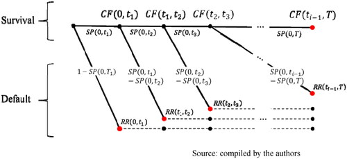
This tree shows that bonds payments have a survival probability at each node $t_i,$ but they are complemented with their default probability at the same node, where the payment value will be the only estimated recovery. That is to say, at every node $t_i$ a default event may occur, or the obligor will continue until the next date${ t}_{i+1}.$ Following default, the non-defaulted path continues (indicated by the upper continuation of the tree), but the defaulted security only earns, for a certain node, its recovery payoff and ceases to exist from there on (represented by dashed lines). The sum of the payment scenarios (indicated by red dots), weighted by the probability of their occurrence, is equal to the instrument fair value. The aforementioned also means that the probabilities attached to the branches of the tree are only the conditional default and survival probabilities at this node as seen from t = valuation date. Therefore, under the above model, the defaultable debt instrument price is as follows: (1) $$\begin{array}{c}\mathit{Fair}\mathit{Valu}{e}_{t_0}=\sum _{i=1}^{T}CF(t_{i-1},t_i)P(0,t_i)SP(0,T)+\}\text{Default}-\text{free}\mathrm{ }\text{cash}-\text{flows}\\ +\sum _{i=1}^T[RR(t_{i-1},t_i)CF(t_{i-1},t_i)[SP(0,t_{i-1})-SP(0,t_i)]]P(0,t_i)\}\text{Sum of the}\mathrm{ }\text{defaultable}\mathrm{ }\text{cash}-\text{flows}\mathrm{ }\text{recovery}\end{array}$$(1) where $CF$ is the default-free cash flow at each node i, and $P\left(0, t_i\right)$ is the risk-free discount factor.

We can assume (given the objective of the model) that default event (hazard) rates ${\lambda }_{t_i}$ for different predefined time intervals [t_i-1; t_i] of the instrument life are deterministic and constant, so that the instrument survival probability between each time interval is: (2) $$SP\left[0,t_i\right]=e^{\left(-\lambda t_i\right)}$$(2)

Hence, if we already know the market price (fair value) of the product and the recovery rate linked to its seniority, we can carry out an initial calibration of the factor $\lambda$ to the instrument market price. This is the market price (fair value) as shown in (1). Once the hazard rate has been calibrated, then all the risk factors of this model have been defined as in (1): $\mathit{Bond} \mathit{market} \mathit{value}=f\left[CF, \lambda , RR, { P(0, t}_i)\right].$ Therefore, we can analyze the sensitivity of the price to the recovery rate as follows:

• We already possess a bond’s market price with the implied hazard rate, and we will assume that the hazard rates are constant, and therefore, $SP$ only increases over time.

• Once the default-tree has been constructed, the initial recovery rate R$R$ may be changed to the chosen recovery rate estimated upon the collateral backing the leasing contract.

• Hence, this change in the RR implies a change in the bond price and, therefore, in the bond price sensitivity to the Recovery Rate, assuming that there is no immediate correlation between Recovery Rates and probability of default (although it does exist in the long-term).

• The price change can be translated into the Yield-to-Maturity or curve change, following the general framework of bond pricing: (3) $$\mathit{ond}\mathrm{ }\mathit{market}\mathrm{ }\mathit{value}=\mathrm{ }\sum _{i=1}^n{C{F}_t}_i{\mathrm{ }B(0,\mathrm{ }t}_i)$$(3)

where (4) $${\mathrm{ }B(0,\mathrm{ }t}_i)=\frac{1}{{\left(1+\mathit{YTM}\right)}^{t_i}}$$(4)

The new bond price will be given by $f\left[CF,\mathrm{ }\lambda ,\mathrm{ }RR(\mathit{new}),\mathrm{ }{\mathrm{ }P(0,\mathrm{ }t}_i)\right]$ following (1), and subsequently the implied change in the Yield-to-Maturity ($\Delta \mathit{YTM}$) will be obtained by calibrating the YTM to the new bond price, following (3) and (4).

The following example reflects how this model works.

Our scenario assumes a senior unsecured bond corresponding to a certain issuer that matures in 2025. We know that today’s bond market mid-price is 99.50%, paying a semiannual coupon of 3% with bullet amortization. The coupon payments will be made on every 30^th September and every 31^st March, and the valuation date is 30/09/2021. The nodes of the tree correspond to the payment times, for simplification purposes. $P\left[0,t_i\right]$ will be constructed by using the EONIA curve as at the valuation date.

Assuming that the recovery rate for the bonds is 40%, the default tree can be constructed as of 30/09/2021, while the hazard rate required to obtain the bond market price (99.50%) must be calibrated, following (1) and (2), against said market price. Calibrating ${\lambda }_i$ results in an implied hazard rate of 6.0875%, and the final tree would be as follows:

As a result, we obtain the bond market price which has been computed from the tree by using its corresponding recovery rate (40%) and by calibrating its implied hazard rate.

Table 5 above represents the value of each tree branch and its probability occurrence, in line with Figure 1 and (1). For instance, the first default node has a cash-flow NPV of 40.27% (40% of notional recovery * risk-free discount factor), with a default probability of 3.031% ($1-SP\left[0,t_1\right]).$ The second node functions in the same way, and now includes the first coupon previously received at 31/03/2022 plus the recovery rate of the notional to be received at the next default date scenario (30/09/2022), all risk-free discounted and weighted by its conditional default probability of 2.955% ($SP\left[0,t_2\right]-SP\left[0,t_1\right]$). The rest of the defaulting branches represent the same scenario (i.e., cash-flows received until default plus the notional recovery rate at default date, all risk-free discounted and weighted by their conditional probability rate). The final node represents the survival scenario, where no Recovery Rate occurs, and only the total cash-flows, including notional, are risk-free discounted, as shown in (1).

Table 5. Default tree scenarios and bond net present value.

Tree scenarios		Cash-flows NPV	Scenario probability conditional to ${\lambda }_i$
default	31/03/2022	40.27%	3.031%
default	30/09/2022	41.90%	2.955%
default	30/03/2023	43.54%	2.834%
default	30/09/2023	45.17%	2.793%
default	30/03/2024	46.81%	2.679%
default	30/09/2024	48.44%	2.626%
default	30/03/2025	50.07%	2.504%
default	30/09/2025	51.68%	2.469%
no default	30/09/2025	114.57%	78.110%
		Bond market value 99.50%

Source: compiled by the authors.

In order to assess the sensitivity of the bond price to the recovery rate, only a change in the recovery rate of the tree is required. For instance, assuming the bond has a recovery rate of 50%, then the tree would return the following figures in Table 6:

Table 6. Default tree scenarios and bond net present value for a new recovery rate = 50%.

Tree scenarios		Cash-flows NPV	Scenario probability conditional to ${\lambda }_i$
default	31/03/2022	50.34%	3.031%
default	30/09/2022	52.00%	2.955%
default	30/03/2023	53.66%	2.834%
default	30/09/2023	55.31%	2.793%
default	30/03/2024	56.98%	2.679%
default	30/09/2024	58.63%	2.626%
default	30/03/2025	60.28%	2.504%
default	30/09/2025	61.90%	2.469%
no default	30/09/2025	114.57%	78.110%
		Bond market value 101.72%

Source: compiled by the authors.

As can be seen, the net present value for any single branch of the tree has increased, given the higher expected recovery rate, whereas the default and no default probability for each branch remain constant (the bond seniority and the issuer are the same).

As previously mentioned, in the case that the objective of the model implementation is to assess the change in the instrument YTM, then first the original bond YTM should be computed, following (3) and (4). In this specific situation, the original bond market price (99.50%) provides a YTM of 3.1563%. With the new bond market price (101.72%), the corresponding YTM is 2.5668%, meaning that the change in YTM or ΔYTM = −0.5895%.

This, then, is our practical example to show how the model works, providing information on the change in the YTM resulting from a shift in the Recovery Rate of a given asset, which is precisely the main objective of this study with regard to IBR computation for leased assets. That is to say, the change arising in an instrument’s YTM following a change in the Recovery Rate can be applied to the IBR of a leased asset with similar issuer/borrower (in this case, the lessee) rating, and maturity.

3.4. Specific aspects of leasing contracts

In terms of leasing contracts and IBR estimation, many companies do not have credit ratings nor liquid bonds issued in order to estimate the standard IBR (Step 1 as explained in Section 1). If a company is not able to estimate the standard IBR, then it cannot calculate the change in the standard IBR if said IBR is applied to a different recovery rate (Step 2 in Section 1).

In these cases, and as stated in 3.1 above, the most frequent solution is to estimate a theoretical credit rating for the issuer (see Delgado-Vaquero & Morales-Díaz, 2018, and Delgado-Vaquero et al., 2020 for a proposed model in this regard), and to use sectorial bond prices or yield curves from comparable issuers (with a similar rating and maturity).

By way of example, a leasing contract for which the IBR must be estimated has machinery as the underlying asset (the collateral). The lessee has been estimated to have a BB rating and belongs to the “basic materials” sector. The company has neither liquid bonds nor similar debt instruments quoted on the market. First of all, a standard IBR curve is required (Step 1), representing the company credit risk. Bloomberg and Reuters provide liquid indexed yield curves for many sectors and geographies. In this case, for the Basic Materials sector, the BB yield curve provided by Reuters (RIC 0#BBEURMATBMK=) is as follows (see Figure 2):

Figure 2. Basic Materials sector, BB-rated YTM curve (%), 30/09/21.

Source: Reuters and compiled by the authors

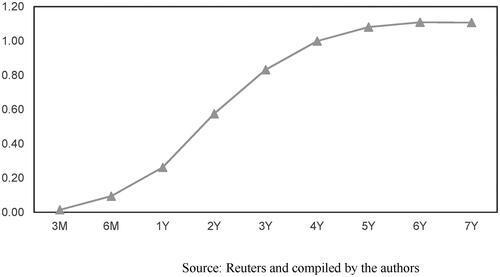
The company’s leasing contract matures in 5 years (September 2026), and therefore, the YTM (IBR) required pertaining to liquid bonds maturing in 5 years is approximately 1.10%. The recovery rate for these bonds is assumed to be 40% (since they are senior, unsecured vanilla bonds), and the average mid-price is 106.81%, paying an average coupon of 2.587%, for that maturity. See Table 7 below for further information on the Reuters curve constituents:

Table 7. Basic materials sector, BB-rated YTM curve bond constituents, 30/09/21.

Issuer name	Coupon (%)	Maturity	Bid	Ask	Swap spread	Asset swap	ISIN
SEALED AIR	4.50	15/09/2023	107.259	107.674	70.5	76.1	XS1247796185
BALL	4.38	15/12/2023	109.331	109.630	56.8	58.6	XS1330978567
BALL	0.88	15/03/2024	101.109	101.488	79.7	77.6	XS2080317832
WIENERBERGER	2.00	02/05/2024	104.672	105.073	57.9	58.7	AT0000A20F93
CROWN EURO	2.63	30/09/2024	104.957	105.412	102.7	103.8	XS1490137418
TITAN GLOBAL	2.38	16/11/2024	103.413	104.413	145.6	144.8	XS1716212243
CROWN EURO	3.38	15/05/2025	107.745	108.007	121.2	125.4	XS1227287221
WIENERBERGER	2.75	04/06/2025	107.516	108.216	86.4	89.7	AT0000A2GLA0
METINVEST	5.63	17/06/2025	105.889	107.389	415.4	420.7	XS2056722734
CROWN EURO	2.88	01/02/2026	106.750	107.121	137.8	141.1	XS1758723883
SYNGENTA FIN	3.38	16/04/2026	109.834	110.162	129.8	135.3	XS2154325489
BALL	1.50	15/03/2027	102.486	104.486	121.2	120.5	XS2080318053
TITAN GLOBAL	2.75	09/07/2027	105.955	106.827	178.3	179.9	XS2199268470
SYNGENTA FIN	1.25	10/09/2027	101.021	101.425	122.9	121.7	XS1199954691
ASHLAND SVC	2.00	30/01/2028	104.183	104.690	142.5	143.3	XS2103218538
VERALLIA	1.63	14/05/2028	103.490	103.966	117.9	118.3	FR0014003G27

Source: compiled by the authors.

Using this information, we are able to calibrate a default-tree similar to the one shown in Table 5, obtaining an implied hazard rate of 2.7365% and with the tree set up for a shift in the recovery rate.

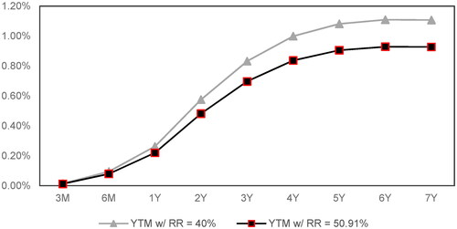
As previously stated, the leased asset (used as collateral) is a machinery-type asset. Based on historical data from Hartmann-Wendels et al. (2014), this asset has a recovery rate of approximately 50.91%. Therefore, all that is required is a shift from 40% to 50.91% to be made in the Recovery Rate used in the tree and, as a result, the new bond price would be 108.25%, meaning a ΔYTM = −0.1789% or −17.89 basis points, thus decreasing from the original YTM (1.10%) to the new lower YTM (0.9211%). This change could hence be applied proportionally to all available, liquid maturities of the standard YTM curve for a given sector and rating in order to make the adjustment required, thereby resulting in a new YTM curve adapted to the required recovery rate. Figure 3 below simulates this shift from the original YTM curve to the new curve adapted to the machinery recovery rate, for all available maturities:

Figure 3. Basic Materials sector, BB standard and shifted YTM curves, 30/09/2021.

Source: Reuters and compiled by the authors

3.5. Comments/Model limitations

Using the framework we have outlined above, we attempt to provide a solution for obtaining an adequate, reliable IBR by using bond market data from companies similar to a lessee, achieving an IBR equal to the shifted YTM given the collateral recovery rate.

In the case of upper investment grade ratings, negative YTMs are currently in place in shorter maturities for several sectors. However, it is worth noting that negative YTMs in leasing contracts are particularly rare, hence a floor at 0% may be set in this regard. Generally speaking, this is not a problem in itself, since an additional liquidity spread is usually attached to this kind of contract, as will be explained below.

The model presents two main limitations (Delgado-Vaquero et al., 2020). The first is related to the liquidity risk attached to any leasing contract, namely the fact that quoted debt is much more liquid than a leasing contract. So, an additional liquidity spread regarding with the nature of the collateral, the contract extension and the collateral expected degree-of-use may be added should be added to both the standard and the adjusted curve⁹.

The second limitation is related to the lack of liquidity or, even, lack of financial products in certain scenarios. There could be situation in which no applicable products can be found and in which further assumptions should be applied.

Last but not least, one further specific limitation to our model should be noted. Certain situations arising from credit events and poorly collateralized assets may mean that the model does not capture the entire actual YTM change. For instance, the change in YTM seen between secured debt and subordinated debt for entities with low credit ratings could not be fully captured by the model because these entities may suffer from incremental spreads required by the market to compensate the “collateral” risk.

4. Empirical Analysis

4.1. Analysis of two specific cases

In order to test our hypothesis and to corroborate our model, we have performed several analyses using quoted bonds. More specifically, we have focused on issuers that maintain quoted bonds with different recovery rates. We have applied our model to the YTM of the standard bond, and subsequently analyzed whether it correctly predicts the YTM of the bond with a different recovery rate.

The bonds contractual data (duration, currency, coupon frequency and type, market conventions, etc.) pertaining to each of the issuers must be similar enough for them to be comparable, thus permitting the main driver behind the differences seen in their YTMs and credit spreads to be their implied LGD (recovery rate), due to the difference in the credit tranche.

In order to illustrate the assessment of our model, we first developed two isolated use cases (which we subsequently extended to a wider sample). The first test was carried out using quoted bonds issued by BBVA (BBVA.MC). We selected three bonds which were highly similar to each other in terms of issuer, currency and duration, but which belonged to different seniority tranches (Table 8).

Table 8. Several outstanding bonds for BBVA, SA, for several seniority tranches, 30/09/21.

Issuer	ISIN	Maturity	Coupon	Currency	Seniority	Issuance rating	Implied recovery rate
BBVA, SA	XS2013745703	21/06/2026	1.000%	EUR	Senior Unsecured	BBB+ (FTC)	40%
BBVA, SA	ES0413211915	22/11/2026	0.875%	EUR	Senior Secured (Covered Bond)	Aa1 (Moody's)	65%
BBVA, SA	XS1562614831	10/02/2027	3.500%	EUR	Subordinated Unsecured	Baa2 (Moody's)	30%

Source: Reuters.

In this case, we have a standard bond (Sr. Unsecured) with an implied market recovery rate of 40%. Furthermore, BBVA has issued other bonds with similar maturity and currency but belonging to the Senior Secured and Subordinated Unsecured tranches, with recovery rates of approximately 65% and 30% respectively, in line with historical data from Moody’s (Tables 1 and 2).

If we use the proposed default-tree model and simulate the impact on the YTM by changing the original recovery rate as per the Sr. Unsecured note by the recoveries for the other tranches, we obtain the results shown in Table 9 below.

Table 9. Several outstanding bonds for BBVA, SA, for several seniority tranches, and model outputs, 30/09/2021.

Issuer	ISIN	Maturity	Coupon	Currency	Seniority	Issuance Rating	Implied Recovery Rate	Market Price	Model Price	Actual YTM	Actual ΔYTM (from Sr. Unsec. Bond)	Model YTM	Model ΔYTM (from Sr. Unsec. Bond)
BBVA, SA	XS2013745703	21/06/2026	1.000%	EUR	Senior Unsecured	BBB+	40%	104.30%	104.30%	0.0795%		0.0795%
BBVA, SA	ES0413211915	22/11/2026	0.875%	EUR	Senior Secured (Covered Bond)	Aa1	65%	105.50%	105.50%	−0.1980%	−0.2775%	−0.1650%	−0.2445%
BBVA, SA	XS1562614831	10/02/2027	3.500%	EUR	Subordinated Unsecured	Baa2	30%	115.71%	115.71%	0.5030%	+0.4235%	+0.4709%	+0.3914%

Source: Reuters and compiled by the authors.

As can be seen in Table 9, we obtain similar results when comparing the actual YTM for any single bond with the YTM obtained when replacing the original Sr. Unsecured bond recovery rate in the default-tree model (40%) by the corresponding recoveries for the covered bond and the subordinated, unsecured note.

This effect can be seen in the case of CaixaBank (CABK.MC), for example. We compared three outstanding bonds with similar contractual details, with seniority constituting the sole notable difference between them (see Table 10).

Table 10. Several outstanding bonds for CaixaBank, for several seniority tranches, 30/09/2021.

Issuer	ISIN	Maturity	Coupon	Currency	Seniority	Issuance Rating	Implied Recovery Rate
CaixaBank	ES0213307053	09/07/2026	0.750%	EUR	Senior Unsecured	A- (FTC)	40%
CaixaBank	XS2013574038	19/06/2026	1.375%	EUR	Senior Non-Preferred	BBB+ (FTC)	35%
CaixaBank	ES0440609339	11/01/2027	1.250%	EUR	Senior Secured (Covered bond)	AAA (FTC)	65%

Source: Reuters.

The results when shifting the recovery rate in the default-tree model from 40% to 35% and 65% achieve a change in the YTM similar to those directly seen in the quoted YTMs (see Table 11).

Table 11. Several outstanding bonds for CaixaBank, for several seniority tranches, and model outputs, 30/09/21.

Issuer	ISIN	Maturity	Coupon	Currency	Seniority	Issuance Rating	Implied Recovery Rate	Market Price	Model Price	Actual YTM	Actual ΔYTM (from Sr. Unsec. Bond)	Model YTM	Model ΔYTM (from Sr. Unsec. Bond)
CaixaBank	ES0213307053	09/07/2026	0.750%	EUR	Senior Unsecured	A-	40%	102.81%	102.81%	0.1290%		0.1235%
CaixaBank	XS2013574038	19/06/2026	1.375%	EUR	Senior Non-Preferred	BBB+	35%	104.83%	104.83%	0.2910%	+0.1620%	0.2539%	+0.1304%
CaixaBank	ES0440609339	11/01/2027	1.250%	EUR	Senior Secured	AAA	65%	107.28%	107.28%	−0.1724%	−0.3014%	−0.1451%	−0.2685%

Source: Reuters and compiled by the authors.

4.2. Sample

In order to assess the robustness of the model along with its predictive power, we undertook the above analysis once again, this time for a sample of outstanding bonds issued in EUR, USD and GBP. We extensively researched Reuters to locate issuers that have issued more than one bond with different estimated recovery rates (belonging to different seniority tranches) but issued in the same currency, with similar duration and paying a similar coupon. In other words, the bonds under analysis would be so similar in nature that the main explanatory variable for the gap between their YTMs would have to be the seniority tranche. This is necessary in order to analyze whether our model correctly predicts the change in YTM when a change in recovery rate occurs.

We constructed a sample with outstanding bonds from the world’s principal bond markets. Table 12A shows the number of bonds initially included in the sample by exchange market. We included only fixed rate bonds, issued by corporates or financial institutions, with maturity dates between 2026 and 2040. For this reason (i.e., the fact that we can only use issuers that have issued more than one bond with different estimated recovery rates), we have analyzed several bond markets with hundreds of potential bonds in order to build a database with sufficient bonds to test model outputs. For the most part, the potential population of quoted bonds is expected to be highly limited and to belong to financial entities. More specifically, using a manual selection process, we obtained 91 bonds issued by 43 issuers (see Annex I, Table 13), all of which complied with the criteria of same issuer, maturity year and different debt seniority (unsecured vs. subordinated/non-preferred/mortgage/secured).

Table 12. Initial sample.

Exchange	Bonds
Deutsche Boerse AG	2,853
Dublin	1,380
Euronext.liffe Paris	771
London	1,264
Luxembourg	1,927
NYSE	3,191
Singapore	596
Vienna Stock Exchange	341
TOTAL	12,323

Source: compiled by the authors.

Table 13. Bonds used for model testing, 30/09/2021.

Bond	Maturity	Seniority	ISIN	Coupon (%)	Mod. Duration
Bayerische Landesbank 2016 1.4% 29/06/29	2029	Senior Unsecured	DE000BLB32E3	1.4	7.3428
Bayerische Landesbank 2018 1 3/4% 17/10/28	2028	Subordinated Unsecured	DE000BLB6TV4	1.75	6.5154
Dekabank Deutsche Girozentrale 2018 1.33% 25/01/30	2030	Senior Unsecured	DE000DK0PDR8	1.33	7.8796
Dekabank Deutsche Girozentrale 2020 1 1/4% 01/04/30	2030	Senior Non-Preferred	DE000DK0T1B2	1.25	8.0626
Dekabank Deutsche Girozentrale 2020 1.1% 25/11/30	2030	Subordinated Unsecured	DE000DK0T2A2	1.1	8.6042
Deutsche Bank AG 2011 4 1/4% 14/09/26	2026	Senior Unsecured	DE000DB7XNA3	4.25	4.5877
Deutsche Bank AG 2016 4.2% 15/06/26	2026	Subordinated Unsecured	DE000DL19S19	4.2	4.209
Aareal Bank AG 2018 0.8% 05/09/28	2028	Mortgage	DE000A2E4CE8	0.8	6.8061
Aareal Bank AG 2019 0.87% 28/06/29	2029	Senior Non-Preferred	DE000A2E4CV2	0.87	7.4798
ABN Amro Bank NV 2016 1% 13/04/31 CBB16	2031	Senior Secured	XS1394791492	1	9.1608
ABN Amro Bank NV 2021 1% 02/06/33 Regulation S	2033	Senior Non-Preferred	XS2348638433	1	10.9892
Altice Financing SA 2021 4 1/4% 15/08/29 Regulation S	2029	Senior Secured	XS2373430425	4.25	6.6425
Altice France Holding 2020 4% 15/02/28 Regulation S	2028	Senior Unsecured	XS2138140798	4	5.5535
Argentum Capital SA 2019 2.1% 19/01/26	2026	Senior Secured	XS1947921075	2.1	4.0979
Argentum Capital SA 2020 1.7% 27/01/27	2027	Senior Unsecured	XS2090803466	1.7	5.0289
Bayerische Landesbank 2016 1/2% 24/03/26	2026	Mortgage	DE000BLB3Z54	0.5	4.4736
Bayerische Landesbank 2017 0.55% 09/08/27	2027	Senior Unsecured	DE000BLB43N1	0.55	3.3615
Banque Nationale de Paris Paribas SA 2016 2 1/4% 11/01/27 Regulation S	2027	Subordinated Unsecured	XS1470601656	2.25	4.9962
Banque Nationale de Paris Paribas SA 2018 1 1/8% 11/06/26 Regulation S	2026	Senior Non-Preferred	XS1748456974	1,125	4.6158
Commerzbank AG 2018 7/8% 06/06/28	2028	Mortgage	DE000CZ40MV5	0.875	6.542
Commerzbank AG 2019 0.85% 15/08/29	2029	Senior Non-Preferred	DE000CZ40N95	0.85	7.6003
Deutsche Bank AG 2015 1 3/4% 09/04/35	2035	Senior Unsecured	DE000DB7XLM2	1.75	11.9416
Deutsche Bank AG 2018 1.405% 04/11/33	2033	Mortgage	DE000DL19T91	1,405	11.165
DZ Bank AG Deutsche 2016 0.67% 18/05/27	2027	Senior Secured	DE000DG4T8R7	0.67	5.5727
DZ Bank AG Deutsche 2017 0.725% 21/06/27	2027	Senior Unsecured	DE000DG4UAZ5	0.725	5.6353
DZ Bank AG Deutsche 2020 1/2% 18/02/27	2027	Subordinated Unsecured	DE000DDA0V15	0.5	5.2993
Elia Transmission 2013 3 1/4% 04/04/28 Regulation S	2028	Senior Unsecured	BE0002432079	3.25	5.9756
Elia Transmission 2014 3% 07/04/29	2029	Unsecured	BE0002466416	3	6.8425
Landesbank Hessen 2016 1.06% 08/11/27	2027	Senior Unsecured	DE000HLB2KP8	1.06	5.8954
Landesbank Hessen 2017 0.997% 30/11/27	2027	Senior Secured	DE000HLB2NE6	0.997	6.0167
Landesbank Hessen 2017 1.745% 20/02/35 Regulation S	2035	Senior Unsecured	XS1567856445	1.745	11.9509
Landesbank Hessen 2018 1 1/4% 19/09/33	2033	Senior Secured	DE000HLB4U71	1.25	11.1228
Landesbank Saar 2015 1 1/4% 23/12/26	2026	Senior Unsecured	DE000SLB5862	1.25	5.0716
Landesbank Saar 2015 1% 15/05/26	2026	Senior Secured	DE000SLB3917	1	4.5692
Landesbank Saar 2017 0.83% 28/09/26	2026	Mortgage	DE000SLB1358	0.83	4.9253
Muenchener Hypothekenbank 2017 5/8% 07/05/27 1762	2027	Mortgage	DE000MHB18J6	0.625	5.5605
Muenchener Hypothekenbank 2019 1/2% 08/06/26	2026	Senior Non-Preferred	DE000MHB61E7	0.5	4.6539
Norddeutsche Landesbank 2013 2.13% 24/04/28	2028	Senior Secured	DE000NLB1LD6	2.13	6.2117
Norddeutsche Landesbank 2014 2 1/2% 23/05/28 1766	2028	Senior Non-Preferred	DE000NLB8CQ2	2.5	6.154
Unicredit Bank AG 2018 1% 29/03/28	2028	Senior Unsecured	DE000HVB29D7	1	6.3414
Unicredit Bank AG 2019 7/8% 11/01/29	2029	Mortgage	DE000HV2ARM0	0.875	7.0988
WCFS und Ifbk Hessen 2016 5/8% 10/06/26	2026	Senior Unsecured	DE000A1R0162	0.625	4.6814
WCFS und Ifbk Hessen 2018 7/8% 14/06/28	2028	Senior Non-Preferred	DE000A2DAF36	0.875	6.5746
BARCLAYS PLC 2016 4 3/8% 12/01/26 S	2026	Senior Unsecured	US06738EAN58	4.375	5.2162
BARCLAYS PLC 2016 5.2% 12/05/26 S	2026	Subordinated Unsecured	US06738EAP07	5.2	5.3163
FORD MOTOR COMPANY 1992 9.95% 15/02/32 P02/95	2032	Unsecured	US345370BH27	9.95	7.7727
FORD MOTOR COMPANY 1998 8.9% 15/01/32 S	2032	Senior Unsecured	US345370BV11	8.9	7.8014
HCA INCORPORATED 2016 5 1/4% 15/06/26 S	2026	First Lien	US404119BT57	5.25	5.4084
HCA INCORPORATED 2018 5 3/8% 01/09/26 S	2026	Senior Unsecured	US404121AH82	5.375	5.453
MORGAN STANLEY 2014 4.35% 08/09/26 F	2026	Subordinated Unsecured	US6174467Y92	4.35	5.6565
MORGAN STANLEY 2016 3 7/8% 27/01/26 F	2026	Senior Unsecured	US61746BDZ67	3.875	5.326
STATE STREET CORP. 2020 2.4% 24/01/30 S	2030	Senior Unsecured	US857477BG73	2.4	8.7868
STATE STREET CORP. 2021 2.2% 03/03/31 S	2031	Senior Subordinated Unsecured	US857477BP72	2.2	8.9012
WELLS FARGO & CO 2005 5 1/2% 01/08/35 S	2035	Subordinated Unsecured	US929903AM44	5.5	11.0967
WELLS FARGO & CO 2005 5 3/8% 07/02/35 S	2035	Senior Unsecured	US949746JM44	5.375	10.9647
ALLGEMEINE SPARK. 2015 1.13% 16/02/27 2	2027	Senior Secured	AT000B101076	1.13	6.7712
ALLGEMEINE SPARK. 2017 1.4% 05/07/27 4	2027	Senior Unsecured	AT000B101274	1.4	6.9756
BANK FUER TIROL 2017 1.72% 10/03/27 7	2027	Senior Unsecured	AT0000A1U834	1.72	6.7522
BANK FUER TIROL 2018 1.325% 22/03/28 3	2028	Senior Secured	AT0000A20BV7	1.325	7.5126
BANK OF AM CORP 2008 7% 31/07/28 REG.S	2028	Senior Unsecured	XS0379947236	7	6.7953
BANK OF AM CORP 2008 8 1/8% 02/06/28 REG.S	2028	Subordinated	XS0365909125	8.125	6.3112
BQ.FEDV.DCM.SA 2017 1.43% 05/04/29 REG.S	2029	Senior Unsecured	XS1591784639	1.43	8.5542
BQ.FEDV.DCM.SA 2019 1 7/8% 18/06/29	2029	Subordinated	FR0013425162	1.875	8.4953
CANADA HSG.TST.NO.1 2021 1.4% 15/03/31 97	2031	Second Lien	CA13509PHS52	1.4	9.246
CANADA HSG.TST.NO.1 2021 1.6% 15/12/31 101	2031	Senior Unsecured	CA13509PHW64	1.6	9.12
CMWL.BK.OF AUS. 2010 4.3% 13/08/32 REG.S	2032	Senior Unsecured	XS0532303186	4.3	9.6195
CMWL.BK.OF AUS. 2012 3.994% 13/02/30 REG.S	2030	Senior Secured	XS0745915826	3.994	8.6623
COMPAGNIE DE FNCMT. 2012 2.915% 14/12/32 580	2032	Secured	FR0011370378	2.915	11.1328
COMPAGNIE DE FNCMT. 2013 3.05% 22/08/33	2033	Senior Secured	FR0011553684	3.05	11.4642
COOPERATIEVE RABO. 2016 1.43% 01/09/36 REG.S	2036	Senior Unsecured	XS1484005985	1.43	14.6276
COOPERATIEVE RABO. 2018 1.595% 08/03/38 REG.S	2038	Mortgage	XS1785456713	1.595	15.7994
CREDIT AGRICOLE S A 2015 2.129% 10/09/27 REG.S	2027	Senior Unsecured	XS1288342493	2.129	6.9997
CREDIT AGRICOLE SA 2016 2.3% 24/10/26 Q	2026	Subordinated	FR0013192762	2.3	6.2032
CTRY.GDN.HDG.CTD. 2020 4.2% 06/02/26 REG.S	2026	Senior Unsecured	XS2210960022	4.2	5.91
CTRY.GDN.HDG.CTD. 2020 5 1/8% 14/01/27 REG.S	2027	First Lien	XS2100725949	5.125	5.7579
DEUTSCHE APOTH.UND 2016 0.825% 17/06/26 REG.S	2026	Senior Unsecured	XS1434566250	0.825	6.1414
DEUTSCHE APOTH.UND 2017 3/4% 05/10/27 REG.S	2027	Mortgage	XS1693853944	0.75	7.4473
DWR CYMRU FNG.UK 2020 1 3/8% 31/03/33 REG.S	2033	Senior Secured	XS2115092442	1.375	12.164
DWR CYMRU FNG.UK 2021 2 3/8% 31/03/34 REG.S	2034	Subordinated Secured	XS2328412064	2.375	12.95
ERSTE GROUP BANK AG 2010 4.41% 21/04/30 932	2030	Mortgage	AT000B008248	4.41	7.7974
ERSTE GROUP BANK AG 2014 4.46% 20/12/29 1329	2029	Subordinated	AT0000A18991	4.46	8.2058
LA BANQUE PTLE.SA 2016 2 1/4% 05/10/28	2028	Subordinated	FR0013207354	2.25	7.7892
LA BANQUE PTLE.SA 2018 2% 13/07/28 61	2028	Senior Non-Preferred	FR0013349099	2	7.7412
LANDESBANK BWTG. 2001 5.7% 28/02/31 226	2031	Senior Non-Preferred	XS0125912336	5.7	8.6898
LANDESBANK BWTG. 2001 6.19% 30/06/31 236	2031	Subordinated	XS0131928391	6.19	8.7209
LLOYDS BANK PLC 2015 1.326% 23/04/30 REG.S	2030	Senior Unsecured	XS1220089590	1.326	9.3407
LLOYDS BANK PLC 2016 1.35% 01/02/31 REG.S	2031	Senior Secured	XS1354465566	1.35	10.2776
NAT AUS BK LTD 2015 7/8% 19/02/27 REG.S	2027	Senior Secured	XS1191309720	0.875	6.7783
NAT AUS BK LTD 2016 0.655% 15/03/27 REG.S	2027	Senior Unsecured	XS1490954978	0.655	6.8853
RAIFF.LB.TIROL AG 2016 1.175% 20/07/26	2026	Senior Unsecured	AT0000A1MBY1	1.175	6.1406
RAIFF.LB.TIROL AG 2017 0.95% 15/11/27	2027	Senior Secured	AT0000A1Z080	0.95	6.75

Source: Reuters and compiled by the authors.

4.3. Model performance assessment

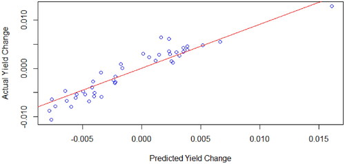
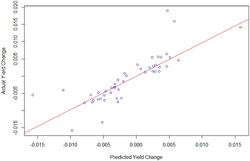
Once the theoretical YTM change was computed for each pair of bonds following the tree model explained above (Section 3), we performed a regression analysis on the model output (i.e., the theoretical, predicted ΔYTM vs. the actual ΔYTM currently seen in the market for each pair of bonds) as of same banking day (30/09/2021). Figure 4 below contains a summary of the main results for an ordinary-least squares regression.

Figure 4. OLS regression, Predicted ΔYTM vs Actual ΔYTM, 30/09/2021.

Source: compiled by the authors

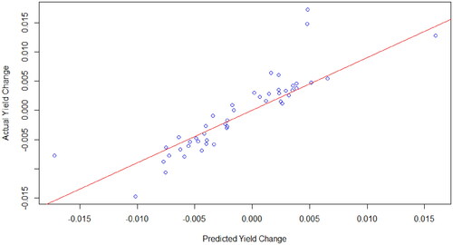
The statistical outputs reflect a robust goodness-of-fit of the predicted ΔYTM compared to the actual one. For an OLS linear regression with the modeled YTM as the explanatory variable, R² reaches 0.7491, taking into account that there are certain outliers identified in the series which penalize the final outcome. The estimator is 0.90011, being significative with a p-value of 2.08e-15 and t-test value of 11.72 for 46 degrees of freedom.

It should also be noted that no evidence of heteroskedasticity in the Breusch-Pagan test (assuming linear relationship) has been identified. However, full normality in residuals cannot be assumed as per the Jarque-Bera test output and Q-Q plot, due to the four outliers already identified in the regression outcome (Figure 5).

Figure 5. Normal Q-Q Plot, Predicted ΔYTM vs Actual ΔYTM, 30/09/2021.

Source: compiled by the authors

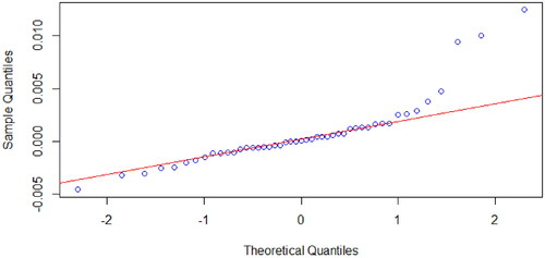
The abovementioned outliers within the bond sample are issuances from Ford, Deutsche Bank, Altice Financing and Erste Group. Some of these issuances have in common a low rating score (speculative grade), with particular emphasis on the subordinated bonds from Deutsche Bank and Erste Group. The difference between the predicted ΔYTMs and the actual ones seen between the pair of bonds when one bond is located in the subordinated tranche is relatively high (more than 100 bp), considering that the model does not capture some issuance-specific situations. This means that while the model accurately predicts the expected direction and amount of the ΔYTM arising from a change in the expected Recovery Rate, in certain specific cases when the change in the tranche level for issuances from the same entity is relatively high (e.g., when the pair of bonds is composed by a secured note and a subordinated unsecured bond), then the market requires an additional risk premium to the issuance in the lower tranche.

If we eliminate the outliers from the sample, we obtain the regression output shown below in Figure 6.

Figure 6. OLS regression without outliers, Predicted ΔYTM vs Actual ΔYTM, 30/09/2021.

Source: compiled by the authors

The goodness-of-fit of the predicted ΔYTM increases considerably, with R² reaching 0.8929. For an OLS linear regression with the modeled YTM as the explanatory variable, the estimator is 0.90685, with the t-test value equal to 18.71 and p-value < 2e-16.

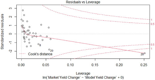
It is now possible to assume the normality in residuals with a Jarque-Bera test output of 1.1749 and a p-value = 0.5557, with the following Q-Q plot and Cook’s distance (Figures 7 and 8).

Figure 7. Normal Q-Q Plot for regression residuals w/out outliers, Predicted ΔYTM vs Actual ΔYTM, 30/09/2021.

Source: compiled by the authors

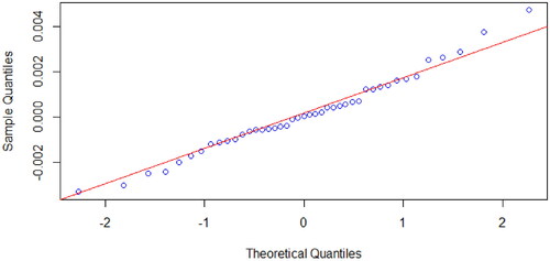
Figure 8. Cook’s distance for regression residuals w/out outliers, Predicted ΔYTM vs Actual ΔYTM, 30/09/2021.

Source: compiled by the authors

Although we have assessed the model robustness for the widest possible population as per our market data base, we also need to assess the model’s predictive power for additional random cases and over different sample sizes, using subsets of the current population in order to predict out-of-sample ΔYTMs.

4.4. Out-of-sample model testing and training

We have already seen that the model replicates the actual YTM change seen in the bond sample for a range of different shifts in the recovery rate to a high degree of confidence. However, we also tested model performance and predictive power by carrying out out-of-sample testing techniques, i.e., cross-validation or resampling methods.

The fundamental principle behind these cross-validation techniques consisted of dividing the data into two sets:

• The training set: used to train (i.e., build) the model.

• The testing set (or validation set): used to test (i.e., validate) the model by estimating the prediction error on the ΔYTM with a sample of the entire bond population used initially.

We have used three main methods for cross-validating the model performance and to assess its predictive power:

1. Leave One Out - Cross Validation: LOOCV

2. Bootstrapping

3. Repeated K-Folds

The main outputs to be analyzed from these methods are as follows:

• The R-squared (R²) as used above, representing the squared correlation between the observed outcome values and the values predicted by the model. The higher the adjusted R², the better the model.

• Root Mean Squared Error (RMSE) which measures the average prediction error made by the model in predicting the outcome for an observation. That is, the average difference between the observed known outcome values and the values predicted by the model. The lower the RMSE, the better the model.

• Mean Absolute Error (MAE) which is an alternative to the RMSE that is less sensitive to outliers. It corresponds to the average absolute difference between observed and predicted outcomes. The lower the MAE, the better the model.

Hence, regarding the outputs of model estimation power:

• 1. LOOCV: we have used it to split the sample into two sections, one of n-1 data points which is used to reproduce a regression for predicting the value of the remaining data points, for each of which a regression of n-1 is calibrated. The output averages are the following:

  • RMSE: 0.00346

  • R²: 0.71182

  • MAE: 0.00221

    Excluding the abovementioned outliers, the values are as follows:

  • RMSE: 0.00184

  • R²: 0.87102

  • MAE: 0.00138

• 2. Bootstrapping: this method randomly selects a sample of n observations from the original data set. This subset is then used to evaluate the model. In this case, the sampling is performed with replacement, which means that the same observation can occur more than once in the bootstrap data set. This provides the advantage of having a large number of potential subsets to simulate data samples. We have simulated 1,000 scenarios with the following output averages:

  • RMSE: 0.00345

  • R²: 0.80007

  • MAE: 0.00231

  • In Figure 9, we can see two outliers and excluding them we obtain better output averages and a fitting of residuals (Figure 10): RMSE: 0.00186

    Figure 9. Residuals fitting for Bootstrap resampling on Predicted ΔYTM, 30/09/2021.

    Source: compiled by the authors

    

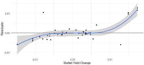
    Figure 10. Residuals fitting for Bootstrap resampling on Predicted ΔYTM, without outliers, 30/09/2021.

    Source: compiled by the authors

    

  • R²: 0.89716

  • MAE: 0.00142

• 3. Repeated K-folds: this method divides the data into k buckets of almost equal size. Of these k folds, one is used as a validation set while the others are involved in calibrating the regression. In this regard, we have implemented a simulation of 1,000 regression folds so as to be able to generate sufficient prediction scenarios, including the outliers within the initial sample, in order to confirm whether the model’s predictive power is robust and does cover the standard relationship between YTM level and the estimated Recovery Rate for random samples. This method can be considered less unbiased than the above since it uses random data for both regression subsamples, including thousands of combinations of training and validation data sets.

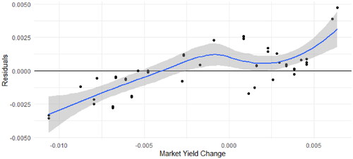
   For a K-fold implementation with the sample divided into 10 buckets, the outputs and are as follows and the fitting of residuals can be sawn in Figure 11 and 12 (no outliers):

  Figure 11. Residuals fitting for Repeated K-Folds on Predicted ΔYTM, 30/09/2021.

  Source: compiled by the authors

  

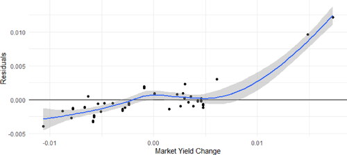
  Figure 12. Residuals fitting for Repeated K-Folds on Predicted ΔYTM, without outliers, 30/09/2021.

  Source: compiled by the authors

  

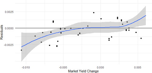
•  • RMSE: 0.00296

•  • R²: 0.9041

•  • MAE: 0.00221

  Excluding the outliers, the values are:

•  • RMSE: 0.00170

•  • R²: 0.93541

•  • MAE: 0.00138

Summarizing the outcomes, we validate our model under three different cross-validating techniques (LOOCV, bootstrapping and repeated K-folds). In the three tests, we obtain RMSEs and MAEs close to zero and high R² (above 90% if excluding outliers). These results confirm to us the performance of the model proposed and its predictive power.

4.5. Testing the model in a pre-pandemic scenario

In order to test the model performance against a different macroeconomic background, and given the fact that the COVID-19 pandemic deeply affected the credit quality of almost every single company worldwide, we have again performed the previous analyses for a banking date of 20/03/2020 for the same bond population. Figure 13 below shows the OLS output for this scenario.

Figure 13. OLS regression, Predicted ΔYTM vs Actual ΔYTM, 20/03/2020.

Source: compiled by the authors

The statistical outputs reflect a robust goodness-of-fit of the predicted ΔYTM similar to that seen at 30/09/2021. Also, R² is relatively strong (0.7003), albeit lower than that obtained for 30/09/2021.

RMSE and MAE related to out-of-sample analysis are also similar to those computed for 30/09/2021 for each of the LOOCV, Bootstrap and Repeated K-folds methods.

5. Conclusions

IFRS 16 introduce a capitalization model which is to be applied by the lessee in the majority of lease transactions. The most widely used rate for discounting future lease payments by entities is the IBR, which must consider the collateral that the leased asset represents for the lessor. A new model is proposed for estimating the IBR. More precisely, we propose a model for adjusting a standard IBR in order to reflect the correct LGD associated with the leased asset.

Our model is based on adjusting the unsecured bond YTM to a YTM applicable to a recovery rate other than 40% (depending on the leased asset’s LGD).The adjustment consists of the percentage change on the YTM assumed for the lessee when a change in the recovery rate occurs. This percentage change is applied to the standard IBR.

The model may be easily implemented by entities that need to maintain several discounting curves depending on the leased asset (and that have different maturity rates). The underlying method is based on a standard cash-flow valuation model relying on the recovery rate for all potential default scenarios.

Following an empirical analysis using 97 quoted bonds and testing the model under cross-validation techniques, we conclude that the following hypothesis can be assumed: our model reflects the expected YTM change in a fixed coupon note due to a change in the recovery rate. The robustness demonstrated by the model’s outputs appears to be sufficient to be applied in most cases. Nonetheless, as previously mentioned, there may be specific situations where the predicted ΔYTM does not reflect the actual ΔYTM.

We further conclude that our model appears sufficiently robust to be used for leasing contracts for which the IBR must be adapted depending on the collateral (leased asset) recovery rate. As previously stated, apart from the lessee credit rating or the collateral quality, additional factors may also influence the IBR, but the basis for the expected change in the IBR can be predicted with this model (assuming the availability of sufficient financial data as per the example set out in Section 3.4).

The model also has certain limitations that should be considered. It is built upon the availability of credit market information, which on occasion is not sufficient for certain type of issuers or sectors. The fact that estimated recovery rates for a given collateral or security may change over time should also be considered, implying the model assumptions and recovery levels need to be revisited frequently. Moreover, it should be noted that several risk factors are not entirely covered by the model (e.g., inherent credit risk, sovereign risk, currency risk); hence, the chosen reference data and market information may contain sample entries that might distort the outcome. Therefore, the relevancy of using market data and securities as similar as possible to the leasing contract under analysis is fundamental.

Disclosure statement

The authors report there are no competing interests to declare.

Notes

1 Except for the corresponding accruals or prepayments.

2 Not for lessors. Lessors still must classify leases as operating or finance leases.

3 Short term leases and leases of low value assets. IFRS 16 paragraph 5.

4 IFRIC: IFRS Interpretations Committee.

5 LGD = 1 – Recovery Rate.

6 Information obtained from their 2019 financial statements.

7 YTM: Yield to Maturity.

8 EBA: European Banking Authority.

9 Nevertheless, is true that IFRS 16 does not explicitly require a liquidity adjustment if the IBR is obtained from a quoted instrument.

Annex I

References

- Akguen, A., & Vanini, P. (2007). Loan pricing: Thinking collateral. Available at SSRN: https://ssrn.com/abstract=963887 or https://doi.org/10.2139/ssrn.963887
- Ando, T. (2014). Bayesian corporate bond pricing and credit default swap premium models for deriving default probabilities and recovery rates. Journal of the Operational Research Society, 65(3), 454–465. https://doi.org/10.1057/jors.2013.16
- Bastos, J. A. (2010). Forecasting bank loans loss-given-default. Journal of Banking & Finance, 34(10), 2510–2517. https://doi.org/10.1016/j.jbankfin.2010.04.011
- Beattie, V., Edwards, K., & Goodacre, A. (1998). The impact of constructive operating lease capitalisation on key accounting ratios. Accounting and Business Research, 28(4), 233–254. https://doi.org/10.1080/00014788.1998.9728913
- Bellucci, A., Borisov, A., Giombini, G., & Zazzaro, A. (2021). Estimating the relationship between collateral and interest rate: A comparison of methods. Finance Research Letters, 43, 101962. https://doi.org/10.1016/j.frl.2021.101962
- Benmelech, E., & Bergman, N. K. (2009). Collateral pricing. Journal of Financial Economics, 91(3), 339–360. https://doi.org/10.1016/j.jfineco.2008.03.003
- Benmelech, E., & Bergman, N. K. (2011). Bankruptcy and the collateral channel. The Journal of Finance, 66(2), 337–378. https://doi.org/10.1111/j.1540-6261.2010.01636.x
- Bennett, B. K., & Bradbury, M. E. (2003). Capitalizing non-cancellable operating leases. Journal of International Financial Management and Accounting, 14(2), 101–114. https://doi.org/10.1111/1467-646X.00091
- Berger, A. N., & Udell, G. F. (1990). Collateral, loan quality and bank risk. Journal of Monetary Economics, 25(1), 21–42. https://doi.org/10.1016/0304-3932(90)90042-3
- Besanko, D., & Thakor, A. V. (1987). Competitive equilibrium in the credit market under asymmetric information. Journal of Economic Theory, 42(1), 167–182. https://doi.org/10.1016/0022-0531(87)90108-6
- Blazy, R., & Weill, L. (2013). Why do banks ask for collateral in SME lending? Applied Financial Economics, 23(13), 1109–1122. https://doi.org/10.1080/09603107.2013.795272
- Blum, V., & Thérond, P. E. (2019). Discount rates in IFRS: How practitioners depart the IFRS maze. Research Report – Autorité des Normes Comptables. Availabe at: https://hal.archives-ouvertes.fr/hal-01992506/file/DISCOUNT-RATES-IN-ACCOUNTING-from-theories-to-%20practices_Blum.pdf
- Bo, B. (2020). Globally consistent creditor protection, reallocation, and productivity. LawFin Working Paper No. 6, Available at SSRN: https://ssrn.com/abstract=3720573 or https://doi.org/10.2139/ssrn.3720573
- Carlin, T. M., & Finch, N. (2009). Discount rates in disarray: Evidence on flawed goodwill impairment testing. Australian Accounting Review, 19(4), 326–402. https://doi.org/10.1111/j.1835-2561.2009.00069.x
- Carlin, T. M., & Finch, N. (2010). Commentary: Some further evidence on discount rate selection in the context of goodwill impairment testing. Australian Accounting Review, 20(4), 400–402. https://doi.org/10.1111/j.1835-2561.2010.00111.x
- Cerqueiro, G., Ongena, S., & Roszbach, K. (2016). Collateralization, bank loan rates, and monitoring. The Journal of Finance, 71(3), 1295–1322. https://doi.org/10.1111/jofi.12214
- Chan, Y. S., & Kanatas, G. (1985). Asymmetric valuations and the role of collateral in loan agreements. Journal of Money, Credit and Banking, 17(1), 84–95. https://doi.org/10.2307/1992508
- Chiang, S., & Tsai, M. (2010). Pricing a defaultable bond with a stochastic recovery rate. Quantitative Finance, 10(1), 49–58. https://doi.org/10.1080/14697680902835725
- Delgado-Vaquero, D., & Morales-Díaz, J. (2018). Estimating a credit rating for accounting purposes: A quantitative approach. Estudios de Economía Aplicada, 36(2), 459–488. https://doi.org/10.25115/eea.v36i2.2539
- Delgado-Vaquero, D., Morales-Díaz, J., & Zamora-Ramírez, C. (2020). IFRS 9 expected loss: A model proposal for estimating the probability of default for non-rated companies. Revista de Contabilidad, 23(2), 180–196. https://doi.org/10.6018/rcsar.370951
- Deloitte. (2018). A guide to the incremental borrowing rate. Available at: https://www2.deloitte.com/content/dam/Deloitte/ch/Documents/audit/ch-en-audit-discount-rate-publication.pdf
- Duo, Y., & Meder, A. A. (2020). Observed risk and loss reduction effects of collateral on loan pricing. Available at: https://web.archive.org/web/20201106062804id_/https://s3.eu-central-1.amazonaws.com/ng-submission-additional-files/AAA-AM-2020/5f0c7d3058e581e69b05d0c6/files/Duo-Meder-July-2020.pdf
- Duffie, D., & Singleton, K. J. (1999). Modeling term structures of defaultable bonds. Review of Financial Studies, 12(4), 687–720. https://doi.org/10.1093/rfs/12.4.687
- Duke, J. C., Hsieh, S. J., & Su, Y. (2009). Operating and synthetic leases: Exploiting financial benefits in the post-Enron era. Advances in Accounting, 25(1), 28–39. https://doi.org/10.1016/j.adiac.2009.03.001
- Durocher, S. (2008). Canadian evidence on the constructive capitalization of operating leases. Accounting Perspectives, 7(3), 227–256. https://doi.org/10.1506/ap.7.3.2
- EBA. (2017). Guidelines on PD estimation, LGD estimation and the treatment of defaulted exposures. Available at: https://www.eba.europa.eu/sites/default/documents/files/documents/10180/2033363/6b062012-45d6-4655-af04-801d26493ed0/Guidelines%20on%20PD%20and%20LGD%20estimation%20%28EBA-GL-2017-16%29.pdf?retry=1
- Ely, K. M. (1995). Operating lease accounting and the market’s assessment of equity risk. Journal of Accounting Research, 33(2), 397–415. https://doi.org/10.2307/2491495
- Fitó, M. A., Moya, S., & Orgaz, N. (2013). Considering the effects of operating lease capitalization on key financial ratios. Spanish Journal of Finance and Accounting / Revista Española de Financiación y Contabilidad, 42(159), 341–369. https://doi.org/10.1080/02102412.2013.10779750
- Frontczak, R., & Rostek, S. (2015). Modeling loss given default with stochastic collateral. Economic Modelling, 44(C), 162–170. https://doi.org/10.1016/j.econmod.2014.10.006
- Fülbier, U. R., Silva, J. L., & Pferdehirt, H. M. (2008). Impact of lease capitalization on financial ratios of listed German companies. Schmalenbach Business Review, 60(2), 122–145. https://doi.org/10.1007/BF03396762
- Giner, B., Merello, P., & Pardo, F. (2019). Assessing the impact of operating lease capitalization with dynamic Monte Carlo simulation. Journal of Business Research, 101, 836–845. https://doi.org/10.1016/j.jbusres.2018.11.049
- Gonas, J. S., Highfield, M. J., & Mullineaux, D. J. (2004). When are commercial loans secured? Financial Review, 39(1), 79–99. https://doi.org/10.1111/j.0732-8516.2004.00068.x
- Goodacre, A. (2003). Assessing the potential impact of lease accounting reform: A review of the empirical evidence. Journal of Property Research, 20(1), 49–66. https://doi.org/10.1080/0959991032000051962
- Grossman, A. M., & Grossman, S. D. (2010). Capitalizing lease payments. CPA Journal, 80(5), 6–11.
- Hartmann-Wendels, T., Miller, P., & Töws, E. (2014). Loss given default for leasing: Parametric and nonparametric estimations. Journal of Banking & Finance, 40, 364–375. https://doi.org/10.1016/j.jbankfin.2013.12.006
- Husmann, S., & Schmidt, M. (2008). The discount rate: A note on IAS 36. Accounting in Europe, 5(1), 49–62. https://doi.org/10.1080/17449480802088762
- IFRIC. (2019). IFRIC Update June 2019. Available at: https://www.ifrs.org/news-and-events/updates/ifric-updates/june-2019/#3
- IFRS. (2019). IFRS staff paper: IFRS Interpretations Committee Meeting September 2029. Available at: https://cdn.ifrs.org/-/media/feature/meetings/2019/september/ifric/ap8-lessees-incremental-borrowing-rate-ifrs-16.pdf
- Imhoff, E. a., Jr., & Lipe, R. C. (1991). Operating leases: Impact of constructive capitalization. Accounting Horizons, 5(1), 51–63.
- Imhoff, E. a., Jr., & Lipe, R. C. (1997). Operating leases: Income effects of constructive capitalization. Accounting Horizons, 11(2), 12–32.
- Jarrow, R., & Turnbull, S. (1995). Pricing derivatives on financial securities subject to credit risk. The Journal of Finance, 50(1), 53–85. https://doi.org/10.1111/j.1540-6261.1995.tb05167.x
- KPMG. (2017). Leases discount rates. What’s the correct rate? Available at: https://home.kpmg.com/content/dam/kpmg/xx/pdf/2017/09/leases-discount-rate.pdf
- Lara-Rubio, J., Blanco-Oliver, A., & Pino-Mejías, R. (2017). Promoting entrepreneurship at the base of the social pyramid via pricing systems: A case study. Intelligent Systems in Accounting, Finance and Management, 24(1), 12–28. https://doi.org/10.1002/isaf.1400
- Luck, S., & Santos, J. A. C. (2022). The valuation of collateral in bank lending (2021 version). Risk Management & Analysis in Financial Institutions eJournal. https://doi.org/10.2139/ssrn.3467316
- Matias, A. P., & Dias, F. (2015). Collateral and relationship lending in loan pricing: Evidence from UK SMEs. WSEAS Transactions on Business and Economics, 12, 21–35.
- Miao, H., Ramchander, S., & Wang, T. (2014). The response of bond prices to insurer ratings changes. The Geneva Papers on Risk and Insurance - Issues and Practice, 39(2), 389–413. https://doi.org/10.1057/gpp.2013.21
- Michelon, G., Paananen, M., & Schneider, T. (2020). Black box accounting: Discounting and disclosure practices of decommissioning liabilities. ICAS. Available at: https://www.icas.com/__data/assets/pdf_file/0005/559733/Black-box-accounting-discounting-and-decomissioning-08-10-20.pdf
- Miller, P., & Töws, E. (2018). Loss given default adjusted workout processes for leases. Journal of Banking & Finance, 91, 189–201. https://doi.org/10.1016/j.jbankfin.2017.01.020
- Moody’s. (2018). Annual default study: Corporate default and recovery rates, 1920–2017. Available at: https://www.moodys.com/Pages/Default-and-Recovery-Analytics.aspx?stop_mobi=yes
- Morales-Díaz, J., & Zamora-Ramírez, C. (2018a). IFRS 16 (leases) implementation: Impact of entities’ decisions on financial statements. AESTIMATIO, the IEB International Journal of Finance, 17, 60–97. https://doi.org/10.5605/IEB.17.4
- Morales-Díaz, J., & Zamora-Ramírez, C. (2018b). Impact of IFRS 16 on key financial ratios: A new methodological approach. Accounting in Europe, 15(1), 105–133. https://doi.org/10.1080/17449480.2018.1433307
- Morales-Díaz, J., Villacorta-Hernández, M. A., & Voicila, F. I. (2019). Lease accounting: An inquiry into the origins of the capitalization model. De Computis - Revista Española de Historia de la Contabilidad, 16(2), 160–187. https://doi.org/10.26784/issn.1886-1881.v16i2.357
- Mulford, C., & Gram, M. (2007). The effects of lease capitalization on various financial measures: An analysis of the retail industry. Journal of Applied Research in Accounting and Finance, 2(2), 3–13.
- Ou, S., Chiu, D., & Metz, A. (2016). Annual default study: Corporate default and recovery rates, 1920–2015. Moodyśs investor service, (May), 1–76. Retrieved from https://www.moodys.com/researchdocumentcontentpage.aspx?docid=PBC_1018455
- Pardo, F., & Giner, B. (2017). Operating lease decision and the impact of capitalization in a bank-oriented country. Applied Economics, 49(19), 1886–1900. https://doi.org/10.1080/00036846.2016.1229416
- Qi, M., & Zhao, X. (2011). Comparison of modeling methods for loss given default. Journal of Banking & Finance, 35(11), 2842–2855. https://doi.org/10.1016/j.jbankfin.2011.03.011
- Schneider, T., Michelon, G., & Maier, M. (2017). Environmental liabilities and diversity in practice under international financial reporting standards. Accounting, Auditing & Accountability Journal, 30(2), 378–403. https://doi.org/10.1108/AAAJ-01-2014-1585
- Schonbucher, P. J. (2003). Credit derivatives pricing models: Models, pricing and implementation. Wiley Finance.
- Silaghi, F., Martin-Oliver, A., & Sewaid, A. (2020). The CDS market reaction to loan renegotiation announcements. Available at SSRN: https://ssrn.com/abstract=3546561 or https://doi.org/10.2139/ssrn.3546561
- Singh, A. (2012). Proposed lease accounting changes: Implications for the restaurant and retail industries. Journal of Hospitality & Tourism Research, 36(3), 335–365. https://doi.org/10.1177/1096348010388659
- Spuchľakova, E., & Cug, J. (2015). Credit risk and LGD modelling. Procedia Economics and Finance, 23, 439–444. https://doi.org/10.1016/S2212-5671(15)00379-2
- Uhrig-Homburg, M., & Kempf, A. (2000). Liquidity and its impact on bond prices. Schmalenbach Business Review, 52, 26–44. Available at SSRN: https://ssrn.com/abstract=311025 or https://doi.org/10.2139/ssrn.311025
- Wong, K., & Joshi, M. (2015). The impact of lease capitalisation on financial statements and key ratios: Evidence from Australia. Australasian Accounting, Business and Finance Journal, 9(3), 27–44. https://doi.org/10.14453/aabfj.v9i3.3
- Yashkir, O., & Yashkir, Y. (2013). Loss given default modelling: Comparative analysis. Journal of Risk Model Validation, 7(1), 1–28. Available at: https://mpra.ub.uni-muenchen.de/46147/1/MPRA_paper_46147.pdf