Modelling returns volatility: mixed-frequency model based on momentum of predictability

Abstract

The estimation and prediction of financial asset volatility are important in terms of theoretical and practical applications. Considering that low-frequency and high-frequency information plays an important role in volatility prediction, this article proposes a mixed-frequency model based on the momentum of predictability (MF-MoP). To illustrate the advantages of the proposed model, comparative research is conducted on the prediction accuracy of volatility among the GARCH model, the Realized GARCH model and the MF-MoP model, by the loss function and MCS test. The empirical results show that the MF-MoP model has higher prediction accuracy than the other two models; especially based on skewed-t distribution, the MF-MoP significantly outperforms the competing models. Moreover, the MF-MoP model can improve the forecasting of volatility, regardless of different look-back periods (including 1, 3, 6 and 9 days), different data (including the CSI 300 index, the N225 index and the KS11 index), and realized measures (including RV, RRV and MedRV), indicating that the model is robust.

Keywords:

• Mixed-frequency
• prediction
• loss function
• MCS test
• realized measures

JEL CODES:

• G17
• C22
• C52
• C53

1. Introduction

Financial asset volatility plays a crucial role in risk management, derivative asset pricing, portfolio selection and other related fields. In risk management, financial institutions often use the volatility of return to measure risk. In asset pricing, the option price depends on a precise forecast of the underlying asset volatility (Hongwiengjan & Thongtha, 2021). In optimal management of asset portfolios, volatility is often used as an indicator to construct optimal portfolio weights. However, volatility usually refers to the variance of asset returns, which measures the change in the degree of returns, and cannot be directly observed. The data on volatility can be extracted only from the evolution process or distribution characteristics of return series, which is also a major challenge in volatility modelling. Therefore, the purpose of this article is to build a model that can describe the characteristics of volatility, while estimating and predicting volatility. Numerous studies link stock returns at a low-frequency (e.g., monthly or daily information) with high-frequency data based on intraday information to study stock volatility and demonstrate superior forecasting abilities for volatility (see, e.g., Andreou, 2016; Zhang et al., 2019; Wang et al., 2020; Yu & Huang, 2021; Ma et al., 2021). Therefore, it is important to thoroughly utilise the rich information available for high-frequency data and macro low-frequency to accurately depict the stock market volatility and explore the operating mechanism of the stock market. This can aid in optimising portfolio strategy, alleviating losses, and avoiding risks.

Considering that low-frequency and high-frequency information plays an important role in volatility prediction, this article proposes a mixed-frequency model based on the momentum of predictability (MF-MoP). The proposed model combines the GARCH model based on low-frequency data, and the Realized GARCH model based on highfrequency data, using the momentum of predictability. This model also uses the information on low-frequency and high-frequency data to construct the long-term volatility of stock market using the relative performances of GARCH and Realized GARCH models. Furthermore, financial returns often have peak fat-tail characteristics. Considering that the model is based on the assumption that normal innovation cannot capture the skewness and leptokurtosis of typical asset returns, the skewed-t distribution accurately captures the typical characteristics of financial data (see, e.g., Liu et al., 2015; Tian & Hamori, 2015). We introduce the skewed-t distribution into the MF-MoP model to predict out-of-sample volatility. In empirical analysis, we adopt the MF-MoP model to the CSI 300 index (CSI300). Our empirical results indicate the MF-MoP model improves the effect on volatility forecasts. In particular, the MF-MoP model based on skewed-t distribution significantly outperforms the competing models. In the robustness test, N225 and KS11 indexes are used to verify the robustness of the MF-MoP model. Additionally, we also study the effects of different realized measures on the model results. The abovementioned robustness tests support our results.

The remainder of this article is organised as follows. A literature review of this study is provided in Section 2. Section 3 presents the methodology of MF-MoP model and forecasting evaluation criteria. Section 4 conducts an empirical application and presents the main findings. Section 5 conducts robustness tests. The final section concludes this article.

2. Literature review

The research on volatility is of great significance to academics and practitioners alike. In recent years, some researchers have used low-frequency data to study volatility (Yu, 2005; Smetanina, 2017; Zhang et al., 2022). With the development of computer technology, the acquisition of high-frequency financial data has become feasible and convenient, and the increasing number of scholars are beginning to use high-frequency data to model volatility (see, e.g., Corsi, 2009; Catania & Proietti, 2020; Degiannakis & Filis, 2022).

For low-frequency data, the GARCH model proposed by Bollerslev (1986) is the most widely used, as it can accurately capture the characteristics of volatility clustering in financial time-series and forecast volatility. Subsequently, many scholars have utilised and extended the GARCH model to study stock volatility (see, e.g., Nelson, 1991; Baillie et al., 1996; Wang & Wu, 2012; Kim et al., 2021; Wang et al., 2022). However, the GARCH-class models are limited to using low-frequency data and ignore a large amount of high-frequency intraday information.

For high-frequency data, Andersen and Bollerslev (1998) first proposed the realized volatility (RV), a volatility measure defined as the sum of squares of intraday returns, which has greatly promoted the research progress of financial high-frequency financial data. Christensen and Podolskij (2007) proposed the realized range volatility (RRV) in considering the impact of microstructure noise of the stock market on the volatility prediction, effectively addressing the market microstructure noise. Andersen et al. (2012) proposed the minimum realized volatility (MinRV) and the median realized volatility (MedRV) based on high-frequency data to estimate volatility, and showed that MinRV and MedRV have better finite-sample robustness for jumps and small returns. These realized volatility measures are extracted from high-frequency data and are used in modelling and forecasting volatility. Consequently, several studies combined the GARCH model with realized volatility measures to model volatility. Hansen et al. (2012) proposed the Realized GARCH model by establishing the relationship between implied conditional variance and realized volatility in an equation, and demonstrated the superior performance of the proposed model compared to the GARCH model in terms of forecasting volatility. Huang et al. (2016) developed the Realized HAR GARCH model by introducing the heterogeneous autoregressive (HAR) specification into the volatility dynamics, which can improve the accuracy of volatility prediction by capturing the long memory characteristics of the high-frequency financial series. The generalised realized risk measures were introduced into the Realized GARCH model by Jiang et al. (2018) to estimate the daily volatility of stock markets. The results showed that the performance of the Realized GARCH model for the in-sample estimation and out-of-sample forecasting of volatility significantly improved after the introduction of generalised realized risk measures, especially the realized expected shortfall. Hung et al. (2020) employed a Realized GARCH model incorporating various realized measures (RV, RBV and RTV) to create out-of-sample daily forecasts of the volatility of Bitcoin returns in the presence of jump dynamics. The empirical results suggested the RGARCH model with jump-robust realized measures can provide steady forecasting performance. However, the above volatility models only use high-frequency data to estimate realized volatility, whereas the volatility structure of financial markets is affected not only by the high-frequency information at micro level, but also by the low-frequency information at the macro level.

In the existing literature, stock volatility is studied based on a single frequency, while ignoring the impact of different frequency information on volatility. Presently, the mixed-frequency technique of mixed data sampling (MIDAS) model is used to predict volatility (see, e.g., Andreou, 2016; Mei et al., 2020; Shang & Zheng, 2021). Some scholars have also proposed the mixed frequency method, different from MIDAS mechanism. Wang et al. (2018) proposed the momentum of predictability (MoP) to estimate the predictability of stock returns. They found that a univariate model that has outperformed the benchmark in recent history can also outperform the benchmark in the near-future out-of-sample. Zhang et al. (2019) applied the momentum of predictability to volatility prediction, and switched between the GARCH-class models and the HAR-RV-type models by using the model switching mechanism of the MoP strategy. The empirical results showed that MoP can improve the prediction accuracy of volatility. Inspired by Wang et al. (2018) and Zhang et al. (2019), we propose a mixed frequency model based on momentum predictability (MF-MoP) to study volatility. Unfortunately, Zhang et al. (2019) only used normal distribution to describe the characteristics of financial time series. Forecasting volatility under the assumption of normal distribution may lead to underestimation or overestimation of actual market volatility. Numerous studies have shown that asymmetric fat-tailed distribution can improve the forecasting effects of volatility (see, e.g., Liu et al., 2015; Tian & Hamori, 2015; Wu et al., 2020; Cai et al., 2021). Therefore, we also consider the asymmetric and fat-tailed characteristics of financial returns and introduce skewed-t distribution into the MF-MoP model to better describe the characteristics of volatility. Furthermore, as previous mixed-frequency models have not considered the impact of microstructure noise and volatility jumps on the volatility prediction, multiple realized measures are used to verify the robustness of the MF-MoP model. This research enriches the dynamic mixed-frequency volatility models and provides a substantial reference for financial investors and risk managers to make investment decisions.

3. Methodology

In this section, we describe the proposed approach to study stock volatility. First, we introduce the basic models—the GARCH and the Realized GARCH models. We then build a novel mixed-frequency model based on the momentum of predictability, which combines the GARCH model based on low-frequency data and the Realized GARCH model based on high-frequency data, by using the momentum of predictability.

3.1. GARCH model

In estimating asset volatility, the GARCH model is the most widely used model. For financial data, the GARCH model under first-order conditions is sufficient to characterise the ARCH effect of financial asset returns. Therefore, we use the GARCH (1) model, which is defined as (1) $$r_t=\mu +{\epsilon }_t\mathrm{ }\mathrm{ },{\epsilon }_t=z_t\sqrt{h_t}$$(1) (2) $$h_t=\omega +\gamma {\epsilon }_{t-1}^2+\beta h_{t-1}$$(2) where $r_t$ is the return of asset on day t, $\mu =E(r_t|F_{t-1})$ is the conditional mean, and $F_{t-1}=\sigma (r_{t-1},r_{t-2},\dots ),$ $h_t=\mathrm{var}(r_t|F_{t-1})$ is the conditional volatility. Considering the typical factual features of financial data such as asymmetric thick tails, and to better fit the actual residual distribution, this article assumes that the residual $z_t$ is subject to normal and skewed-t distributions, respectively. According to the probability density function of standard normal distribution, the log-likelihood function of the GARCH model based on normal distribution is (3) $$L_n=-\frac{T}{2}\text{ln}\hspace{0.17em}2\pi -\frac{1}{2}\sum _{t=1}^T\hspace{0.17em}\text{ln}\hspace{0.17em}{h}_t-\frac{1}{2}\sum _{t=1}^T\frac{{\epsilon }_t^2}{h_t}$$(3)

Compared to the standard normal distribution, the skewed-t distribution can describe the high peak and fat tail of the return series with more accuracy. The density function of the skewed-t distribution is (4) $$f(x)\{\begin{array}{c}bc{\left[1+\frac{1}{n-2}{\left(\frac{bx+a}{1-\lambda }\right)}^2\right]}^{-\frac{n+1}{2}},x<-\frac{a}{b}\\ bc{\left[1+\frac{1}{n-2}{\left(\frac{bx+a}{1+\lambda }\right)}^2\right]}^{-\frac{n+1}{2}},x\ge -\frac{a}{b}\end{array}$$(4) where $2<n<+\infty ,-1<\lambda <1,a=\frac{4\lambda c(n-2)}{n-1},b^2=1+3{\lambda }^2-a^2,c=\frac{\Gamma ((n+1)/2)}{\Gamma (n/2)\sqrt{\pi (n-2)}}.$ Hansen (1994) proved that $E(x)=0$ and $\mathrm{var}(x)=1.$ The degree of freedom parameter n controls the thickness of the tail, and when $n\to +\infty ,$ the distribution degenerates to normal distribution. The parameter $\lambda$ reflects the skewness of the distribution. When $\lambda <0,$ the distribution is left-skewed; when $\lambda >0,$ the distribution is right-skewed; when $\lambda =0,$ the distribution degenerates to the Student-t distribution. Note that, when $n\to +\infty$ and $\lambda =0$ are simultaneously satisfied, the skewed-t distribution degenerates to normal distribution. Therefore, skewed-t distribution is more flexible than normal and Student-t distributions.

Assuming that the residual $z_t$ follows skewed-t distribution, the log-likelihood function of the GARCH model based on the skewed-t distribution is (5) $$L_{st}=\frac{1}{2}\sum _{t=1}^T(2\hspace{0.17em}\text{ln}\hspace{0.17em}bc-\hspace{0.17em}\text{ln}\hspace{0.17em}{h}_t-\kappa ({\epsilon }_t^2,h_t))$$(5) where $I(\cdot )$ is an indicator function, $l=-\frac{a}{b}\sqrt{h_t},$ (6) $$\begin{array}{c}\kappa ({\epsilon }_t^2,h_t)=(n+1)\hspace{0.17em}\text{ln}\hspace{0.17em}\left(1+\frac{1}{n-2}{\left(\frac{b{\epsilon }_t^2/\sqrt{h_t}+a}{1-\lambda }\right)}^2\right)I({\epsilon }_t^2<1)+\\ (n+1)\hspace{0.17em}\text{ln}\hspace{0.17em}\left(1+\frac{1}{n-2}{\left(\frac{b{\epsilon }_t^2/\sqrt{h_t}+a}{1+\lambda }\right)}^2\right)I({\epsilon }_t^2\ge 1)\end{array}$$(6)

3.2. Realized GARCH model

The Realized GARCH model, proposed by Hansen et al. (2012), is constructed by introducing the realized volatility measure estimated using high-frequency data into the conditional volatility equation. Compared to the GARCH model, the Realized GARCH model adds a measurement equation. The Realized GARCH model is defined as (7) $$r_t=\mu +{\epsilon }_t\mathrm{ }\mathrm{ },{\epsilon }_t=z_t\sqrt{h_t}$$(7) (8) $$\text{log}\hspace{0.17em}{h}_t=\omega +\gamma \hspace{0.17em}\text{log}\hspace{0.17em}{x}_{t-1}+\beta \hspace{0.17em}\text{log}\hspace{0.17em}{h}_{t-1}$$(8) (9) $$\text{log}\hspace{0.17em}{x}_t=\xi +\varphi \hspace{0.17em}\text{log}\hspace{0.17em}{h}_t+\tau (z_t)+u_t\mathrm{ }\mathrm{ },u_t\sim N(0,{\sigma }_u^2)$$(9) where Eq. (7)(7) $$r_t=\mu +{\epsilon }_t\mathrm{ }\mathrm{ },{\epsilon }_t=z_t\sqrt{h_t}$$(7) is the conditional mean equation, $r_t$ represents the return on day t, $\mu =E(r_t|F_{t-1})$ is the conditional mean, $h_t$ is the conditional volatility, and $z_t$ is the residual term; Eq. (8)(8) $$\text{log}\hspace{0.17em}{h}_t=\omega +\gamma \hspace{0.17em}\text{log}\hspace{0.17em}{x}_{t-1}+\beta \hspace{0.17em}\text{log}\hspace{0.17em}{h}_{t-1}$$(8) is the conditional variance equation, where $x_t$ represents the realized measure of volatility on day t estimated using high-frequency data; Eq. (9)(9) $$\text{log}\hspace{0.17em}{x}_t=\xi +\varphi \hspace{0.17em}\text{log}\hspace{0.17em}{h}_t+\tau (z_t)+u_t\mathrm{ }\mathrm{ },u_t\sim N(0,{\sigma }_u^2)$$(9) is the measurement equation, which indicates that the realized measure is related to future volatility and return information. $z_t$ and $u_t$ are mutually independent. Note that, $\tau (z_t)$ is a leverage function, given as follows: (10) $$\tau (z_t)={\tau }_1{z}_1+{\tau }_2(z_t^2-1)$$(10) where ${\tau }_1$ and ${\tau }_2$ represent the impact of a positive return and a negative return on volatility, respectively. The positive and negative price disturbances have distinct influences on price fluctuation. Generally, negative price disturbances are considered to have a greater impact on price fluctuation than positive price disturbances of the same degree. According to the residual following the normal and skewed-t distributions, the log-likelihood functions of the Realized GARCH model are as follows: (11) $$L_n=-\frac{T}{2}\hspace{0.17em}\text{ln}\hspace{0.17em}2\pi -\frac{1}{2}\sum _{t=1}^T\left(\hspace{0.17em}\text{ln}\hspace{0.17em}{h}_t-\frac{{\epsilon }_t^2}{h_t}-\hspace{0.17em}\text{ln}\hspace{0.17em}{\sigma }_u^2-\frac{u_t^2}{{\sigma }_u^2}\right)$$(11) (12) $$L_{st}=\frac{1}{2}\sum _{t=1}^T\left(2\hspace{0.17em}\text{ln}\hspace{0.17em}bc-\hspace{0.17em}\text{ln}\hspace{0.17em}{h}_t-\kappa ({\epsilon }_t^2,h_t)-\hspace{0.17em}\text{ln}\hspace{0.17em}2\pi -\hspace{0.17em}\text{ln}\hspace{0.17em}{\sigma }_u^2-\frac{u_t^2}{{\sigma }_u^2}\right)$$(12)

3.3. The mixed-frequency model based on the momentum of predictability

In this article, we introduce the momentum of predictability (MoP) proposed by Wang et al. (2018) and combine the GARCH model for low-frequency data with the Realized GARCH model for high-frequency data to construct a mixed-frequency model based on the momentum of predictability (MF-MoP). The momentum of predictability defines that the forecasting performance of some univariate regressions is persistent. A good recent past forecasting performance, in other words, is always followed by a good future performance. The GARCH model based on low-frequency data is a classic model to estimate asset volatility, which shows good performance in estimating and forecasting volatility. The Realized GARCH model with high-frequency data can be combined with different volatility measures to study volatility; it also has good volatility prediction ability. Therefore, we use the momentum of predictability to study whether the GARCH or the Realized GARCH model can persistently present relatively good forecasting performance, and investigate the influence of mixed-frequency information on volatility prediction. The current performance of the Realized GARCH model forecasts relative to the GARCH model forecasts at day t is defined as (13) $$c{p}_t=I\left({\left(R{V}_t-{\widehat{h}}_{R,t}\right)}^2-{\left(R{V}_t-{\widehat{h}}_{G,t}\right)}^2<0\right)$$(13) where $I(\cdot )$ is an indicator function that takes a value of 1 when the condition in parenthesis is satisfied and 0 otherwise. $R{V}_t$ is the true volatility, and ${\widehat{h}}_{R,t}$ and ${\widehat{h}}_{G,t}$ represent the volatility forecasts of the Realized GARCH and GARCH models, respectively. Similarly, the past performance of the Realized GARCH model forecasts relative to the GARCH model forecasts at day t is given by (14) $$p{p}_t(k)=I\left(\sum _{i=t-k}^{t-1}{\left(R{V}_i-{\widehat{h}}_{R,t}\right)}^2-\sum _{i=t-k}^{t-1}{\left(R{V}_i-{\widehat{h}}_{G,t}\right)}^2<0\right)$$(14) where k is the length of the look-back period.

The validity of the MF-MoP model depends on the existence of momentum of predictability assuming that predictability was present in a previous period, and is also found in the current period. According to the definition of the MF-MoP model, the dependence between $p{p}_t$ and $c{p}_t$ indicates the existence of momentum of predictability. Following Wang et al. (2018), we use the Pesaran and Timmermann (2009) statistic to test for cross-dependence between $p{p}_t$ and $c{p}_t.$ The null hypothesis is that the two time series $p{p}_t$ and $c{p}_t$ are independent in the presence of serial dependencies; the alternative hypothesis is that both time series are dependent. If the GARCH model or Realized GARCH model can persistently perform relatively good forecasts, we generate new volatility forecasts by switching between the two, depending on their recent past performance. According to the relatively past performance of $p{p}_t(k),$ we can generate the volatility forecast of the MF-MoP model as follows: (15) $${\widehat{h}}_{M,t}(k)=\{\begin{array}{c}{\widehat{h}}_{R,t},p{p}_t(k)=1\\ {\widehat{h}}_{G,t},p{p}_t(k)=0\end{array}$$(15)

3.4. Forecast evaluation

To compare the prediction effect of the MF-MoP, GARCH and Realized GARCH models, we use loss function to compare the volatility prediction accuracy of these models. As real volatility cannot be directly observed, following Hansen et al. (2012), we use the RV as the volatility proxy to measure the volatility prediction accuracy of different models. The four loss functions used in this article are denoted as $L_i(i=1,2,3,4),$ and given as follows: (16) $$L_1:\mathit{MAE}=N^{-1}\sum _{t=T_1+1}^{T_1+N}\left|R{V}_t-{\widehat{h}}_t\right|$$(16) (17) $$L_2:\mathit{MSPE}=N^{-1}\sum _{t=T_1+1}^{T_1+N}{\left({\left(R{V}_t-{\widehat{h}}_t\right)}^2/R{V}_t\right)}^2$$(17) (18) $$L_3:\mathit{MAPE}=N^{-1}\sum _{t=T_1+1}^{T_1+N}\left|\left(R{V}_t-{\widehat{h}}_t\right)/R{V}_t\right|$$(18) (19) $$L_4:R^2\hspace{0.17em}\text{log}\hspace{0.17em}=N^{-1}\sum _{t=T_1+1}^{T_1+N}{\left(\hspace{0.17em}\text{ln}\hspace{0.17em}\left(RV/{\widehat{h}}_t\right)\right)}^2$$(19) where ${\widehat{h}}_t$ are the volatility forecasts of each model on day t, $T_1$ is the sample size of the estimated parameters, $N$ is the length of the one-step prediction, and RV is the true volatility. According to the definition of the loss function, the smaller is the loss function, the higher is the prediction accuracy of the model.

These loss functions are disadvantageous as they do not clarify whether the differences in predicted losses between models are statistically significant. Therefore, this article uses the model confidence set (MCS) test proposed by Hansen et al. (2011) to compare the volatility forecasting accuracy for the out-of-sample. The process of the MCS test is as follows:

The first step: let $M=M_0,$ where $M_0$ is the model set originally used for comparison, comprising m models. For the predicted values of each model, four corresponding loss function values can be obtained, which are recorded as $L_{i,j,n}$ $(i=1,2,3,4\mathrm{ }\mathrm{ }; j=1,2,\dots ,m\mathrm{ }\mathrm{ }; n=T_1+1,\dots ,T).$ Then we calculate the relative loss function of any two models and record it as $d_{i,\mathrm{ }\mathrm{ }uv,\mathrm{ }n},$ which is defined as $d_{i,\mathrm{ }\mathrm{ }uv,\mathrm{ }n}=L_{i,\mathrm{ }\mathrm{ }v,\mathrm{ }n}-L_{i,\mathrm{ }\mathrm{ }v,\mathrm{ }n}.$

The second step: the test statistics are constructed and defined as follows: (20) $$T_R=\underset{u,v\in M}{\max }\frac{\left|{\overline{d}}_{i,uv}\right|}{\sqrt{\mathrm{var}({\overline{d}}_{i,uv})}}$$(20) (21) $$T_{SQ}=\underset{u,v\in M}{\max }\frac{{\left({\overline{d}}_{i,uv}\right)}^2}{\mathrm{var}({\overline{d}}_{i,uv})}$$(21) (22) $${\overline{d}}_{i,uv}=N^{-1}\sum _{n=T_1+1}^{T_1+N}{d}_{i,uv,n}$$(22) where ${\overline{d}}_{i,uv}$ is the average value of the relative loss function of the model. If the statistics $T_R$ and $T_{SQ}$ are larger than the given critical value, the null hypothesis is rejected. The statistics $T_R,$ $T_{SQ}$ and the corresponding p-values are obtained using the Bootstrap method.

The third step: test the null hypothesis stating that the two models have the same predictive ability at the significance level $\alpha .$ If the null hypothesis is accepted, define ${\widehat{M}}_{1-\alpha }^{*}=M;$ otherwise, use "elimination rules" to eliminate the model that rejects the original hypothesis. The second step is repeated until it no longer rejects the original hypothesis. Finally, the "optimal model set" under the MCS test is obtained.

4. Empirical research

4.1. Data selection and descriptive statistics

In this article, we select the CSI 300 index, a Chinese representative share index, as the research object, and the data come from the JoinQuant database. Considering the extremely high volatility caused by the stock market crash of 2015, and the periodicity and trading restrictions of bull and bear markets of 2014–2016, our sample data cover the period from January 2, 2014 to December 18, 2018 (Miao et al., 2017; Qiao et al., 2019), with a total of 1212 trading days. The daily rate series uses the logarithmic return of the index closing price. The realized measurements require intraday high-frequency data. Andersen and Bollerslev (1998) pointed out that, when the acquisition frequency is 5 minutes, the estimation of RV can not only ensure accuracy, but also reduce the negative impact of microstructure noise. Liu et al. (2015) also pointed out that the RV estimated by 5-minute sampling data is statistically superior to the other 400 estimators of volatility. Therefore, we select 5-minute high-frequency data to calculate the RV. According to the trading rules of Shanghai and Shenzhen Stock Exchanges, the trading time is 9:30–11:30 hours and 13:00–15:00 hours, every day. Therefore, a total of 58,176 high-frequency data can be obtained. The formula for calculating the logarithmic return and realized volatility is as follows: (23) $$r_t=100\times (\hspace{0.17em}\text{ln}\hspace{0.17em}{p}_t-\hspace{0.17em}\text{ln}\hspace{0.17em}{p}_{t-1}),R{V}_t=\sum _{i=1}^m{r}_{t,\mathrm{ }i}^2$$(23) where $p_t$ is the closing price of the stock on day t, $r_{t,i}$ is the logarithmic return at the ith collection point on the t day, and $m=48$ is the daily sampling frequency of high-frequency data.

Table 1 presents the descriptive statistics of the CSI 300 index return rate series and realized volatility. In Table 1, both of the return series are slightly left-skewed, while the realized volatility is right-skewed, and all three series have excess kurtosis. The Jarque–Bera (JB) test results show that at the 1% significance level, each index sequence refuses to accept the null hypothesis, that is, they do not follow the normal distribution. Therefore, the distribution of the CSI 300 index shows the characteristics of partial peak, fat tail and non-normality. The Augmented Dickey-Fuller (ADF) test results show that all index series reject the null hypothesis at the 1% significance level, indicating that the series does not have a unit root and is stable.

Table 1. Descriptive statistics of returns and realized measure.

	Mean	Standard deviation	Skewness	kurtosis	JB test	ADF
Low-frequency return	0.0246	1.5534	−1.0180	6.3441	2.25 × 10^4*	−10.6413*
High-frequency return	0.0005	0.2153	−1.7434	82.9178	1.67 × 10^7*	−35.4364*
RV	2.2257	5.1205	6.9144	62.5583	2.08 × 10^5*	−6.7736*

Note: * in the JB test means that the null hypothesis of normal distribution is rejected at the 1% significance level. In the ADF test, * indicates that the null hypothesis of unit root is rejected at the 1% significance level.

Source: authors.

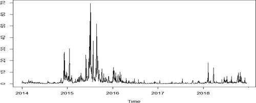
Figure 1 shows the closing price sequence of the CSI 300 index over the sample period. As shown in the figure, the price trend of CSI 300 fluctuates greatly. After a brief rise in early 2015, the price begins to fall sharply in June 2015, and continues to fluctuate thereafter. Figure 2 presents the daily return series of the CSI 300 index. In the figure, the selection of data includes the extreme range, and there is obvious fluctuation aggregation phenomenon, implying that large fluctuations are followed by large fluctuations, and the same applies to small fluctuations. Generally, large fluctuations for a long time, and so do small fluctuations. Figure 3 summarises the daily high-frequency information using the RV. It also depicts the volatility of the full trading days.

Figure 1. Closing price sequence of the CSI 300 index.

Source: authors.

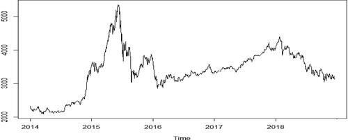
Figure 2. Daily return series of the CSI 300 index.

Source: authors.

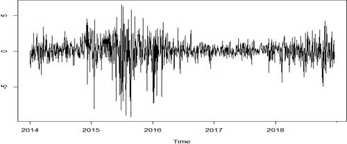
Figure 3. Realized volatility.

Source: authors.

4.2. Parameter estimation results

Hansen and Lunde (2005) and Hansen et al. (2012) show that the GARCH (1) model and the Realized GARCH (1) model have good estimation effect. Therefore, this section builds the GARCH (1) and Realized GARCH (1) models on the basis of the CSI 300 index data.

In this article, we use the maximum likelihood estimation method to estimate the parameters of the GARCH and Realized GARCH models, and the residual terms following the normal and skewed-t distributions, respectively. Table 2 shows the parameter estimation results of the GARCH model, and the p-values of each parameter are less than 0.05, indicating that the parameter values estimated by the model are significant, suggesting that the model has a good fitting effect. The sum of the parameters $\gamma$ and $\beta$ of the GARCH model is less than 1 but very close to 1, indicating that stock return series has strong volatility persistence. In particular, the degree-of-freedom parameter n of the GARCH model based on the skewed-t distribution is equal to 4.5667, indicating that the distribution of the daily return residual shows fat tail phenomenon. The skewness parameter $\lambda$ is equal to 0.9998 and greater than 0, which means that the distribution of the daily return residuals is right-skewed.

Table 2. Estimation results of GARCH model parameters.

Residual distribution	$\omega$	$\gamma$	$\beta$	$n$	$\lambda$
Normal distribution	0.0076 (0.0304)	0.0688 (0.0000)	0.9302 (0.0000)	/	/
Skewed-t distribution	0.0122 (0.0223)	0.0739 (0.0000)	0.9251 (0.0000)	4.5667 (0.0000)	0.9998 (0.0000)

Note: the numbers in brackets in the table refer to the p-value of each parameter.

Source: authors.

Table 3 shows the parameter estimation results of Realized GARCH model based on normal and skewed-t distributions at the 5% significance level, where each parameter estimation of the model is significant. The value of $\beta +\varphi \gamma$ is close to 1, reflecting the persistence of stock return volatility. Regardless of whether the model is based on normal distribution or skewed-t distribution, the coefficients ${\tau }_1$ and ${\tau }_2$ of the lever function are significant and are positive and negative, indicating that the return series has a significant leverage effect. In the two Realized GARCH models, $\beta >\gamma >0$ indicates that the positive contribution of the previous conditional variance to the current conditional variance is higher than that of the realized measure. In particular, the degree-of-freedom parameter n of the Realized GARCH model based on the skewed-t distribution is equal to 4.6654, indicating that the distribution of the daily return residual shows fat tail phenomenon; and skewness parameter $\lambda =0.9650>0$ indicates that the distribution of the daily return residuals is right-biased, consistent with the GARCH model based on skewed-t distribution.

Table 3. Estimation results of Realized GARCH model parameters.

Residual cdistribution	$\omega$	$\gamma$	$\beta$	$\xi$	$\phi$	${\tau }_1$	${\tau }_2$	${\sigma }_u^2$	$n$	$\lambda$
Normal distribution	0.1308 (0.0000)	0.2932 (0.0000)	0.7033 (0.0000)	−0.4223 (0.0000)	0.9539 (0.0000)	−0.0458 (0.0079)	0.1385 (0.0000)	0.5568 (0.0000)	/	/
Skewed-t distribution	0.1506 (0.0000)	0.3070 (0.0000)	0.6859 (0.0000)	−0.4573 (0.0000)	0.9608 (0.0000)	−0.0454 (0.0086)	0.1429 (0.0000)	0.5565 (0.0000)	4.6654 (0.0000)	0.9650 (0.0000)

Note: the numbers in brackets in the table refer to the p-value of each parameter.

Source: authors.

4.3. Out-of-sample volatility forecast

In this article, we divide the sample data into two parts, namely in-sample and out-of-sample. The in-sample data covers 812 data points from January 2, 2014 to May 3, 2017, and the out-of-sample data covers the remaining 400 data points from May 4, 2017 to December 18, 2018. We use rolling time window to predict the out-of-sample volatility. The specific steps are as follows: (1) use the time windows $1,2,\dots ,T_1$ to estimate the parameters and forecast the volatility on day $T_1+1;$ (2) use the time window samples $2,3,\dots ,T_1+1$ to estimate the parameters and forecast the volatility on day $T_1+2;$ (3) re-peat the operation until the time window samples $T-T_1,\dots ,T-1$ are used to estimate the parameters and predict the volatility on day $T.$ Thus, we obtain the $N=T-T_1$ day volatility prediction sequence, where $T=1212,T_1=812,N=400.$

As discussed in Section 3.3, the validity of the MF-MoP model depends on the existence of momentum of predictability, and the dependence between $p{p}_t$ and $c{p}_t$ indicates the existence of momentum of predictability. We use the Pesaran and Timmermann (PT) statistic to test the MF-MoP model, that is, to test the cross-dependence between $p{p}_t$ and $c{p}_t.$ Table 4 shows Pesaran and Timmermann test statistics and p-values. At the 1% significance level, the null hypothesis is rejected, indicating that there is dependence between $p{p}_t$ and $c{p}_t.$ This means that a good past performance can consistently lead to a good current performance, indicating that there indeed exists a momentum of predictability between the GARCH and Realized GARCH models.

Table 4. The results of the PT test.

	Normal distribution	Skewed-t distribution
Statistic	4.6507	4.9684
p-value	0.0000	0.0000

Source: authors.

Based on normal and skewed-t distribution, we can get six volatility models. We use loss function and MCS test to compare the volatility prediction accuracy of these models. Table 5 shows the four groups of loss function values for the out-of-sample volatility prediction of each model. The following results are obtained: (1) Under the four loss function standards, compared to the GARCH model that only considers low-frequency data, the loss function values of the Realized GARCH model that considers high-frequency data are relatively small. The four loss function values of the MF-MoP model based on mixed-frequency data are the smallest, indicating that this model based on low-frequency information and high-frequency information has the minimum prediction loss. (2) From the perspective of the asymmetric and fat-tailed distribution, the skewed-t distribution is considered to be more accurate in describing the typical characteristics of financial data, such as asymmetry and fat tail. Therefore, all models based on skewed-t distribution are taken as comparative models. The loss function values of the GARCH, Realized GARCH and MF-MoP models based on skewed-t distribution are smaller than those of the same three models based on normal distribution. This suggests that the four loss function values (MAE, MSPE, MAPE and R2LOG) for the models based on skewed-t distribution are all smaller than those based on normal distribution. Among them, the MF-MoP model based on the skewed-t distribution has the smallest loss function under the loss function MAE, MSPE, MAPE and R2LOG, indicating that the prediction error of this model is relatively small. To obtain more robust and scientific results, it is necessary to further test the prediction results.

Table 5. Loss function value of volatility prediction.

Model	Distribution	MAE	MSPE	MAPE	R2LOG
GARCH	Normal	0.8808	2.2323	1.0793	0.7042
	Skewed-t	0.8447	1.9115	0.9784	0.6699
Realized GARCH	Normal	0.8234	2.1825	1.0409	0.6375
	Skewed-t	0.7740	1.8274	0.9400	0.5797
MF-MoP	Normal	0.8078	1.9406	0.9577	0.6026
	Skewed-t	0.7636	1.6018	0.8660	0.5560

Source: authors.

Therefore, to better test the volatility prediction ability of the MF-MoP model, we conduct MCS tests on the GARCH, Realized GARCH and MF-MoP models. In the MCS test, we set the significance level of 0.1, indicating that the prediction performance of the model with a p-value less than 0.1 is significantly worse than that of other models in the MCS test. Such a model will be eliminated in the process of the MCS test. The volatility prediction model with a p-value greater than 0.1 is a model with good out-of-sample prediction ability and can survive the MCS test; the larger is the p-value, the higher is the volatility prediction accuracy of the model. If the p-value of the model is equal to 1, the model is considered to be the optimal volatility model in the MCS test set.

To obtain the p-value of the MCS test, we set the block length to 2 and simulation times to 10000 as the control parameters of the Bootstrap process. Table 6 shows the MCS test results of different volatility models, presenting the following: (1) under any loss function, the p-value of the MF-MoP model based on skewed-t distribution is 1, indicating that this model is the most optimal model among the six volatility models. (2) On the whole, under the assumption of the same residual distribution, the p-value of the MF-MoP model is higher than that of the GARCH or the Realized GARCH models, indicating that the MF-MoP model combining low-frequency and high-frequency information can improve the prediction accuracy of volatility. It also indicates that the MF-MoP model is robust under different distribution assumptions. In addition, under the premise of the same volatility model, the model considering the fat-tailed distribution has better prediction performance. Among them, the MF-MoP model based on the skewed-t distribution passes the MCS test, and has better prediction effect than the MF-Mop model based on normal distribution. This shows that the model based on skewed-t distribution can accurately describe the asymmetric thick-tailed characteristics of financial data.

Table 6. The results of MCS test.

Model	Distribution	MAE		MSPE		MAPE		R2LOG
		$T_{SQ}$	$T_R$	$T_{SQ}$	$T_R$	$T_{SQ}$	$T_R$	$T_{SQ}$	$T_R$
GARCH	Normal	0.0000	0.0000	0.0000	0.0000	0.0000	0.0000	0.0000	0.0000
	Skewed-t	0.4912	0.0000	0.8152	0.0000	0.6532	0.0000	0.2786	0.0000
Realized GARCH	Normal	0.4060	0.0000	0.0000	0.0000	0.0000	0.0000	0.3874	0.0000
	Skewed-t	1.0000	0.5328	0.9992	0.0000	0.9952	0.0000	1.0000	0.1674
MF-MoP	Normal	0.9564	0.0000	0.2076	0.0000	0.4996	0.0000	1.0000	0.0000
	Skewed-t	1.0000	1.0000	1.0000	1.0000	1.0000	1.0000	1.0000	1.0000

Note: bold font indicates the best volatility model, and p-value less than 0.1 indicates that the model is rejected by MCS test at 10% significance level.

Source: authors.

5. Robustness test

To illustrate the advantages of the MF-MoP model, this article verifies the robustness of the MF-MoP model based on different realized measures, look-back periods and stock data.

5.1. Different realized measures

First, considering the impact of microstructural noise and volatility jumps on the volatility forecast in the stock market, we introduce realized range volatility (RRV) and realized median volatility (MedRV) into the model to verify whether the empirical results of the MF-MoP model based on different realized measures are robust. The RRV proposed by Christensen and Podolskij (2007) can effectively solve the market microstructure noise, and is defined as follows: (24) $$RR{V}_t=\frac{1}{4\hspace{0.17em}\text{ln}\hspace{0.17em}2}\sum _{i=1}^m{(\hspace{0.17em}\text{ln}\hspace{0.17em}{H}_{t,i}-\hspace{0.17em}\text{ln}\hspace{0.17em}{L}_{t,i})}^2$$(24) where $H_{t,i}$ and $L_{t,i}$ are the highest and lowest prices of the stocks of the ith collection point on day t, and m is the daily sampling frequency of high-frequency data.

The MedRV, proposed by Andersen et al. (2012), is robust for stock micro-structure noise and jumping behaviour, which is defined as follows: (25) $$\mathit{MedR}{V}_t=\frac{\pi }{6-4\sqrt{3}+\pi }\left(\frac{m}{m-2}\right)\sum _{i=2}^{m-1}\mathit{med}{\left(\left|r_{t,i-1}\right|,\left|r_{t,i}\right|,\left|r_{t,i+1}\right|\right)}^2$$(25) where $r_{t,\mathrm{ }i}$ is the stock return rate at the ith collection point on day t, and m is the daily sampling frequency of high-frequency data.

This chapter uses the empirical data from Section 3 to establish volatility prediction models based on RRV and MedRV. First, we use PT statistics to test whether the MF-MoP model based on different realized measures has the momentum of predictability. Table 7 shows the results of the PT test for different realized measures. It is evident that regardless of the realized measure being RRV or MedRV, the p-values of the model are less than 0.01, rejecting the null hypothesis that the two time series of $p{p}_t$ and $c{p}_t$ are independent in the presence of serial dependencies. Thus, there is a momentum of predictability between the GARCH and Realized GARCH models based on the realized measures of RRV and MedRV.

Table 7. The results of PT test for different realized measures.

	RRV		MedRV
	Normal distribution	Skewed-t distribution	Normal distribution	Skewed-t distribution
Statistic	9.6135	9.2637	8.6095	8.4814
p-value	0.0000	0.0000	0.0000	0.0000

Source: authors.

Table 8 shows the MCS test results of the six prediction models based on RRV and MedRV. The results show that the p-value of the MF-MoP model based on the skewed-t distribution is 1 whether RRV or MedRV is used, indicating that the MF-MoP model based on the skewed-t distribution is the optimal model from the six volatility models. Second, based on the perspective of the asymmetric thick-tailed distribution, the skewed-t distribution can more accurately describe the typical factual characteristics of financial data such as the asymmetric thick tail. Thus, we take various models based on the skewed-t distribution as comparison models. The p-value of the MF-MoP model is greater than that of the GARCH and the Realized GARCH models, indicating that the MF-MoP model has higher volatility prediction accuracy and that the volatility prediction effect of the MF-MoP model is robust under different realized measures.

Table 8. MCS test results of different realized measures.

Model	Distribution	MAE		MSPE		MAPE		R2LOG
		$T_{SQ}$	$T_R$	$T_{SQ}$	$T_R$	$T_{SQ}$	$T_R$	$T_{SQ}$	$T_R$
RRV
GARCH	Normal	0.0000	0.0000	0.0000	0.0000	0.0000	0.0000	0.0000	0.0000
	Skewed-t	0.3676	0.0000	0.0000	0.0000	0.0000	0.0000	0.0000	0.0000
Realized GARCH	Normal	0.1878	0.0000	0.0000	0.0000	0.0000	0.0000	0.0000	0.0000
	Skewed-t	0.9998	0.0000	0.0000	0.0000	0.0000	0.0000	0.0000	0.0000
MF-MoP	Normal	1.0000	0.0000	0.0000	0.0000	0.0000	0.0000	0.0000	0.0000
	Skewed-t	1.0000	1.0000	1.0000	1.0000	1.0000	1.0000	1.0000	1.0000
MedRV
GARCH	Normal	0.0000	0.0000	0.0000	0.0000	0.0000	0.0000	0.0000	0.0000
	Skewed-t	0.0000	0.0000	0.2892	0.0000	0.0000	0.0000	0.1634	0.0000
Realized GARCH	Normal	0.0000	0.0000	0.4110	0.0000	0.0000	0.0000	0.1108	0.0000
	Skewed-t	0.0000	0.0000	1.0000	0.0000	0.0000	0.0000	1.0000	0.0000
MF-MoP	Normal	0.0000	0.0000	1.0000	0.0000	0.0000	0.0000	1.0000	0.0000
	Skewed-t	1.0000	1.0000	1.0000	1.0000	1.0000	1.0000	1.0000	1.0000

Note: bold font indicates the best volatility model, and p-value less than 0.1 indicates that the model is rejected by MCS test at 10% significance level.

Source: authors.

5.2. Different look-back periods

The prediction of the MF-MoP model is to switch between the prediction of the GARCH model and the Realized GARCH model to generate a new prediction, which depends on their recent past performance, and the past forecasting performance is affected by the choice of look-back periods. Therefore, we test the volatility prediction performance of the MF-MoP model for look-back periods with k = 1,3,6.

Table 9 shows the results of the Pesaran and Timmermann tests in look-back periods. When the look-back periods k = 1,3,6, the MF-MoP model rejects the original hypothesis at the 1% significance level, indicating that $p{p}_t$ and $c{p}_t$ are interdependent. Therefore, a better past performance can consistently lead to a better current performance, suggesting that momentum of predictability exists in MF-MoP model under different look-back periods.

Table 9. The results of PT test in different look-back periods.

	k = 1		k = 3		k = 6
	Normal distribution	Skewed-t distribution	Normal distribution	Skewed-t distribution	Normal distribution	Skewed-t distribution
Statistic	6.3503	7.6864	6.9398	7.7582	5.9361	6.8244
p-value	0.0000	0.0000	0.0000	0.0000	0.0000	0.0000

Source: authors.

Table 10 shows the MCS test results of the six prediction models used in different look-back periods. The results show that, in the look-back periods k = 1,3,6, the MCS test of the MF-MoP model based on the skewed-t distribution, always produces the largest p-value of 1, while the remaining models cannot always pass the MCS test. In other words, the MF-MoP model based on the skewed-t distribution is more likely to be the best model for volatility prediction, that is, the volatility prediction ability of the MF-MoP model is robust under different look-back periods.

Table 10. The results of MCS test in different look-back periods.

Model	Distribution	MAE		MSPE		MAPE		R2LOG
		$T_{SQ}$	$T_R$	$T_{SQ}$	$T_R$	$T_{SQ}$	$T_R$	$T_{SQ}$	$T_R$
k = 1
GARCH	Normal	0.0000	0.0000	0.0000	0.0000	0.0000	0.0000	0.0000	0.0000
	Skewed-t	0.0000	0.0000	0.0000	0.0000	0.2662	0.0000	0.1538	0.0000
Realized GARCH	Normal	0.0000	0.0000	0.0000	0.0000	0.0000	0.0000	0.1708	0.0000
	Skewed-t	0.0000	0.0000	0.0000	0.0000	0.4810	0.0000	1.0000	0.0000
MF-MoP	Normal	0.0000	0.0000	0.0000	0.0000	1.0000	0.0000	1.0000	0.0000
	Skewed-t	1.0000	1.0000	1.0000	1.0000	1.0000	1.0000	1.0000	1.0000
k = 3
GARCH	Normal	0.0000	0.0000	0.0000	0.0000	0.0000	0.0000	0.0000	0.0000
	Skewed-t	0.0000	0.0000	0.6270	0.0000	0.2062	0.0000	0.1634	0.0000
Realized GARCH	Normal	0.0000	0.0000	0.0000	0.0000	0.0000	0.0000	0.1108	0.0000
	Skewed-t	0.3250	0.0000	0.7164	0.0000	0.5560	0.0000	1.0000	0.0000
MF-MoP	Normal	0.1238	0.0000	0.6290	0.0000	0.9886	0.0000	1.0000	0.0000
	Skewed-t	1.0000	1.0000	1.0000	1.0000	1.0000	1.0000	1.0000	1.0000
k = 6
GARCH	Normal	0.0000	0.0000	0.1028	0.0000	0.0000	0.0000	0.0000	0.0000
	Skewed-t	0.2436	0.0000	1.0000	0.0000	0.1728	0.0000	0.2200	0.0000
Realized GARCH	Normal	0.1668	0.0000	0.1112	0.0000	0.0000	0.0000	0.2632	0.0000
	Skewed-t	1.0000	0.1134	1.0000	0.0000	0.8918	0.0000	1.0000	0.0000
MF-MoP	Normal	1.0000	0.0000	1.0000	0.0000	0.4638	0.0000	1.0000	0.0000
	Skewed-t	1.0000	1.0000	1.0000	1.0000	1.0000	1.0000	1.0000	1.0000

Note: bold font indicates the best volatility model, and p-value less than 0.1 indicates that the model is rejected by MCS test at the 10% significance level.

Source: authors.

5.3. Different stock data

In this section, we consider the CSI 300 index (the representative stock index of China), the N225 index (the representative stock index of Japan) and the KS11 index (the representative stock index of South Korea), which are widely used in stock volatility forecasting. To illustrate that our results do not depend on the selection of time periods, we select the data from 1 January 2014 to 31 December 2021. Note that the COVID-19 pandemic took place during this period, and therefore, it is even more meaningful to study it. The data of N225 and KS11 indexes are obtained from the Oxford-Man Institute of Quantitative Finance. Additionally, the sample length is 2000 and the rolling prediction length is 400.

Table 11 presents the results of Pesaran and Timmermann tests of different data. It is evident that the MF-MoP model also has the momentum of predictability under the data of the KS11, N225 and CSI 300 indexes. To illustrate the influence of different data on model results, the results of the MCS test are presented in Table 12. It can be seen that under most stock indexes and various loss function indexes, the p-values of the MF-MoP model based on the skewed-t distribution are far greater than that of other models. In other words, the MF-MoP model based on the skewed-t distribution is never eliminated by the MCS procedure. In contrast, the GARCH model is usually discarded by the MCS test. Compared to the GARCH model, the Realized GARCH model shows larger p-values, but the model cannot always enter MCS. In summary, the out-of-sample prediction performance of the MF-MoP model considering fat-tailed distribution is significantly better than that of other models, which is consistent with the previous research results.

Table 11. The results of PT test of different data.

	KS11		N225		CSI 300
	Normal distribution	Skewed-t distribution	Normal distribution	Skewed-t distribution	Normal distribution	Skewed-t distribution
Statistic	2.3331	5.9391	6.8122	5.6643	3.2784	4.1794
p-value	0.0098	0.0000	0.0000	0.0000	0.0000	0.0000

Source: authors.

Table 12. MCS test results of different data.

Model	Distribution	MAE		MSPE		MAPE		R2LOG
		$T_{SQ}$	$T_R$	$T_{SQ}$	$T_R$	$T_{SQ}$	$T_R$	$T_{SQ}$	$T_R$
KS11
GARCH	Normal	0.0000	0.0000	0.9978	0.0000	0.0000	0.0000	0.0000	0.0000
	Skewed-t	0.0000	0.0000	0.3490	0.2198	0.0000	0.0000	0.0000	0.0000
Realized GARCH	Normal	0.0000	0.0000	1.0000	0.0000	0.0000	0.0000	0.0000	0.0000
	Skewed-t	0.9226	0.3856	1.0000	1.0000	0.3570	0.3536	1.0000	0.4226
MF-MoP	Normal	0.4010	0.0000	1.0000	1.0000	0.0000	0.0000	0.1794	0.0000
	Skewed-t	1.0000	1.0000	1.0000	1.0000	1.0000	1.0000	1.0000	1.0000
N225
GARCH	Normal	0.0000	0.0000	0.2008	0.0000	0.2120	0.0000	0.2938	0.0000
	Skewed-t	0.0000	0.0000	0.0000	0.0000	0.0000	0.0000	0.0000	0.0000
Realized GARCH	Normal	0.0000	0.0000	0.0000	0.0000	0.0000	0.0000	0.0000	0.0000
	Skewed-t	0.0000	0.0000	0.2008	0.0000	0.7384	0.0000	0.5518	0.0000
MF-MoP	Normal	1.0000	1.0000	0.5742	0.0000	1.0000	0.2406	0.9260	0.4658
	Skewed-t	0.9928	0.745	1.0000	1.0000	1.0000	1.0000	1.0000	1.0000
CSI 300
GARCH	Normal	0.0000	0.0000	0.0000	0.0000	0.0000	0.0000	0.2650	0.0000
	Skewed-t	0.0000	0.0000	0.0000	0.0000	0.0000	0.0000	0.3010	0.0000
Realized GARCH	Normal	0.8010	0.7974	0.0000	0.0000	0.4544	0.4714	1.0000	1.0000
	Skewed-t	0.9890	0.9872	0.8986	0.9066	1.0000	1.0000	0.8674	0.5014
MF-MoP	Normal	0.9958	0.9934	0.0000	0.0000	0.1964	0.1986	1.0000	1.0000
	Skewed-t	1.0000	1.0000	1.0000	1.0000	1.0000	1.0000	0.8792	0.5252

Note: bold font indicates the best volatility model, and p-value less than 0.1 indicates that the model is rejected by MCS test at 10% significance level.

Source: authors.

6. Conclusion

In this article, we introduce the momentum of predictability proposed by Wang et al. (2018) to combine the GARCH model based on low-frequency data, with the Realized GARCH model based on high-frequency data. Subsequently, we construct a mixed-frequency model based on the momentum of predictability to describe the interaction process between low-frequency and high-frequency volatility. The CSI 300 index data are selected as the research object to conduct empirical tests on the model. We use the rolling time window method to make out-of-sample forecasts of volatility, and implement four loss function evaluation indicators and the MCS test to compare the volatility prediction effect of the GARCH, Realized GARCH and MF-MoP models. Finally, we discuss the robustness of the MF-MoP model under different look-back periods, stock data and realized measures, and the following conclusions are obtained.

First, compared to the traditional GARCH model based on low-frequency data and the Realized GARCH model based on high-frequency data, the MF-MoP model combining low-frequency and high-frequency data has higher volatility prediction accuracy. This demonstrates that our proposed models can achieve better performances in forecasting volatility. Second, the out-of-sample findings based on four loss function criteria and the MCS test suggest that the MF-MoP model based on the skewed-t distribution has better prediction effect than the model based on normal distribution. Thus, considering the asymmetric fat-tailed distribution in volatility, the MF-MoP model can improve the prediction effect of volatility, which is consistent with the previous related research results. Third, according to the robustness test, these conclusions are robust to different look-back periods, realized measures and stock data. Finally, through the Pesaran and Timmermann test, it is proved that momentum of predictability does exist in the MF-MoP model, which further confirms its effectiveness.

This research provides a new tool for investors and managers to understand stock market volatility. Naturally, we can extend this research by using other basic models, such as the TGARCH model and Realized HAR GARCH model. We leave this to future research.

Disclosure statement

No conflict of interest has been declared by the authors.

Additional information

Funding

This work was supported by Zhejiang Provincial Natural Science Foun-dation of China (LY21G010003), the National Natural Science Foundation of China (11971432), Zhejiang Provincial Natural Science Foundation of China (LQ22G010001), and the Leading Talent Cultivation Project of Zhejiang Province Philosophy and Social Science Planning (22YJRC07ZD-2YB). This work was also supported by the Characteristic & Preponderant Discipline of Key Construction Universities in Zhejiang Province (Zhejiang Gongshang University-Statistics) and Collaborative Innovation Center of Statistical Data Engineering Technology & Application.

References

- Andersen, T. G., & Bollerslev, T. (1998). Answering the skeptics: Yes, standard volatility models do provide accurate forecasts. International Economic Review, 39(4), 885–905. https://doi.org/10.2307/2527343
- Andersen, T. G., Dobrev, D., & Schaumburg, E. (2012). Jump-robust volatility estimation using nearest neighbor truncation. Journal of Econometrics, 169(1), 75–93. https://doi.org/10.1016/j.jeconom.2012.01.011
- Andreou, E. (2016). On the use of high frequency measures of volatility in MIDAS regressions. Journal of Econometrics, 193(2), 367–389. https://doi.org/10.1016/j.jeconom.2016.04.012
- Baillie, R. T., Bollerslev, T., & Mikkelsen, H. O. (1996). Fractionally integrated generalized autoregressive conditional heteroskedasticity. Journal of Econometrics, 74(1), 3–30. https://doi.org/10.1016/S0304-4076(95)01749-6
- Bollerslev, T. (1986). Generalized autoregressive conditional heteroskedasticity. Journal of Econometrics, 31(3), 307–327. https://doi.org/10.1016/0304-4076(86)90063-1
- Cai, G., Wu, Z., & Peng, L. (2021). Forecasting volatility with outliers in Realized GARCH models. Journal of Forecasting, 40(4), 667–685. https://doi.org/10.1002/for.2736
- Catania, L., & Proietti, T. (2020). Forecasting volatility with time-varying leverage and volatility of volatility effects. International Journal of Forecasting, 36(4), 1301–1317. https://doi.org/10.1016/j.ijforecast.2020.01.003
- Christensen, K., & Podolskij, M. (2007). Realized range-based estimation of integrated variance. Journal of Econometrics, 141(2), 323–349. https://doi.org/10.1016/j.jeconom.2006.06.012
- Corsi, F. (2009). A simple approximate long-memory model of realized volatility. Journal of Financial Econometrics, 7(2), 174–196. https://doi.org/10.1093/jjfinec/nbp001
- Degiannakis, S., & Filis, G. (2022). Oil price volatility forecasts: What do investors need to know? Journal of International Money and Finance, 123, 102594. https://doi.org/10.1016/j.jimonfin.2021.102594
- Hansen, B. E. (1994). Autoregressive conditional density estimation. International Economic Review, 35(3), 705–730. https://doi.org/10.2307/2527081
- Hansen, P. R., Huang, Z., & Shek, H. H. (2012). Realized GARCH: A joint model for returns and realized measures of volatility. Journal of Applied Econometrics, 27(6), 877–906. https://doi.org/10.1002/jae.1234
- Hansen, P. R., & Lunde, A. (2005). A forecast comparison of volatility models: Does anything beat a GARCH(1,1). Journal of Applied Econometrics, 20(7), 873–889. https://doi.org/10.1002/jae.800
- Hansen, P. R., Lunde, A., & Nason, J. M. (2011). The model confidence set. Econometrica, 79(2), 453–497.
- Hongwiengjan, W., & Thongtha, D. (2021). An analytical approximation of option prices via TGARCH model. Economic Research-Ekonomska Istraživanja, 34(1), 948–969. https://doi.org/10.1080/1331677X.2020.1805636
- Hung, J. C., Liu, H. C., & Yang, J. J. (2020). Improving the realized GARCH’s volatility forecast for bitcoin with jump-robust estimators. The North American Journal of Economics and Finance, 52, 101165. https://doi.org/10.1016/j.najef.2020.101165
- Huang, Z., Liu, H., & Wang, T. (2016). Modeling long memory volatility using realized measures of volatility: A realized HAR GARCH model. Economic Modelling, 52, 812–821. https://doi.org/10.1016/j.econmod.2015.10.018
- Jiang, W., Ruan, Q., Li, J., & Li, Y. (2018). Modeling returns volatility: Realized GARCH incorporating realized risk measure. Physica A: Statistical Mechanics and Its Applications, 500, 249–258. https://doi.org/10.1016/j.physa.2018.02.018
- Kim, J. M., Kim, D. H., & Jung, H. (2021). Estimating yield spreads volatility using GARCH-type model. The North American Journal of Economics and Finance, 57, 101396. https://doi.org/10.1016/j.najef.2021.101396
- Liu, L. Y., Patton, A. J., & Sheppard, K. (2015). Does anything beat 5-minute RV? A comparison of realized measures across multiple asset classes. Journal of Econometrics, 187(1), 293–311. https://doi.org/10.1016/j.jeconom.2015.02.008
- Liu, Y., Li, J., & Ng, A. C. (2015). Option pricing under GARCH models with Hansen's skewed-t distributed innovations. The North American Journal of Economics and Finance, 31, 108–125. https://doi.org/10.1016/j.najef.2014.10.007
- Ma, F., Lu, X., Wang, L., & Chevallier, J. (2021). Global economic policy uncertainty and gold futures market volatility: Evidence from Markov regime‐switching GARCH‐MIDAS models. Journal of Forecasting, 40(6), 1070–1085. https://doi.org/10.1002/for.2753
- Mei, D., Ma, F., Liao, Y., & Wang, L. (2020). Geopolitical risk uncertainty and oil future volatility: Evidence from MIDAS models. Energy Economics, 86, 104624. https://doi.org/10.1016/j.eneco.2019.104624
- Miao, H., Ramchander, S., Wang, T., & Yang, D. (2017). Role of index futures on China’s stock markets: Evidence from price discovery and volatility spillover. Pacific-Basin Finance Journal, 44, 13–26. https://doi.org/10.1016/j.pacfin.2017.05.003
- Nelson, D. B. (1991). Conditional heteroskedasticity in asset returns: A new approach. Econometrica, 59(2), 347. https://doi.org/10.2307/2938260
- Pesaran, M. H., & Timmermann, A. (2009). Testing dependence among serially correlated multicategory variables. Journal of the American Statistical Association, 104(485), 325–337. https://doi.org/10.1198/jasa.2009.0113
- Qiao, G., Teng, Y., Li, W., & Liu, W. (2019). Improving volatility forecasting based on Chinese volatility index information: Evidence from CSI 300 index and futures markets. The North American Journal of Economics and Finance, 49, 133–151. https://doi.org/10.1016/j.najef.2019.04.003
- Shang, Y., & Zheng, T. (2021). Mixed-frequency SV model for stock volatility and macroeconomics. Economic Modelling, 95, 462–472. https://doi.org/10.1016/j.econmod.2020.03.013
- Smetanina, E. (2017). Real-time GARCH. Journal of Financial Econometrics, 15(4), 561–601. https://doi.org/10.1093/jjfinec/nbx008
- Tian, S., & Hamori, S. (2015). Modeling interest rate volatility: A Realized GARCH approach. Journal of Banking & Finance, 61, 158–171. https://doi.org/10.1016/j.jbankfin.2015.09.008
- Wang, L., Ma, F., Liu, J., & Yang, L. (2020). Forecasting stock price volatility: New evidence from the GARCH-MIDAS model. International Journal of Forecasting, 36(2), 684–694. https://doi.org/10.1016/j.ijforecast.2019.08.005
- Wang, Y., Liu, L., Ma, F., & Diao, X. (2018). Momentum of return predictability. Journal of Empirical Finance, 45, 141–156. https://doi.org/10.1016/j.jempfin.2017.11.003
- Wang, Y., & Wu, C. (2012). Forecasting energy market volatility using GARCH models: Can multivariate models beat univariate models? Energy Economics, 34(6), 2167–2181. https://doi.org/10.1016/j.eneco.2012.03.010
- Wang, Y., Xiang, Y., Lei, X., & Zhou, Y. (2022). Volatility analysis based on GARCH-type models: Evidence from the Chinese stock market. Economic Research-Ekonomska Istraživanja, 35(1), 2530–2554. https://doi.org/10.1080/1331677X.2021.1967771
- Wu, X., Xia, M., & Zhang, H. (2020). Forecasting VaR using realized EGARCH model with skewness and kurtosis. Finance Research Letters, 32, 101090. https://doi.org/10.1016/j.frl.2019.01.002
- Yu, J. (2005). On leverage in a stochastic volatility model. Journal of Econometrics, 127(2), 165–178. https://doi.org/10.1016/j.jeconom.2004.08.002
- Yu, X., & Huang, Y. (2021). The impact of economic policy uncertainty on stock volatility: Evidence from GARCH–MIDAS approach. Physica A: Statistical Mechanics and Its Applications, 570, 125794. https://doi.org/10.1016/j.physa.2021.125794
- Zhang, N., Wang, A., Haq, Naveed-Ul., & Nosheen, S. (2022). The impact of COVID-19 shocks on the volatility of stock markets in technologically advanced countries. Economic Research-Ekonomska Istraživanja, 35(1), 2191–2216. https://doi.org/10.1080/1331677X.2021.1936112
- Zhang, Y., Ma, F., Wang, T., & Liu, L. (2019). Out-of-sample volatility prediction: A new mixed‐frequency approach. Journal of Forecasting, 38(7), 669–680. https://doi.org/10.1002/for.2590