The effects of education upward mobility on income upward mobility: evidence from China

Abstract

The effect of education on income has been debated in recent years. We use the China Health and Nutrition Survey database to research the relationship between education upward mobility and income upward mobility. We find education upward mobility has a positive effect on income upward mobility. The intergenerational psychological distance which is a measure of the difference between parents’ and children’s conceptualizations, parents’ social capital, and children’s gender all have effects on this relationship. To be specific, the positive effect is reinforced by a certain amount of intergenerational psychological distance, but is negated by an excessive amount of intergenerational psychological distance. Besides, education upward mobility actively increases the income upward mobility of rural-dwelling children whose parents lack social capital, i.e., education is a key factor that improves the income of children from rural families. In contrast, education upward mobility only actively increases the income upward mobility of urban-dwelling children whose parents have social capital. In addition, the positive effect of education on children’s income is more evident in boys than in girls. These findings greatly advance our understanding of the beneficial effects of education on the income, and will assist improvements to be made in these areas.

Keywords:

• Education upward mobility
• income upward mobility
• intergenerational psychological distance
• social capital

JEL CODES:

• J31
• J62
• O10

1. Introduction

Numerous studies explore how income can be increased (Darku & Yeboah, 2018; Égert et al., 2020; Holcombe & Lacombe, 2004; Islam, 1996; Mincer, 1974; Thurow, 1970). In many developing countries, such as China, increasing people’s number of years of schooling is typically regarded as the most effective way to increase their income (Blomstrom et al., 1992; Coady & Dizioli, 2018; Jolliffe, 2002). However, scholars disagree on whether education does indeed increase people’s income. Some scholars find that education has a critical effect on intergenerational income transmission, by providing more possibilities for increases in children’s income (Fan, 2016; Gong et al., 2012; Palomino et al., 2018; Yuan, 2017). Other scholars argue that education has little effect on children’s income (Blanden, 2013; Narayan et al., 2018; Yuan & Chen, 2013). Thus, it appears that whether education increases children’s income may depend on their societal situation. Therefore, whether increasing Chinese children’s years of education increases their income remains an open question. For this reason, this paper discusses whether increasing the education of children leads to their having higher incomes than their parents, which is crucial for understanding whether increasing children’s education could increase national income levels in China.

Mobility researches study the correlation and change of income between generations and it has two stands: relative income mobility (Fan, 2016; Solon, 1992, 1999), which is also called intergenerational transmission or intergeneration mobility. It measures the correlation between different generations and scholars usually study to what extent children’s income or education level depend their parents’ income or education level (Chetty et al., 2017; Becker & Tomes, 1979). The other stand is absolute income mobility (Checchi et al., 1999; Chetty et al., 2014, 2020), also called upward mobility (Chetty et al., 2014), which measures whether children’s absolute number or rank surpass their parents (income or education levels). Most studies tend to focus on the effect of education on relative income mobility (Bowles & Gintis, 2002; Fan, 2016; Guo & Min, 2008; Lefgren et al., 2012; Yang & Qiu, 2016). Children of parents with higher educational levels themselves have higher educational levels (Yang, 2016), as well as higher cognitive levels and social skills (Narayan et al., 2018), than children of parents with lower educational levels, and thus have higher incomes. Wang et al. (2022) show more evidences that the effects of education on intergenerational income mobility and find that the return on education has stronger explanatory power on intergenerational income mobility than the correlation between a father’s income and his child’s education in China. In addition, it has been claimed that education policy affects relative income mobility (Pekkarinen et al., 2009). However, Blanden (2013) shows that education has little effect on relative income mobility in the USA and the UK. Narayan et al. (2018) obtain a similar result by an empirical analysis of data from 41 developing countries and eight developed countries. Nevertheless, research on these relationships may not be robust, as the measurement of relative mobility is unstable, and thus absolute mobility is probably a more valid measurement (Chetty et al., 2014). The aforementioned studies of relative income mobility therefore stimulate our interest in studying absolute income mobility, in particular because the effect of upward mobility in education on income upward mobility has been neglected, despite the fact that this effect can more clearly reveal whether children’s incomes surpass those of their parents (Chetty et al., 2014, 2020).

This issue is of particular practical importance in China, as it is the largest developing country in the world, and strives to avoid the middle-income trap. As such, the Chinese government has endeavored for many years to help the population of China to achieve income upward mobility, and thereby to lift people out of poverty and promote national economic development so as to avoid the middle-income trap. In China, education is traditionally regarded as critical for poverty alleviation and increasing incomes (Eryong & Xiuping, 2018; Song et al., 2012), and the Chinese government has thus increased investment in education, provides free compulsory education, and prioritizes the admission of poor students to schools to raise the educational levels of the younger generation (Liu et al., 2020). However, it remains to be verified whether such efforts promote income upward mobility, and thereby enhance the overall development of the Chinese economy. Furthermore, there are great differences between developing countries and developed countries in terms of educational systems and educational development processes, and the related researches carried out in developed countries are much more than those in developing countries. In addition, the achievements of researches conducted by developed countries are not easy to be adopted by developing countries. Therefore, conducting this research in China which is the largest developing country in the world can not only provide more conclusions for the research field, but also can provide more adoptable achievements for many other developing countries. Accordingly, we study whether Chinese children’s upward education mobility leads to income upward mobility.

The main contributions of this paper are as follows. First, we study the direct effect of upward education mobility on income upward mobility to determine whether increasing children’s educational level can lead to children earning more than their parents. Specifically, we analyze how children outperform their parents, beyond having a greater income. Other studies usually examine the relationship between education upward mobility and income upward mobility separately (Blanden & Machin, 2013; Cole & Omari, 2003; Gang et al., 2002; Kearney & Levine, 2014; Sturgis & Buscha, 2015). For example, Guo and Min (2008) analyzes the role of education in elevating children into the highest income group, and provide the evidences that education will improve children’s chances of getting into the highest-income group, i.e., the income upward mobility that aims for highest-income group. Chetty et al. (2014) and Chetty et al. (2020) use combined data from the USA to study changes in income upward mobility, and find that this change is affected by location, race, family relationships, and gender. Guo et al. (2019) study China, revealing that college expansion policies and the Compulsory Education Law increase the probability of education upward mobility. However, they do not study the link between education upward mobility and income upward mobility, and more exploration of the relationship between these two aspects is required. In addition, the similar study (Guo & Min, 2008) prove that increase length of education of children of Chinese urban households, in particular those from low-income families, helps elevate them into the highest-income group. However, the improvements for both urban and rural children to get into any higher-income group (compared to income group they would have been) are worth studying, and there are limitations to studying the chance for only urban children to get into the highest-income groups. I expand the research sample to include both rural and urban samples, and I adopt new measures for upward mobility (It is explained in the third of main contributions). Our research is therefore an important complement to the above literature, and deepens current understanding of the ability of education to increase incomes.

Notably, we strengthen our analysis by considering the actual situation in China: this involves studying China’s unique hukou system, which restricts the flow of people between urban and rural areas (Liu, 2005). Liu et al. (2013) find a significant difference between the incomes of people in urban and rural areas. Moreover, other researchers find that the status of education (Rao & Ye, 2016) and the development model (Song et al., 2012; Zheng & Yu, 2011) in urban areas differs from those in rural areas. As these differences may affect the relationship between upward educational mobility and income upward mobility in these areas, we divide our sample into an urban panel and a rural panel according to people’s hukou, as Guo et al. (2019) do, and perform a comparative analysis. We also analyze the effects of other important factors on the relationship between education upward mobility and income upward mobility, such as parents’ social capital and children’s gender, as other researchers show that these factors have a significant effect on education or income. For example, Gang et al. (2002) study the influence of gender on income upward mobility, while Chetty et al. (2014, 2020) find that regional and social capital indices can affect income upward mobility. Through this research, we find that education upward mobility has a robust, positive effect on income upward mobility, such that children have a higher income than their elders, due to receiving more education than their elders.

Second, as few researchers perform a micro-perspective examination of income upward mobility, we do so by using personal household data from the China Health and Nutrition Survey. Micro-perspective research can better capture individual differences and thus afford more realistic results than macro-perspective research. Accordingly, we comprehensively consider the influence of heterogeneity, in terms of the intergenerational psychological distance between parents and children, the social capital of parents, and the gender of children. In contrast, several groups of researchers perform macro-perspective research, by calculating the proportion of income upward mobility in terms of the percentages of children earning more than their parents in particular areas of the world, thereby revealing the difficulty of realizing income upward mobility (Acs et al., 2016; Chetty et al., 2017; Isaacs et al., 2008; Urahn et al., 2012). For example, Acs et al. (2016) find that 63% of children in the USA earn more than their parents, but Chetty et al. (2017) find that absolute income mobility decreases over time in the USA, and that this is related to macroeconomic development.

Third, we capture additional information by adopting new measures for income upward mobility and education upward mobility. Specifically, we use the difference between the income and number of school years of children and their parents to measure both types of upward mobility, which reveals the existence and magnitude of upward mobility. In previous research, Checchi et al. (1999) and Majumder (2010) measure upward mobility using a dummy variable that is equal to 1 if children surpass their parents in a specific factor, and 0 otherwise. However, this measurement can only reveal the existence of upward mobility; in contrast, our measurement generates two pieces of information. That is, (i) the sign of the difference between children and parents’ income and number of school years, which reveals whether upward mobility exists (positive sign = yes; negative sign or 0 = no), and (ii) we get the information about the extent of upward mobility or the gap between children and parents by calculating the accurate difference in the value of schooling years or income between the children and the parents. The positive difference in the value denotes the exact extent of upward mobility. As this point, realizing the upward mobility can be thought as enhancing the extent of the upward mobility. Corresponding to that, the negative difference in the value denotes the exact gap between children and parents, and realizing the upward mobility can be thought as narrowing the income or schooling years gap to help them realizing upward mobility; this provides a basis for our further study of the effect of education upward mobility on income upward mobility.

In addition, we use the difference between the age of parents and the age of children to measure the intergenerational psychological distance, and thereby study the effect of differences between parents’ and children’s conceptualizations of the relationship between education upward mobility and income upward mobility. This is because it is known that the age gap between generations leads to their having conflicting conceptualizations and values regarding employment and other aspects of life (Carton & Cummings, 2012; De Meulenaere et al., 2016; Gibson & Vermeulen, 2003). In addition, differences between the conceptualizations of parents and their children may influence children’s ability to find employment, and consequently affect their income. In such cases, the impact of education upward mobility on income upward mobility is likely to show different results. In this paper, we use the intergenerational psychological distance to represent the generational age gap, and study the effect of education upward mobility on income upward mobility at various intergenerational psychological distances.

The remainder of this paper is organized as follows. Section 2 describes the data and variables. Section 3 investigates the relationship between education upward mobility and income upward mobility, and the influence of heterogeneity, such as the intergenerational psychological distance between parents and children, the social capital of parents, and the gender of children. Section 4 provides robustness checks, and Sec. 5 concludes the paper.

2. Description of data and variables

2.1. Description of data processing and variables

We use data from the China Health and Nutrition Survey (CHNS) in our study. The CHNS is one of the best sets of national survey data on personal income, expenditures, education, and health status, and is especially suited to the analytical needs of this study because it contains the total years of schooling for each member of every surveyed family, in addition to data on the state of the economy. There are two other databases that have similar datasets to the CHNS: The China Household Finance Survey (CHFS) and China Household Income Project (CHIP). However, the CHFS and CHIP datasets are not as well suited as the CHNS to this study, as the CHFS are less likely to correctly match children with their parents, and the CHIP comprise data from five waves of surveys (whereas the CHNS comprises data from 10 waves of surveys), and thus using these data would decrease our number of samples and cross-section of analyzed time.

The CHNS is an ongoing open-cohort international collaborative project between the Carolina Population Center at the University of North Carolina at Chapel Hill, USA, and the National Institute for Nutrition and Health at the Chinese Center for Disease Control and Prevention. To generate a nationally representative sample, the CHNS uses a multistage random-clustering process to draw sample provinces from eastern, central, and western regions of China, including Beijing, Liaoning, Heilongjiang, Shanghai, Yunnan, Jiangsu, Shandong, Henan, Hubei, Zhejiang, Hunan, Guangxi, Guizhou, Chongqing, and Shanxi. The survey has so far been conducted in 10 waves: CHNS 1989, CHNS 1991, CHNS 1993, CHNS 1997, CHNS 2000, CHNS 2004, CHNS 2006, CHNS 2009, CHNS 2011, and CHNS 2015. We use the data from all 10 waves, which provide urban sample data and rural sample data.

For our research purposes, we filter data and match parents with their children according to the following procedures. First, to avoid bias in income measurement, we restrict an individual’s age to a minimum of 25 years and a maximum of 65 years. In terms of income, Becker and Tomes (1979) and Solon (1992) show that to avoid lifecycle bias and transitory shocks, studies of people’s intergenerational mobility should be based on their persistent income. Björklund (1993) states that an individual’s income becomes increasingly close to his/her persistent income from 25 years of age onward. Thus, as 25 years is our minimum age, and we exclude those older than 65 years,¹ we obtain an approximate value for people’s persistent income, i.e., their current income. Second, we exclude non-graduated students and unemployed people because they do not have an income. Third, we exclude abnormal and vacant values for years of schooling, income, career, age, and gender. Fourth, we extract four types of relationships by using a unique family-identification number to collect more samples for matching parents with their children. These four types of relationships are as follows: householder-and-spouse–child, householder’s parents–householder, householder’s parents–householder’s brother or sister, and spouse’s parents–spouse. Finally, we obtain 4,032 parent–child samples, all of which are effective. To reflect the differences between urban and rural areas, we divide the total samples into an urban panel and a rural panel, according to people’s hukou.

The variables we use are as follows. As mentioned above, in the range of 25 to 65 years old, I use people’s current total net individual income² as individual’s persistent income (Becker & Tomes, 1979; Björklund, 1993; Solon, 1992), and an individual’s years of schooling to denote the education he/she receives.³ Then, we calculate education upward mobility and income upward mobility using Eqs. (1)(1) $${\mathrm{EUM}}_{\mathrm{i}}={\mathrm{EDU}}_{\mathrm{i}}^{\mathrm{P}}-{\mathrm{EDU}}_{\mathrm{i}}^{\mathrm{C}}$$(1) and (2)(2) $${\mathrm{IUM}}_{\mathrm{i}}={\mathrm{INCOME}}_{\mathrm{i}}^{\mathrm{P}}-{\mathrm{INCOME}}_{\mathrm{i}}^{\mathrm{C}}$$(2) below, respectively, where ${\mathit{EUM}}_i$ denotes education upward mobility of family $i,$ ${\mathit{IUM}}_i$ denotes income upward mobility of family $i,$ ${\mathit{EDU}}_i^P$and ${\mathit{EDU}}_i^C$ denote the years of schooling of parents and children, respectively, and ${\mathit{INCOME}}_i^P$ and ${\mathit{INCOME}}_i^C$ denote the income of parents and children, respectively. Thus, this shows whether and by how much children’s income/education surpasses that of their parents: that is, the presence and magnitude of EUM and IUM. (1) $${\mathrm{EUM}}_{\mathrm{i}}={\mathrm{EDU}}_{\mathrm{i}}^{\mathrm{P}}-{\mathrm{EDU}}_{\mathrm{i}}^{\mathrm{C}}$$(1) (2) $${\mathrm{IUM}}_{\mathrm{i}}={\mathrm{INCOME}}_{\mathrm{i}}^{\mathrm{P}}-{\mathrm{INCOME}}_{\mathrm{i}}^{\mathrm{C}}$$(2)

In addition, we calculate the intergenerational psychological distance (IPD) using Eq. (3)(3) $${\mathit{IPD}}_i={\mathit{AGE}}_i^P-{\mathit{AGE}}_i^C$$(3) below, where ${\mathit{IPD}}_i$ denotes the intergenerational psychological distance between parents and children in family $i,$ and ${\mathit{AGE}}_i^P$ and ${\mathit{AGE}}_i^C$ denote the age of parents and children in family $i,$ respectively. Furthermore, we divide the IPD into quartiles to measure this parameter at four different levels. (3) $${\mathit{IPD}}_i={\mathit{AGE}}_i^P-{\mathit{AGE}}_i^C$$(3)

Based on Li et al. (2012) and Yuan and Chen (2013), we set $\mathrm{SOCIAL}$ as a dummy to denote parents’ social capital, which is equal to 1 if parents work in a government agency, state-owned enterprise, or public institution, and are also cadres, 0 otherwise.

2.2. Data description

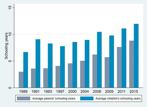
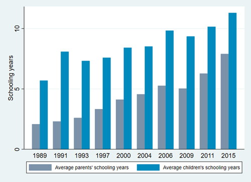
According to the previous definition, the income or years of schooling gap between parents and children denote income upward mobility or education upward mobility. To observe overall income upward mobility and education upward mobility more visual, Figures 1 and 2 compare the average annual income and years of schooling of all parents and children in each cross-section ordered by the year of survey in CHNS, respectively, i.e., average annual income and years of schooling of all parents and children. The bar chart gap between parents and children denote the overall upward mobility in current period. In most years, children have a higher average income and more years of schooling than their parents. It can also be seen that people’s income increases over time, and that in every year children’s income is higher than their parents’ income. The change in the number of people’s years of schooling is similar to the change in people’s income, but the former does not change as rapidly as the latter.

Figure 1. Average annual income of parents and children in general.

Source: drawn by author.

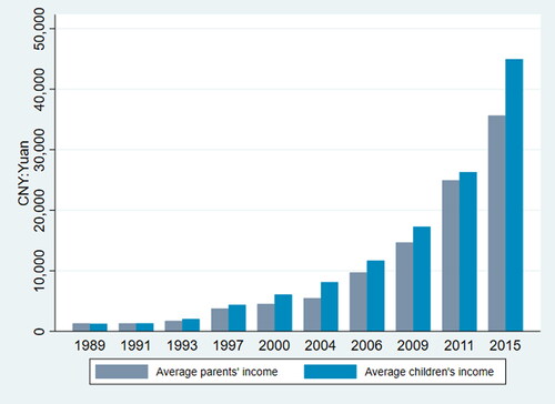
Figure 2. Average annual years of schooling of parents and children in general.

Source: drawn by author.

To analyze the differences between urban and rural areas, we compile an average annual tally of all parents’ and children’s incomes and years of schooling in Figures 3 and 4, respectively, for urban areas, and Figures 5 and 6 for rural areas. It can be seen that the income of urban people increases year-by-year, overall, and that this increase is rapid from 2000 onward. In addition, the difference between parents’ incomes and children’s incomes is not easy to observe for urban-dwellers than for rural-dwellers, and from 1989 to 2015, children’s incomes are similar to their parents’ income in urban areas due to incomes of children and their parents are known to be strongly correlated (Fan et al., 2015; Gong et al., 2012; Yuan, 2017). However, Figure 5 shows that although rural incomes are increasing year-by-year, there is a notable difference between the incomes of parents and children in rural areas, as children earn more than their parents in most years. Figures 4 and 6 show that people’s years of schooling also increase year-by-year, and that the difference between children’s years of schooling and their parents’ years of schooling is greater in rural areas than in urban areas. This is because rural parents have fewer years of schooling than urban parents, and thus rural children are more likely than urban children to exceed their parents’ years of schooling. Finally, children and parents in urban areas have more years of schooling and higher incomes than children and parents in rural areas.

Figure 3. Average annual income of parents and children in urban areas.

Source: drawn by author.

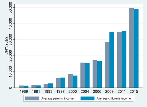
Figure 4. Average annual years of schooling of parents and children in urban areas.

Source: drawn by author.

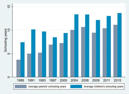
Figure 5. Average annual income of parents and children in rural areas.

Source: drawn by author.

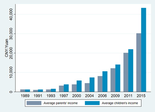
Figure 6. Average annual years of schooling of parents and children in rural areas.

Source: drawn by author.

Most children finish compulsory education, whereas their parents did not, as can be seen in Panel A of Table 1: children have an average of 9.02 years of schooling, whereas parents have an average of 4.95 years of schooling, which is less than the 9 years of education that are compulsory in China. In addition, the preference for sons over daughters persists in China, as shown by the mean of children’s gender being 0.79 which indicates the ratio of female children to male children. Moreover, 31% of parents work in a government agency, state-owned enterprise, or public institution, 7% of parents are cadres, and only 5% of parents have sufficient social capital as the mean of $\mathrm{SOCIAL}$ is 0.05. Finally, the average intergenerational psychological distance (IPD) is 2.33, which means that the age gap between children and parents is a little large because it surpasses level 2 after we divide the IPD into quartiles.

Table 1. Summary statistics.

Variables	Obs.	Mean	Std. Dev.	Min.	Max.
Panel A: Total
${\mathit{INCOME}}^P$	4,032	8,272.01	13,851.87	50	78,000
${\mathit{INCOME}}^C$	4,032	10,459.91	16,880.18	111	92,000
$\mathit{IUM}$	4,032	2,187.91	13,535.53	−74,550	91,400
${\mathit{EDU}}^P$	4,032	4.95	4.54	0	16
${\mathit{EDU}}^C$	4,032	9.02	4.22	0	16
$\mathit{EUM}$	4,032	4.06	4.81	−16	16
${\mathit{AGE}}^P$	4,032	56.06	4.95	43	65
${\mathit{AGE}}^C$	4,032	28.92	3.92	25	45
${\mathit{GENDER}}^C$	4,032	0.79	0.40	0	1
${\mathit{UNIT}}^P$	4,032	0.31	0.46	0	1
${\mathit{CADRE}}^P$	4,032	0.07	0.25	0	1
$\mathit{SOCIAL}$	4,032	0.05	0.22	0	1
$\mathit{IPD}$	4,032	2.33	1.12	1	4
Panel B: Urban
${\mathit{INCOME}}^P$	1,237	10,279.67	16,789.80	50	78,000
${\mathit{INCOME}}^C$	1,237	10,829.77	18,639.96	120	92,000
$\mathit{IUM}$	1,237	550.10	13,185.07	−67,000	91,400
${\mathit{EDU}}^P$	1,237	6.46	5.13	0	15
${\mathit{EDU}}^C$	1,237	10.05	4.92	0	16
$\mathit{EUM}$	1,237	3.59	5.62	−15	16
${\mathit{AGE}}^P$	1,237	56.69	4.79	44	65
${\mathit{AGE}}^C$	1,237	28.69	3.73	25	43
${\mathit{GENDER}}^C$	1,237	0.73	0.44	0	1
${\mathit{UNIT}}^P$	1,237	0.76	0.43	0	1
${\mathit{CADRE}}^P$	1,237	0.13	0.34	0	1
$\mathit{SOCIAL}$	1,237	0.11	0.32	0	1
$\mathit{IPD}$	1,237	2.54	1.12	1	4
Panel C: Rural
${\mathit{INCOME}}^P$	2,795	7,383.46	12,228.84	50	78,000
${\mathit{INCOME}}^C$	2,795	10,296.22	16,040.67	111	92,000
$\mathit{IUM}$	2,795	2,912.76	13,627.38	−74,550	88,840
${\mathit{EDU}}^P$	2,795	4.27	4.06	0	15
${\mathit{EDU}}^C$	2,795	8.56	3.78	0	16
$\mathit{EUM}$	2,795	4.29	4.37	−15	16
${\mathit{AGE}}^P$	2,795	55.79	4.99	43	65
${\mathit{AGE}}^C$	2,795	29.02	3.99	25	45
${\mathit{GENDER}}^C$	2,795	0.82	0.38	0	1
${\mathit{UNIT}}^P$	2,795	0.12	0.32	0	1
${\mathit{CADRE}}^P$	2,795	0.04	0.20	0	1
$\mathit{SOCIAL}$	2,795	0.03	0.16	0	1
$\mathit{IPD}$	2,795	2.24	1.10	1	4

Note: Obs., Mean, Std. Dev., Min., and Max. denote observed value, mean value, standard deviation, minimum value, and maximum value, respectively. ${\mathrm{INCOME}}^{\mathrm{P}},$$\mathrm{ }{\mathrm{INCOME}}^{\mathrm{C}},$ $\mathrm{IUM},$$\mathrm{ }{\mathrm{EDU}}^{\mathrm{P}},$ ${\mathrm{EDU}}^{\mathrm{C}},$ $\mathrm{EUM}$ denote parents’ income, children’s income, income upward mobility, parents’ years of schooling, children’s years of schooling, and education upward mobility, respectively. ${\mathrm{AGE}}^{\mathrm{P}}$ and ${\mathrm{AGE}}^{\mathrm{C}}$ denote the age of parents and children, respectively. ${\mathrm{GENDER}}^{\mathrm{C}}\mathrm{ }$denotes the gender of children. ${\mathrm{UNIT}}^{\mathrm{P}}$ is a dummy variable that is equal to 1 if parents work in a government agency, state-owned enterprise, or public institution, 0 otherwise. ${\mathrm{CADRE}}^{\mathrm{P}}$ is a dummy variable that is equal to 1 if parents are cadres, 0 otherwise. $\mathrm{SOCIAL}$ denotes the social capital of parents, and is a dummy variable that is equal to 1 if parents work in a government agency, state-owned enterprise, and public institution, and are also cadres, 0 otherwise. $\mathrm{IPD}$ denotes intergenerational psychological distance, comprising four levels (increasing from level 1 to 4).

Source: summarized by author.

To clarify the differences between people in urban areas and those in rural areas, we conduct descriptive statistical analyses of the urban and rural samples. Panel B and Panel C in Table 1 show that the children’s average years of schooling in urban and rural areas are 10.05 and 8.56, respectively. Thus, some children in rural areas do not complete their 9 years of compulsory education (as required by the Compulsory Education Law of 1986). Panel B in Table 1 shows that 76% of parents in urban areas work in a government agency, state-owned enterprise, or public institution, compared with only 12% of parents in rural areas. The average value of ${\mathit{CADRE}}^P$ is 0.13 and 0.04 in urban and rural areas, respectively, which shows that more parents in urban areas are cadres than those in rural areas. Finally, the average $\mathrm{IPD}$ is 2.54 in urban areas and 2.24 in rural areas, which shows that the age of childbearing in rural areas is younger than that in urban areas.

According to the above analysis, there are differences between urban and rural areas in terms of people’s income, years of schooling, the intergenerational psychological distance and parents’ social capital. Therefore, in the following section we empirically analyze the urban panel and rural panel separately.

3. Empirical results

3.1. Benchmark analysis

To explore the effect of EUM on IUM, we run the following ordinary least squares (OLS) regression: (4) $${\mathrm{IUM}}_{\mathrm{i}}={\mathrm{\beta }}_0+{\mathrm{\beta }}_1\times {\mathrm{EUM}}_{\mathrm{i}}+\mathrm{\beta }\times {\mathrm{X}}_{\mathrm{i}}+{\mathrm{R}}_{\mathrm{i}}+{\mathrm{Y}}_{\mathrm{t}}+{\mathrm{\epsilon }}_{\mathrm{i}}$$(4) where ${\mathrm{\beta }}_1$ represents the effect of EUM on IUM; $R_i$ and $Y_t$ are year dummies and province dummies, respectively, which filter the effect of year and region; and $X_i$ is a set of control variables (such as parents’ income, children’s age and quadratic, and parents’ age and quadratic). To negate the influence of extreme values on the regression results, we winsorize parents’ income and children’s income at the 1% level. To prevent dimensional inconsistencies, we standardize the EUM, the IUM, and parents’ income in the regression analysis.

As mentioned above, urban and rural areas differ in terms of people’s income (Liu et al., 2013) and educational status (Rao & Ye, 2016), and in terms of development models (Song et al., 2012; Zheng & Yu, 2011). As these differences may affect the relationship between EUM and IUM in our study, we follow Guo et al. (2019) and divide the sample into an urban panel and a rural panel according to people’s type of hukou, and then perform a comparative empirical analysis. The results are shown in Table 2.

Table 2. Effect of education upward mobility (EUM) on income upward mobility (IUM).

Variable	Total	Urban	Rural
	(1)	(2)	(3)
$\mathit{EUM}$	0.087***	0.086***	0.071***
	(0.016)	(0.026)	(0.019)
Constants	−0.374	2.359	−1.152
	(1.764)	(3.785)	(2.068)
Control_X	Yes	Yes	Yes
Year dummies	Yes	Yes	Yes
Regional dummies	Yes	Yes	Yes
Observations	4,032	1,237	2,795
R^2	0.079	0.051	0.115

Note: The dependent variable is income upward mobility.

Control_X is a set of control variables (parents’ income, children’s age and quadratic, and parents’ age and quadratic).

Robust standard errors are given in brackets, where *p < 0.1, **p < 0.05, and ***p < 0.01.

Source: estimated by author.

Table 2 shows that in the urban sample the level of significance of $\mathit{EUM}$ is 1% and the coefficient is 0.086, whereas in the rural sample the level of significance of $\mathit{EUM}$ is 1% and the coefficient is 0.071. This shows that irrespective of people’s hukou, the education upward mobility can promote the income upward mobility. In addition, this effect is more significant in urban areas, as the coefficient of EUM in urban areas (0.086***) is greater than that in rural areas (0.071***). These findings are intriguing, because some scholars believe that educational factors have little effect on intergenerational income mobility (Blanden, 2013; Narayan et al., 2018). In addition, the results in Table 2 show that (a) children’s IUM can be increased (i.e., the magnitude by which their income is greater than that of their parents can be increased); or (b) the magnitude of the difference between the incomes of children and parents can be decreased (if children’s incomes are less than those of their parents) to help children realize income upward mobility, by increasing children’s magnitude of EUM (if children have more years of schooling than their parents) or decreasing the difference between the years of schooling of children and those of their parents (if children have fewer years of schooling than their parents). Thus, in the following analysis, IUM and EUM are always defined in this manner, aside from in Sec. 3.4, where we change the measures of upward mobility to test robustness.

3.2. Effect of IPD

In this section, we consider the effect of the intergenerational psychological distance (IPD) between parents and children, as this leads to parents and children developing different and conflicting conceptualizations, beliefs, and opinions (Carton & Cummings, 2012; De Meulenaere et al., 2016; Gibson & Vermeulen, 2003). Parents’ conceptualizations of career choice may influence their children’s career choice, and thus affect their children’s income. Thus, the magnitude of IPD may influence the effect of EUM on IUM. We therefore perform the following OLS: (5) $${\mathit{IUM}}_i={\beta }_0+{\beta }_1\times {\mathit{IPD}}_j+{\beta }_2\times {\mathit{EUM}}_i\times {\mathit{IPD}}_j+\beta \times X_i+R_i+Y_t+{\epsilon }_i$$(5) where $IP{D}_j$ denotes the age gap between parents and children, i.e., the IPD. We divide ${\mathit{IPD}}_j$ into quartiles to measure it at four levels (Guo et al., 2019) corresponding to four age-ranges: 18–24, 24–27, 27–30, and 30–40 years. ${\beta }_2$ measures the effect of EUM on IUM at these various levels of IPD; $R_i$ and $Y_t$ are year dummies and province dummies, respectively; and $X_i$ is a set of control variables (such as children’s age and quadratic, and parents’ age and quadratic). To examine whether the effects of variations in the levels of IPD differ between urban and rural areas, we run Eq. (5)(5) $${\mathit{IUM}}_i={\beta }_0+{\beta }_1\times {\mathit{IPD}}_j+{\beta }_2\times {\mathit{EUM}}_i\times {\mathit{IPD}}_j+\beta \times X_i+R_i+Y_t+{\epsilon }_i$$(5) using the total sample, the urban sample, and the rural sample, respectively. The results are shown in Table 3.

Table 3. Influence of intergenerational psychological distance (IPD).

Variable	Total	Urban	Rural
	(1)	(2)	(3)
EUM × IPD1	0.130***	0.134***	0.106***
	(0.028)	(0.048)	(0.035)
EUM × IPD2	0.114***	0.137**	0.071*
	(0.035)	(0.060)	(0.041)
EUM × IPD3	0.065**	0.065**	0.059
	(0.026)	(0.033)	(0.039)
EUM × IPD4	0.007	−0.010	0.017
	(0.027)	(0.041)	(0.035)
IPD2	−0.108*	−0.142	−0.078
	(0.059)	(0.122)	(0.068)
IPD3	−0.074	−0.064	−0.072
	(0.075)	(0.153)	(0.085)
IPD4	−0.123	−0.140	−0.101
	(0.117)	(0.217)	(0.134)
Constants	−1.076	1.818	−1.788
	(2.017)	(4.555)	(2.347)
Control_X	Yes	Yes	Yes
Year dummies	Yes	Yes	Yes
Regional dummies	Yes	Yes	Yes
Observations	4,032	1,237	2,795
R^2	0.082	0.059	0.116

Note: The dependent variable is income upward mobility; EUM denotes education upward mobility.

IPD1, IPD2, IPD3, and IPD4 denote four levels of IPD.

Control_X is a set of control variables, such as parents’ income, children’s age and quadratic, and parents’ age and quadratic.

Robust standard errors are in brackets, where *p < 0.1, **p < 0.05, and ***p < 0.01.

Source: estimated by author.

As the first column in Table 3 shows, the levels of significance of EUM × IPD₁, EUM × IPD₂, EUM × IPD₃ are 1%, 1%, 5%, respectively, and the values of their coefficient are 0.130, 0.114, and 0.065, respectively. This shows that the IPD does not change the positive influence of EUM on IUM overall, but that a large IPD can weaken this influence at IPD₄, as EUM × IPD₄ is insignificant. Analogously, low IPD has a directly negative effect on children’s IUM, as the level of significance of IPD₂ is 10% and its coefficient is −0.108. These results show that the effect of EUM on IUM may be negated by a large IPD due to the difference between parents’ and children’s conceptualizations of career choices. Thus, the greater the age gap between parents and children, the greater the IPD, and the more likely there will be conflicts between parents and children regarding their conceptualizations of career choices. For example, in the pre-1990s China, many industries offered low wages, and unemployment was common. Thus, people wished to find a job with high stability, a so-called iron rice-bowl job, typically in a government agency, state-owned enterprise, or public institution. However, during the time interval we use, the average income of these jobs is generally lower than in other intervals according to the average salary statistics from Chinese State Statistical Bureau.⁴ Nevertheless, there is a strong belief in the desirability of iron rice-bowl jobs during this time interval, particularly in families where the IPD is large, and thus parents in such families persuade their children to seek iron rice-bowl jobs. Therefore, these children are more likely to choose jobs with lower incomes but high stability, such that their income is less sensitive to EUM. The regression results from the urban sample and the rural sample suggest that parents’ preference for an iron rice-bowl job has a great influence on the type of job chosen by children in rural areas. This is different from the situation in urban areas, where children can realize IUM by enhancing their EUM at almost every IPD level. This is because in the rural sample, only EUM × IPD₁ and EUM × IPD₂ are significant, whereas in the urban sample, EUM × IPD₁, EUM × IPD₂, and EUM × IPD₃ are significant. Moreover, a lower IPD may have a direct negative effect on IUM by children who have less IPD have more problems in income (Hofferth & Reid, 2002).

3.3. Influence of parents’ social capital

Li et al. (2012) and Yuan and Chen (2013) find that parents’ social capital have a positive effect on children’s incomes. For these children, their incomes may be more sensitive to parents’ social capital rather than education. Thus, it may weaken the impact of EUM on IUM. To examine the effect of parents’ social capital, we run the following OLS regression: (6) $${\mathit{IUMi}}_i={\beta }_0+{\beta }_1\times {\mathit{SOCIAL}}^P+{\beta }_2\times {\mathit{IUM}}_i\times {\mathit{SOCIAL}}^P+\beta \times X_i+R_i+Y_t+{\epsilon }_i$$(6) where ${\mathit{SOCIAL}}^P$ denotes parents’ social capital, and is a dummy variable that is equal to 1 if parents work in a government agency, state-owned enterprise, or public institution, and are also cadres, 0 otherwise.$\mathrm{ }{\mathrm{\beta }}_2$ is a measure of the effect of EUM on IUM that results from different types of parents’ social capital; and $R_i$ and $Y_t$ are year dummies and province dummies, respectively. As social capital has a substantial independent influence on income (Boxman et al., 1991), we add parents’ income as a control variable: thus, $X_i$ includes control variables such as children’s age and quadratic, parents’ age and quadratic, and parents’ income. To determine whether the effects of parents’ social capital on the relationship between EUM and IUM differs by area, we run Eq. (6)(6) $${\mathit{IUMi}}_i={\beta }_0+{\beta }_1\times {\mathit{SOCIAL}}^P+{\beta }_2\times {\mathit{IUM}}_i\times {\mathit{SOCIAL}}^P+\beta \times X_i+R_i+Y_t+{\epsilon }_i$$(6) with the total sample, the urban sample, and the rural sample, separately. The results are shown in Table 4.

Table 4. Influence of parents’ social capital.

Variable	Total	Urban	Rural
	(1)	(2)	(3)
EUM × SOCIAL0	0.045***	0.033	0.060***
	(0.013)	(0.022)	(0.016)
EUM × SOCIAL1	0.063*	0.101***	−0.020
	(0.038)	(0.040)	(0.065)
SOCIAL1	0.085*	0.010	0.167*
	(0.050)	(0.052)	(0.101)
Constants	0.160	3.024	−1.137
	(1.381)	(2.862)	(1.636)
Control_X	Yes	Yes	Yes
Year dummies	Yes	Yes	Yes
Regional dummies	Yes	Yes	Yes
Observations	4,032	1,237	2,795
R^2	0.401	0.390	0.421

Note: The dependent variable is income upward mobility; EUM denotes education upward mobility.

$\mathit{SOCIAL}$ is a dummy variable that is equal to 1 if parents work in a government agency, state-owned enterprise, or public institution, and are also cadres, and 0 otherwise.

Control_X is set of control variables, such as parents’ income, children’s age and quadratic, parents’ age and quadratic, and parents’ income.

Robust standard errors are given in brackets, where *p < 0.1, **p < 0.05, and ***p < 0.01.

Source: estimated by author.

As the first column in Table 4 indicates, parents’ social capital does not influence the positive effect of EUM on IUM in general. That is, children’s education affects their income irrespective of whether their parents have social capital, as shown by the significance levels of EUM × SOCIAL₀ and EUM × SOCIAL₁ being 1% and 10%, respectively. However, parents’ social capital can directly affect IUM, as shown by the significance level of SOCIAL₁ being 10%. This means that children whose parents have social capital can earn more than children whose parents do not have social capital, which is consistent with the results of Batjargal and Liu (2004) and Li et al. (2012). In urban areas, the effect of EUM on IUM is conditional: the second column shows that EUM × SOCIAL₁ is the only significant variable (0.101***), meaning that only children whose parents have social capital can improve their IUM by increasing their EUM, and thus parents’ social capital does not directly affect children’s incomes. This is probably because highly paying urban employers prefer to hire children who have both more education and parents with social capital, rather than children who have either more education or parents with social capital.

In rural areas, we find that IUM is less sensitive to EUM if children have parents with social capital, as shown by the non-significance of EUM × SOCIAL₁ (column 2), and that parents’ social capital has a direct positive effect on children’s IUM, as shown by the level of significance of SOCIAL₁ being 10% and its coefficient being 0.167. This suggests that employers consider children with parents who have social capital to be better employees than children with more years of schooling. This may be because employers believe that the children whose parents have social capital can bring more benefits to a business unit (Montgomery, 1991) than children with more years of schooling. However, children whose parents do not have social capital can nevertheless realize IUM by increasing their EUM.

3.4. Influence of children’s gender

In many developing countries, people prefer sons over daughters (Ebenstein & Leung, 2010); notably, this preference varies by region in China (Li et al., 2019). In addition, there are gender differences in income (Carnevale et al., 2018), education (Hannum et al., 2009), employment status (Goldin & Rouse, 2000), and concerns from parents (Gong et al., 2005; Iddrisu et al., 2018). These differences may weaken the effect of EUM on IUM for girls. Thus, in this section we study the influence of gender heterogeneity more comprehensively, by considering the preference for boys or girls caused by region (Li et al., 2019). That is, we rather than setting regional dummies as is done previously. Thus, we run Eqs. (4)–(6) by OLS without setting regional dummies on different samples from urban and rural areas sorted by children’s gender. The results are shown in Table 5. It reveals that in the total sample, the positive effect of EUM on IUM is not affected by children’s gender, as EUM (0.089***) and EUM (0.081**) in column 1 and column 2, respectively. There are similar results in the urban sample. However, rural girls benefit less from education than rural boys, as the EUM in column 6 is insignificant. This result does not contradict our main conclusion, as the positive effect of EUM (0.088***) on IUM persists in rural areas in column 5. We clarify the effect of children’s gender on EUM and IUM in further discussions below.

Table 5. Analysis of gender heterogeneity via basic regression.

Variable	Total		Urban		Rural
	Son	Daughter	Son	Daughter	Son	Daughter
	(1)	(2)	(3)	(4)	(5)	(6)
EUM	0.089***	0.081**	0.079***	0.120**	0.088***	0.032
	(0.017)	(0.034)	(0.025)	(0.052)	(0.022)	(0.042)
Constants	−0.399	−0.591	−2.431	14.175	−0.041	−7.180*
	(1.817)	(4.636)	(3.236)	(10.339)	(2.244)	(3.986)
Control_X	Yes	Yes	Yes	Yes	Yes	Yes
Year dummies	Yes	Yes	Yes	Yes	Yes	Yes
Observations	3,200	832	904	333	2,296	499
R^2	0.081	0.071	0.034	0.082	0.115	0.108

Note: The dependent variable is income upward mobility; EUM denotes education upward mobility.

Control_X is a set of control variables, such as parents’ income, children’s age and quadratic, and parents’ age and quadratic.

Robust standard errors are given in brackets, where *p < 0.1, **p < 0.05, and ***p < 0.01.

Source: estimated by author.

Table 6 reveals that parents’ conceptualization of job choice, which results from IPD, has a greater influence on daughters than on sons, as daughters barely benefit from EUM at different levels of IPD, whereas this is not true for sons. In many countries and regions, people believe that daughters should not receive much education, and should instead be full-time housewives or have easy jobs with short working hours when they come of age, such that they have more time to take care of their families (Fincher, 2016; Li et al., 2019). This means that in these areas daughters typically receive less education and have fewer employment opportunities than sons, and are thus less sensitive to EUM. Furthermore, the results in column 6 show that IPD has a direct negative effect on the IUM of rural daughters, as the level of significance of IPD₂ is 5% and the coefficient is −0.365; notably, this effect is so strong that the total sample also shows a similar result. Thus, taken together with the research of Hofferth and Reid (2002), we conclude that the direct negative effect of IPD on children’s income is not universal, as it is more pronounced for rural daughters than for rural sons.

Table 6. Analysis of gender heterogeneity of influence of intergenerational psychological distance (IPD).

Variable	Total		Urban		Rural
	Son	Daughter	Son	Daughter	Son	Daughter
	(1)	(2)	(3)	(4)	(5)	(6)
EUM × IPD1	0.143***	0.084*	0.139**	0.260**	0.135***	−0.008
	(0.033)	(0.049)	(0.056)	(0.115)	(0.041)	(0.056)
EUM × IPD2	0.103***	0.146*	0.111**	0.220	0.084*	0.084
	(0.034)	(0.084)	(0.048)	(0.151)	(0.048)	(0.081)
EUM × IPD3	0.075**	0.062	0.052	0.092	0.085**	−0.007
	(0.030)	(0.052)	(0.042)	(0.058)	(0.039)	(0.125)
EUM × IPD4	−0.001	−0.011	−0.009	−0.060	0.013	0.034
	(0.033)	(0.041)	(0.054)	(0.052)	(0.043)	(0.065)
IPD2	−0.036	−0.301**	−0.114	−0.147	−0.001	−0.365**
	(0.066)	(0.137)	(0.136)	(0.291)	(0.076)	(0.145)
IPD3	−0.047	−0.077	−0.136	0.258	−0.013	−0.280
	(0.084)	(0.195)	(0.162)	(0.401)	(0.097)	(0.214)
IPD4	−0.036	−0.362	−0.175	−0.082	0.013	−0.501*
	(0.133)	(0.263)	(0.234)	(0.510)	(0.155)	(0.291)
Constants	−0.732	−1.594	−3.495	20.839	−0.053	−11.531**
	(2.028)	(6.230)	(3.834)	(13.018)	(2.489)	(5.222)
Control_X	Yes	Yes	Yes	Yes	Yes	Yes
Year dummies	Yes	Yes	Yes	Yes	Yes	Yes
Observations	3,200	832	904	333	2,296	499
R^2	0.083	0.089	0.039	0.125	0.116	0.123

Note: The dependent variable is income upward mobility; EUM denotes education upward mobility.

IPD1, IPD 2, IPD3, and IPD 4 denote four levels of IPD.

Control_X is a set of control variables, such as parents’ income, children’s age and quadratic, and parents’ age and quadratic.

Robust standard errors are given in brackets, where *p < 0.1, **p < 0.05, and ***p < 0.01.

Source: estimated by author.

Ultimately, we find that sons benefit more from parents’ social capital than daughters. As column 1 in Table 7 shows, parents’ social capital directly promotes sons’ IUM in general (as the level of significance of SOCIAL₁ is 5% and the coefficient is 0.117), and sons whose parents do not have social capital can improve their IUM by increasing their EUM (as the level of significance of EUM × SOCIAL₀ is 1% and the coefficient is 0.066). In contrast, daughters’ IUM is less sensitive to parents’ social capital or EUM, as EUM × SOCIAL₀, EUM × SOCIAL₁, and SOCIAL₁ are insignificant in column 2, column 4, and column 6. This is most likely due to employers preferring to hire boys rather than girls. Thus, even if girls receive more education or their parents have social capital, they are less likely to be hired than boys, and thus are more likely to fail to realize IUM. In addition, the results for the urban son sample and rural son sample are the same as those for the urban and rural samples in Table 4, which underscores the dominance of sons in these samples.

Table 7. Analysis of effect of gender heterogeneity on the influence of parents’ social capital.

Variable	Total		Urban		Rural
	Son	Daughter	Son	Daughter	Son	Daughter
	(1)	(2)	(3)	(4)	(5)	(6)
EUM × SOCIAL0	0.066***	0.033	0.033	0.075	0.088***	0.038
	(0.015)	(0.029)	(0.022)	(0.052)	(0.019)	(0.028)
EUM × SOCIAL1	0.062	0.045	0.130**	0.054	−0.045	−0.026
	(0.060)	(0.049)	(0.058)	(0.071)	(0.098)	(0.073)
SOCIAL1	0.117**	−0.001	0.024	−0.171	0.238*	0.095
	(0.059)	(0.132)	(0.061)	(0.203)	(0.136)	(0.199)
Constants	−1.479	−0.289	−3.981	13.203	−1.204	−5.577*
	(1.418)	(4.107)	(2.562)	(8.837)	(1.790)	(2.859)
Control_X	Yes	Yes	Yes	Yes	Yes	Yes
Year dummies	Yes	Yes	Yes	Yes	Yes	Yes
Observations	3,200	832	904	333	2,296	499
R^2	0.373	0.340	0.407	0.265	0.380	0.513

Note: The dependent variable is income upward mobility; EUM denotes education upward mobility.

$\mathit{SOCIAL}$ is a dummy variable that is equal to 1 if parents work in a government agency, state-owned enterprise, or public institution, and are also cadres, and 0 otherwise.

Control_X is a set of control variables, such as parents’ income, children’s age and quadratic, parents’ age and quadratic, and parents’ income.

Robust standard errors are given in brackets, where *p < 0.1, **p < 0.05, and ***p < 0.01.

Source: estimated by author.

4. Robustness checks

4.1. Alternative measurement

We adopt a new measurement of upward mobility, which reveals the presence and the extent of upward mobility (or the gap between children and parents) by accurately calculating the difference between children’s and parents’ years of schooling or income. This provides a basis for further study of the effect of EUM on IUM. We also use measurements from other studies for robustness checks. Thus, with reference to Checchi et al. (1999) and Majumder (2010), we measure upward mobility using a dummy variable that is equal to 1 if children surpass their parents in specific factors, 0 otherwise, and run the following logistic regression: (7) $${\mathit{INC}}_{c>p}={\beta }_0+{\beta }_1\times {\mathit{EDU}}_{c>p}+\beta \times X_i+R_i+Y_t+{\epsilon }_i$$(7) where ${\beta }_1$ is the odds ratio of the effect of EUM on IUM; ${\mathit{INC}}_{c>p}$ is a dummy variable that is equal to 1 if children’s income is higher than their parents’ income, and 0 otherwise; ${\mathit{EDU}}_{c>p}$ is a dummy variable that is equal to 1 if children’s years of schooling are greater than their parents’ years of schooling; $R_i$ and $Y_t$ are year dummies and province dummies, respectively; and $X_i$ is a set of control variables, such as children’s age and quadratic, and parents’ age and quadratic. As column 1 in Table 8 shows, EUM increases the probability of children realizing IUM in general (as the level of significance of EDU is 1% and the odds ratio is 1.666). In addition, the results for the urban and rural samples are consistent with the results for the total sample. In urban areas, the level of significance of EDU is 1% and its odds ratio is 1.840 (column 2); similarly, in rural areas, the significance level of EDU is 1% and the odds ratio is 1.512 (column 3). This shows that education is critical for raising children’s income, which supports our previous results.

Table 8. Robustness check using alternative measurements.

Variable	Total	Urban	Rural
	(1)	(2)	(3)
EDU	1.666***	1.840***	1.512***
	(0.127)	(0.264)	(0.142)
Log-likelihood	−2,681.83	−776.36	−1,847.20
Control_X	Yes	Yes	Yes
Year dummies	Yes	Yes	Yes
Regional dummies	Yes	Yes	Yes
Observations	4,032	1,237	2,795
Pseudo R^2	0.038	0.087	0.035

Note: The dependent variable is income upward mobility, and the independent variable is education upward mobility. Both are dummy variables that equal 1 if children surpass their parents’ income and education, and 0 otherwise.

Control_X is a set of control variables, such as parents’ income, children’s age and quadratic, and parents’ age and quadratic.

Robust standard errors are given in brackets, where *p < 0.1, **p < 0.05, and ***p < 0.01.

Source: estimated by author.

4.2. Potential endogeneity

Children’s personal ability may affect the values of the independent variables and dependent variables. That is, the greater the personal ability that children have, the higher the probability they have a high income and many years of schooling, which may cause endogeneity. Thus, we assume that children’s personal ability is an endogenous factor, and use the Compulsory Education Law (CPL) as an instrumental variable in our regression to provide more support for our results. CPL is a dummy variable that is equal to 1 if children are born after 1980 and do not go to college, 0 otherwise. The Compulsory Education Law enacted in China in 1986 stipulates that children must receive education from the age of 6 years; thus, children born after 1980 are 6 years old in 1986, and therefore meet the condition to receive compulsory education. As the Compulsory Education Law is not selective, i.e., is not affected by differences in children’s personal abilities, its enaction increases all children’s years of schooling and has positive contributions to EUM. In addition, we filter the effect of personal ability in terms of whether children go to university, as university education is not basic education and admits only a fraction of children through entrance examinations. It follows that children who go to university are more likely to have personal ability that may influence their income than children who do not go to university. Thus, CPL is a suitable instrumental variable, as it is related directly to the independent variable, but not to the dependent variable.

We run Eq. (3)(3) $${\mathit{IPD}}_i={\mathit{AGE}}_i^P-{\mathit{AGE}}_i^C$$(3) using a two-stage least squares method, with CPL as the instrumental variable, and the results are given in Table 9. As can be seen, the level of significance of CPL is 5%, 10%, and 1% and the coefficient is 0.520, 0.514, and 0.771 in the total sample, urban areas, and rural areas, respectively. This means providing children with more education increases their IUM, irrespective of their personal ability and hukou. These results are consistent with our main conclusion. Thus, children’s personal ability does not affect our conclusions, and our previous conclusions are robust.

Table 9. Robustness check using an instrumental variable.

Variable	Total	Urban	Rural
	(1)	(2)	(3)
CPL	0.520**	0.514*	0.771***
	(0.220)	(0.281)	(0.261)
Constants	−0.767	4.236	−2.604
	(1.903)	(4.231)	(2.499)
Control_X	Yes	Yes	Yes
Year dummies	Yes	Yes	Yes
Regional dummies	Yes	Yes	Yes
Observations	4,032	1,237	2,795

Note: The dependent variable is income upward mobility.

CPL is a dummy variable that is equal to 1 if children are born after the Compulsory Education Law was enacted in China and do not go to college, and 0 otherwise.

Control_X is a set of control variables, such as parents’ income, children’s age and quadratic, and parents’ age and quadratic.

Robust standard errors are given in brackets, where *p < 0.1, **p < 0.05, and ***p < 0.01.

Source: estimated by author.

4.3. Subsample regression

In 1999, China implemented its college expansion policy, which enabled many more children to go to college. This may render years of schooling less valuable and affect the relationship between EUM and IUM. To determine whether this policy affects our previous results, we exclude samples from years before 2003 (as this was the first post-policy year in which college students graduated and were employed), and run an OLS (Eq. (3)(3) $${\mathit{IPD}}_i={\mathit{AGE}}_i^P-{\mathit{AGE}}_i^C$$(3) ) on the resulting subsample. The results are presented in Table 10, and show that in the urban sample the level of significance of $\mathrm{EUM}$ is 1% and the coefficient is 0.086, whereas in the rural sample the level of significance of EUM is 1% and the coefficient is 0.071. Thus, we find that EUM has a significant effect on IUM that is independent of the influence of the college expansion policy, and that this effect is more significant in urban areas than in rural areas. Thus, our results are robust.

Table 10. Robustness check on subsample: influence of college expansion policy.

Variable	Total	Urban	Rural
	(1)	(2)	(3)
EUM	0.197***	0.309***	0.124**
	(0.046)	(0.106)	(0.049)
Constants	−5.712	−0.876	−8.038
	(5.448)	(14.611)	(5.901)
Control_X	Yes	Yes	Yes
Year dummies	Yes	Yes	Yes
Regional dummies	Yes	Yes	Yes
Observations	1,472	325	1,147
R^2	0.071	0.110	0.100

Note: The dependent variable is income upward mobility; EUM denotes education upward mobility.

Control_X is a set of control variables, such as parents’ income, children’s age and quadratic, and parents’ age and quadratic.

Robust standard errors are given in brackets, where *p < 0.1, **p < 0.05, and ***p < 0.01.

Source: estimated by author.

5. Conclusion

In this paper, we use 10 waves of CHNS data to study the direct effect of EUM on IUM, to determine whether more years of schooling can increase children’s income. We do so by considering China’s unique hukou system and studying upward mobility in an urban panel and a rural panel. We comparatively analyze these two panels and perform study of the effect of IPD on IUM, and also analyze the effects of parents’ social capital and children’s gender. Furthermore, we conduct a series of robustness checks to provide more support for our research results.

We draw some important conclusions from this empirical research. First, we provide evidence that EUM generally has a positive effect on IUM in urban and rural areas. Second, the magnitude of IPD has a differential influence on this relationship. Specifically, a certain magnitude of IPD strengthens the positive effect of EUM on IUM, but an excessive magnitude of IPD negates the positive effect of EUM on IUM, and this influence is more prevalent in rural areas. In addition, as EUM actively promotes the IUM of children from rural families whose parents lack social capital, i.e., education is an important factor for increasing the income of these children. In contrast, in urban areas, only children whose parents have social capital can improve their IUM by increasing their EUM. Therefore, more attention should be paid to the effect of urban children’s education on their income, to weaken the link between parents’ social capital and their children’s income in urban areas. In addition, we find that girls are more likely to be overlooked by employers, irrespective of their educational level. This demonstrates that more research must be performed on the relationship between girls’ incomes, education, and employment status, to improve girls’ opportunities for improved incomes.

The results of the paper may have useful policy implications. For example, governments may be concerned about whether increasing children’s education could increase national income levels. This paper shows that EUM generally has a positive effect on IUM in urban and rural areas. National income levels will increase as each generation experiences income upward mobility. Governments may strengthen the positive effect by appealing to reduce the intervention to children’s career choice, putting an end to the link between parents’ social capital and their children’s chance to get job and introducing more polices to guarantee female employees will not be overlooked.

We acknowledge three main limitations in the present study. First, though we invest a lot of work in database selection and data processing to ensure the quality of the data and the enough number of research samples, the potential for unidentified biases remains. Second, our data is pooled cross-sectional. Thus, our findings cannot be interpreted as evidence of underlying causal relationships, but providing more evidences to prior proven causal relationships. Third, we only research samples from China. Therefore, our findings may not be applicable to all countries due to different social system.

To research the relationship between EUM and IUM more comprehensively, we consider the effect of gender heterogeneity. In future research, this paper has several potential directions. For example, in this paper, we only research the effect gender heterogeneity on the relationship between EUM and IUM. The governments may concern more to the causes of this heterogeneity, i.e., the reasons why females are overlooked. It will help governments introduce more detailed policies to strengthen the positive effect of EUM on IUM. In addition, according to the previous section, scholars have been demonstrated that gender preference varies by region in China. Beyond that, this paper shows that girls are more likely to be overlooked by employers, and it will weaken the positive effect of EUM on IUM. Therefore, further research on gender preferences arising from regional differences may provide more ideas for studying on the inequality of regional economic development.

Disclosure statement

The authors declare that they have no conflict of interest.

Notes

1 The maximum retirement age is 65 in China. According to China's legal rules, the employment contract terminates when the employee gets retired. The retired employee can no longer be protected by the provisions on Minimum Wage and the sum of wages shall be freely concluded by both parties. Thus, we exclude samples older than 65 years due to these people’s wage may deviate from labor market prices and it may mislead our research. Source: http://www.mohrss.gov.cn/ldgxs/LDGXzhengcefagui/LDGXzyzc/201011/t20101116_86291.html.

2 According to the codebook of CHNS, total net individual income sums individual’s income from all sources. Source: https://www.cpc.unc.edu/projects/china/data/datasets/Individual%20Income%20Variable%20Construction.pdf.

3 CHNS doesn't contain individual's years of schooling but record individual's education level. I convert individual's education level to individual's years of schooling according to China's education policy. Source: http://www.moe.gov.cn/jyb_xxgk/xxgk_jyta/jyta_zgs/201902/t20190220_370429.html.

4 https://data.stats.gov.cn/

References

- Acs, G., Elliott, D., & Kalish, E. (2016). What would substantially increased mobility from poverty look like. US Partnership on Mobility from Poverty Working Paper. Urban Institute, Washington, DC. https://www.urban.org/sites/default/files/publication/82811/2000871-What-Would-Substantially-Increased-Mobility-from-Poverty-Look-Like.pdf
- Batjargal, B., & Liu, M. (2004). Entrepreneurs’ access to private equity in China: The role of social capital. Organization Science, 15(2), 159–172. https://doi.org/10.1287/orsc.1030.0044
- Becker, G. S., & Tomes, N. (1979). An equilibrium theory of the distribution of income and intergenerational mobility. Journal of Political Economy, 87(6), 1153–1189. https://doi.org/10.1086/260831
- Björklund, A. (1993). A comparison between actual distributions of annual and lifetime income: Sweden 1951–89. Review of Income and Wealth, 39(4), 377–386.
- Blanden, J. (2013). Cross‐country rankings in intergenerational mobility: A comparison of approaches from economics and sociology. Journal of Economic Surveys, 27(1), 38–73. https://doi.org/10.1111/j.1467-6419.2011.00690.x
- Blanden, J., & Machin, S. (2013). Educational inequality and the expansion of UK higher education. Scottish Journal of Political Economy, 60(5), 578–596. https://doi.org/10.1111/sjpe.12024
- Blomstrom, M., Lipsey, R. E., & Zejan, M. (1992). What explains developing country growth? NBER working paper (w4132).
- Bowles, S., & Gintis, H. (2002). Schooling in capitalist America revisited. Sociology of Education, 75(1), 1–18. https://doi.org/10.2307/3090251
- Boxman, E. A., De Graaf, P. M., & Flap, H. D. (1991). The impact of social and human capital on the income attainment of Dutch managers. Social Networks, 13(1), 51–73. https://doi.org/10.1016/0378-8733(91)90013-J
- Carnevale, A. P., Smith, N., & Gulish, A. (2018). Women can’t win: Despite making educational gains and pursuing high-wage majors, women still earn less than men. Retrieved from Georgetown University, Center on Education. https://cew.georgetown.edu/cew-reports/genderwagegap/#full-report.
- Carton, A. M., & Cummings, J. N. (2012). A theory of subgroups in work teams. Academy of Management Review, 37(3), 441–470. https://doi.org/10.5465/amr.2009.0322
- Checchi, D., Ichino, A., & Rustichini, A. (1999). More equal but less mobile?: Education financing and intergenerational mobility in Italy and in the US. Journal of Public Economics, 74(3), 351–393. https://doi.org/10.1016/S0047-2727(99)00040-7
- Chetty, R., Grusky, D., Hell, M., Hendren, N., Manduca, R., & Narang, J. (2017). The fading American dream: Trends in absolute income mobility since 1940. Science (New York, NY), 356(6336), 398–406. https://doi.org/10.1126/science.aal4617
- Chetty, R., Hendren, N., Jones, M. R., & Porter, S. R. (2020). Race and economic opportunity in the United States: An intergenerational perspective. The Quarterly Journal of Economics, 135(2), 711–783. https://doi.org/10.1093/qje/qjz042
- Chetty, R., Hendren, N., Kline, P., & Saez, E. (2014). Where is the land of opportunity? The geography of intergenerational mobility in the United States. The Quarterly Journal of Economics, 129(4), 1553–1623. https://doi.org/10.1093/qje/qju022
- Coady, D., & Dizioli, A. (2018). Income inequality and education revisited: Persistence, endogeneity and heterogeneity. Applied Economics, 50(25), 2747–2761. https://doi.org/10.1080/00036846.2017.1406659
- Cole, E. R., & Omari, S. R. (2003). Race, class and the dilemmas of upward mobility for African Americans. Journal of Social Issues, 59(4), 785–802. https://doi.org/10.1046/j.0022-4537.2003.00090.x
- Darku, A. B., & Yeboah, R. (2018). Economic openness and income growth in developing countries: A regional comparative analysis. Applied Economics, 50(8), 855–869. https://doi.org/10.1080/00036846.2017.1343449
- De Meulenaere, K., Boone, C., & Buyl, T. (2016). Unraveling the impact of workforce age diversity on labor productivity: The moderating role of firm size and job security. Journal of Organizational Behavior, 37(2), 193–212. https://doi.org/10.1002/job.2036
- Ebenstein, A., & Leung, S. (2010). Son preference and access to social insurance: Evidence from China’s rural pension program. Population and Development Review, 36(1), 47–70. https://doi.org/10.1111/j.1728-4457.2010.00317.x
- Égert, B., Botev, J., & Turner, D. (2020). The contribution of human capital and its policies to per capita income in Europe and the OECD. European Economic Review, 129, 103560. https://doi.org/10.1016/j.euroecorev.2020.103560
- Eryong, X., & Xiuping, Z. (2018). Education and anti-poverty: Policy theory and strategy of poverty alleviation through education in China. Educational Philosophy and Theory, 50(12), 1101–1112. https://doi.org/10.1080/00131857.2018.1438889
- Fan, Y. (2016). Intergenerational income persistence and transmission mechanism: Evidence from urban China. China Economic Review, 41, 299–314. https://doi.org/10.1016/j.chieco.2016.10.005
- Fan, Y., Yi, J., & Zhang, J. (2015). The Great Gatsby Curve in China: Cross-sectional inequality and intergenerational mobility [Working paper]. CUHK, Hongkong.
- Fincher, L. H. (2016). Leftover women: The resurgence of gender inequality in China. Zed Books Ltd.
- Gang, I. N., Landon-Lane, J. S., & Yun, M.-S. (2002). Gender differences in German upward income mobility. Schmollers Jahrbuch: Journal of Applied Social Science Studies/Zeitschrift Für Wirtschafts-Und Sozialwissenschaften, 123(1), 3–14. https://www.econstor.eu/bitstream/10419/21348/1/dp580.pdf
- Gibson, C., & Vermeulen, F. (2003). A healthy divide: Subgroups as a stimulus for team learning behavior. Administrative Science Quarterly, 48(2), 202–239. https://doi.org/10.2307/3556657
- Goldin, C., & Rouse, C. (2000). Orchestrating impartiality: The impact of “blind” auditions on female musicians. American Economic Review, 90(4), 715–741. https://doi.org/10.1257/aer.90.4.715
- Gong, H., Leigh, A., & Meng, X. (2012). Intergenerational income mobility in urban China. Review of Income and Wealth, 58(3), 481–503. https://doi.org/10.1111/j.1475-4991.2012.00495.x
- Gong, X., Van Soest, A., & Zhang, P. (2005). The effects of the gender of children on expenditure patterns in rural China: A semiparametric analysis. Journal of Applied Econometrics, 20(4), 509–527. https://doi.org/10.1002/jae.780
- Guo, C., & Min, W. (2008). Education and intergenerational income mobility in urban China. Frontiers of Education in China, 3(1), 22–44. https://doi.org/10.1007/s11516-008-0002-x
- Guo, Y., Song, Y., & Chen, Q. (2019). Impacts of education policies on intergenerational education mobility in China. China Economic Review, 55, 124–142. https://doi.org/10.1016/j.chieco.2019.03.011
- Hannum, E., Kong, P., & Zhang, Y. (2009). Family sources of educational gender inequality in rural China: A critical assessment. International Journal of Educational Development, 29(5), 474–486.
- Hofferth, S. L., & Reid, L. (2002). Early childbearing and children’s achievement and behavior over time. Perspectives on Sexual and Reproductive Health, 34(1), 41–49. https://doi.org/10.2307/3030231
- Holcombe, R. G., & Lacombe, D. J. (2004). The effect of state income taxation on per capita income growth. Public Finance Review, 32(3), 292–312. https://doi.org/10.1177/1091142104264303
- Iddrisu, A. M., Danquah, M., Quartey, P., & Ohemeng, W. (2018). Gender bias in households’ educational expenditures: Does the stage of schooling matter? World Development Perspectives, 10, 15–23.
- Isaacs, J. B., Sawhill, I. V., & Haskins, R. (2008). Getting ahead or losing ground: Economic mobility in America. Brookings Institution.
- Islam, S. (1996). Economic freedom, per capita income and economic growth. Applied Economics Letters, 3(9), 595–597. https://doi.org/10.1080/135048596356032
- Jolliffe, D. (2002). Whose education matters in the determination of household income? Evidence from a developing country. Economic Development and Cultural Change, 50(2), 287–312. https://doi.org/10.1086/322880
- Kearney, M. S., & Levine, P. B. (2014). Income inequality, social mobility, and the decision to drop out of high school (No. w20195). National Bureau of Economic Research.
- Lefgren, L., Sims, D., & Lindquist, M. J. (2012). Rich dad, smart dad: Decomposing the intergenerational transmission of income. Journal of Political Economy, 120(2), 268–303. https://doi.org/10.1086/666590
- Li, H., Meng, L., Shi, X., & Wu, B. (2012). Does having a cadre parent pay? Evidence from the first job offers of Chinese college graduates. Journal of Development Economics, 99(2), 513–520. https://doi.org/10.1016/j.jdeveco.2012.06.005
- Li, J., Zhang, J., Zhang, D., & Ji, Q. (2019). Does gender inequality affect household green consumption behaviour in China? Energy Policy, 135, 111071. https://doi.org/10.1016/j.enpol.2019.111071
- Liu, M., Feng, X., Wang, S., & Qiu, H. (2020). China’s poverty alleviation over the last 40 years: Successes and challenges. Australian Journal of Agricultural and Resource Economics, 64(1), 209–228. https://doi.org/10.1111/1467-8489.12353
- Liu, Y., Lu, S., & Chen, Y. (2013). Spatio-temporal change of urban–rural equalized development patterns in China and its driving factors. Journal of Rural Studies, 32, 320–330. https://doi.org/10.1016/j.jrurstud.2013.08.004
- Liu, Z. (2005). Institution and inequality: The hukou system in China. Journal of Comparative Economics, 33(1), 133–157. https://doi.org/10.1016/j.jce.2004.11.001
- Majumder, R. (2010). Intergenerational mobility in educational and occupational attainment: A comparative study of social classes in India. Margin: The Journal of Applied Economic Research, 4(4), 463–494. https://doi.org/10.1177/097380101000400404
- Mincer, J. (1974). Schooling, Experience, and Earnings. Human Behavior & Social Institutions (No. 2). Columbia University Press.
- Montgomery, J. D. (1991). Social networks and labor-market outcomes: Toward an economic analysis. The American Economic Review, 81(5), 1408–1418.
- Narayan, A., Van der Weide, R., Cojocaru, A., Lakner, C., Redaelli, S., Mahler, D. G., … Thewissen, S. (2018). Fair progress? Economic mobility across generations around the world. World Bank Publications.
- Palomino, J. C., Marrero, G. A., & Rodríguez, J. G. (2018). One size doesn’t fit all: A quantile analysis of intergenerational income mobility in the US (1980–2010). The Journal of Economic Inequality, 16(3), 347–367. https://doi.org/10.1007/s10888-017-9372-8
- Pekkarinen, T., Uusitalo, R., & Kerr, S. (2009). School tracking and intergenerational income mobility: Evidence from the Finnish comprehensive school reform. Journal of Public Economics, 93(7–8), 965–973. https://doi.org/10.1016/j.jpubeco.2009.04.006
- Rao, J., & Ye, J. (2016). From a virtuous cycle of rural-urban education to urban-oriented rural basic education in China: An explanation of the failure of China’s Rural School Mapping Adjustment policy. Journal of Rural Studies, 47, 601–611. https://doi.org/10.1016/j.jrurstud.2016.07.005
- Solon, G. (1992). Intergenerational income mobility in the United States. The American Economic Review, 82(3), 393–408. http://www.jstor.org/stable/2117312
- Solon, G. (1999). Intergenerational mobility in the labor market. Handbook of Labor Economics, 3, 1761–1800. https://doi.org/10.1016/S1573-4463(99)03010-2
- Song, H., Thisse, J. F., & Zhu, X. (2012). Urbanization and/or rural industrialization in China. Regional Science and Urban Economics, 42(1–2), 126–134. https://doi.org/10.1016/j.regsciurbeco.2011.08.003
- Sturgis, P., & Buscha, F. (2015). Increasing Inter‐generational social mobility: Is educational expansion the answer? The British Journal of Sociology, 66(3), 512–533.
- Thurow, L. C. (1970). Analyzing the American income distribution. The American Economic Review, 60(2), 261–269.
- Urahn, S. K., Currier, E., Elliott, D., Wechsler, L., Wilson, D., & Colbert, D. (2012). Pursuing the American dream: Economic mobility across generations. Economic Mobility Project Research Report, 2012.
- Wang, S., Yu, X., Zhang, K., Pei, J., Rokpelnis, K., & Wang, X. (2022). How does education affect intergenerational income mobility in Chinese society? Review of Development Economics, 26(2), 774–792. https://doi.org/10.1111/rode.12863
- Yang, J., & Qiu, M. (2016). The impact of education on income inequality and intergenerational mobility. China Economic Review, 37, 110–125. https://doi.org/10.1016/j.chieco.2015.12.009
- Yuan, W. (2017). The sins of the fathers: Intergenerational income mobility in China. Review of Income and Wealth, 63(2), 219–233. https://doi.org/10.1111/roiw.12222
- Yuan, Z., & Chen, L. (2013). The trend and mechanism of intergenerational income mobility in China: An analysis from the perspective of human capital, social capital and wealth. The World Economy, 36(7), 880–898. https://doi.org/10.1111/twec.12043
- Zheng, Z., & Yu, G. (2011). Study on the mechanism evolution of China’s Urban_rural integration development planning and its land system in practice. Energy Procedia, 5, 1852–1858. https://doi.org/10.1016/j.egypro.2011.03.316