Regional aggregate indicators under subnational heterogeneity: evidence from the COVID-19 pandemic in Spain

Abstract

The COVID-19 outbreak forced governments to implement regional measures avoiding the spread of the virus, while evaluating their economic effects. However, official Spanish regional economic information is scarce. We estimate monthly regional aggregated indicators for each Spanish region combining a mixed frequency Dynamic Factor Model with a recursive procedure that identifies the most informative variables capturing economic developments in each region. The set of variables that better describe aggregate economic conditions varies considerably across the regions, which emphasizes the heterogeneity in their productive structures. Our results suggest that the post-pandemic recovery will be uneven across territories, stressing the need to monitor regional economic developments.

Keywords:

• Regional heterogeneity
• aggregate indicators
• factor model
• variable selection
• asymmetric shocks
• synchronization

JEL CLASSIFICATION CODES:

• C32
• C53
• E32
• R11

1. Introduction

The recent COVID-19 outbreak is having important consequences worldwide. This paper focuses on measuring its economic consequences in Spain, where the first stage of the pandemic has been particularly severe. By the 30th of June of 2020, the cumulative confirmed COVID-19 cases per million people in Spain were almost two times greater than in the European Union, 5,331.45 and 2,871.77 respectively. The actual number of cases at that moment could have been even estimated much higher given the limited testing (Ritchie et al., 2020). From mid-March to the end of June of 2020, the Spanish government declared a state of emergency, with a lockdown that restricted people’s mobility and forced Spanish citizens to stay at home. During this period the Spanish government decided on the actions to be implemented nationwide and most economic activity was paralyzed. After the emergency period, each region was given the responsibility to monitor the evolution of the pandemic and the authority for imposing restrictive measures if necessary.

In such a context, there is a special need to measure regional economic developments at a high frequency, not only because the measures to stop the spread of COVID-19 have been implemented on a weekly or biweekly basis (Prieto, 2020); but also because of the fast changes in pandemic evolution.¹ However, aggregate indicators for evaluating the general economic developments, such as Gross Domestic Product (GDP), are released at a low frequency and they are usually published with considerable delay. In Spain, regional GDP for each administrative division is released by the National Institute of Statistics (INE) on an annual basis and with almost a one-year delay. Therefore, the official aggregated information about regional economic evolution during the first stage of the pandemic in 2020 will be released by the end of 2021. For these reasons, the provision of high-frequency regional economic measurements to policymakers and economic agents can certainly improve their decision-making process.

For the early assessment of the economic developments, a disaggregate economic indicator can be used, such as the Industrial Production Index (IPI), which is available at a high frequency and published with short delay. However, IPI only provides a partial measurement of the regional economic activity. Furthermore, the weight of each productive sector varies significantly across the Spanish administrative divisions. The latest available information indicates that Madrid is the region in which production contributes to the total national production the most, while Melilla’s production does at least. Furthermore, the share of the industrial sector in Melilla is 4.3%, while it is more than twice in Madrid, 9.2% (INE, 2019). Thus, comparing disaggregated indicators (i.e. IPI) across regions may provide misleading conclusions due to differences in their economic structures. The aim of this paper is to overcome these limitations in the provision of regional economic information by estimating indicators of the regional aggregate economic performance, conditional on the regional heterogeneity across the Spanish administrative divisions and use them to analyse the economic consequences of the COVID-19 pandemic.

Previous studies have addressed the estimation of aggregate indicators that summarize national economic activity by means of Dynamic Factor Models (DFM). Stock and Watson (1991) use a DFM to estimate an index that successfully captures the state of overall economic activity of the U.S. based on four monthly series. This initial model is extended by Camacho and Quiros (2011) in two directions. Firstly, they mix monthly and quarterly series for the estimation of the latent factor and, secondly, use an estimation method that deals with data including missing values. These two features allow the inclusion of the information published up to a certain moment, independently of the publication lag and frequency of each series, since it does not require a balanced panel of data.

In this vein, studies applying DFM have evaluated the number of series, their properties and informational content for the correct estimation of latent factors summarizing aggregate economic activity under the assumption of high availability of data. In fact, Alvaréz et al. (2016) and Boivin and Ng (2006) find that the properties of the estimated factors can be worsened when including series with idiosyncratic parts that are greatly cross-correlated. Henceforth, the estimation of latent factors at the regional level requires one to take into consideration two important aspects. Firstly, it is necessary to identify the appropriate set of variables to correctly infer regional economic conditions, given the economic heterogeneity across regions. Secondly, national datasets usually include a large amount of information covering a wide spectrum of economic categories, while subnational information is scarce and regional datasets tend to be composed of a smaller number of high frequency indicators.

The estimation of aggregate indicators at the regional level has been investigated by Crone and Clayton-Matthews (2005) estimating a DFM as Stock and Watson did for the U.S. states, adding mixed frequencies by treating quarterly series as a three-month sum. In Germany, Lehmann and Wohlrabe (2015), estimate quarterly factors by means of principal components analysis (PCA). For UK regions, Koop et al. (2020) use a mixed frequency multivariate model that combines annual and quarterly data to estimate quarterly regional output growth.² In Spain, Cuevas et al. (2015) estimate quarterly regional GDP by using PCA combined with benchmarking techniques. These studies provide information for the assessment of the regional economic conditions at a quarterly frequency. However, the COVID-19 crisis and the recent need to monitor its economic consequences have brought renewed attention to the development of indicators reflecting the economic activity at a higher frequency.³

Therefore, we contribute to this literature dealing with the estimation of the aggregate measure of the regional economic activity in several ways. Firstly, we specifically address the need of evaluating regional economic developments at a high frequency by estimating latent factors that summarize the state of the economy in all of the Spanish regions at a monthly frequency. Most previous studies have relied on PCA for the estimation of quarterly factors. However, it is important to note that the good estimation properties of PCA have been shown when applied to panels with a large number of observations in both the cross-section (N) and the time (T) dimension. In addition, this method requires a balanced panel of indicators at the same frequency, which implies to disregard valuable information when available at a different frequency. For these reasons, we estimate latent factors by maximum likelihood via the Kalman filter as in Camacho and Quiros (2011) or Stock and Watson (1991). This estimation process allows us to exploit the informational content of series available at different frequencies and to combine them into an unbalanced panel regardless their publication lags. These features of the estimation process are particularly useful when dealing with regional data scarcity. In this line, Artola et al. (2018), in their review of the available data for the Spanish regions, suggest the extraction of factors from the data that they analyse using the Kalman filter and carry out some initial monthly estimations for a few regions.

Secondly, as previously mentioned, the estimation of aggregate indicators for regional activity requires taking the structural heterogeneity across regions into consideration. Artola et al. (2018) and Cuevas et al. (2015), in their different approaches, make use of the same set of indicators for different regions before factor extraction. Nevertheless, Camacho and Quiros (2011), in their application of this methodology at national level, find that the initial set of indicators for the estimation of the factors proposed by Stock and Watson (1991) can be enlarged to improve the short-term forecast of GDP, although only some macroeconomic series are useful to this end. Similarly, Rašić Bakarić et al. (2016) analyse a big dataset to select the macroeconomic time series that coincide the most with business cycle tendencies⁴ and summarize them by means of a DFM for the elaboration of a monthly coincident indicator in Croatia. Thus, we specifically take into consideration the heterogeneity in the economic structure across regions and propose an iterative procedure for the identification of the region-specific sets of variables with the informational content that maximizes the capacity of the factor to explain the evolution of regional GDPs. The set of variables resulting from this selection process provides new insights about the most relevant macroeconomic indicators to explain aggregate economic fluctuations in each region. The high power of the resulting regional monthly factors to explain GDP allows us to measure the aggregate economic effects of the COVID-19 crisis during the months of the lockdown period. To the best of our knowledge, we are the first to measure the monthly evolution of the pandemic’s impact on the aggregate economic activity of Spanish regions. We find our proposal of particular relevance since, as we previously mentioned, official regional aggregate data is released at a low frequency and, in this context, predictions at high frequency rates become especially useful for macroeconomist aimed to monitor regional economic developments, to measure the impact of potentially asymmetric shocks or their effects on regional economic synchronization, among other relevant issues.

We consider this information of remarkable value in a context where economic policies have to be very adaptative. Policymakers must quickly move from initial measures designed to job retention towards sectoral subsidies that allow to resume production, making special efforts on particularly vulnerable sectors (Blanchard et al., 2020). Under the different economic structures present in the Spanish subnational administrative division, policies oriented towards specific sectors will show different macroeconomic effects at regional level which cannot be early evaluated through official data. Furthermore, the Next Generation EU funds will support the recovery although, as we show in Section 5, Spanish regions show different abilities to recover from major shocks. Given the long delay in the release of the official data, our estimate may support the identification of the most appropriate timing for the removal of the stimuli in each region.

Finally, Fedajev et al. (2022) find that the pandemic crisis will force further economic divergence among EU countries. Bearing this result in mind, we wonder whether this has been also the case among the Spanish regions. In fact, regional disparities in Spain are considered by the OECD as a long-standing structural challenge,⁵ which is expected to be exacerbated by the pandemic (OECD., 2021). It is important to note that, although the pandemic affected economically all the Spanish territories simultaneously, the extend of its consequences and the necessary time to recover may vary across regions, which would lead to some desynchronization. Thus, we use our estimates to assess the evolution of the synchronization in the economic growth across the Spanish administrative divisions. We find that the differences in the recovery pace of the Spanish regions after previous economic shocks led to a loss of synchronization among them. This indicates that the pandemic will aggravate regional heterogeneity in Spain due to both the regional differences in the ability to keep economic activity during the stage of lockdown and restrictions, and the different capacity to recover growth after the shock in each region.

To sum up, this paper provides aggregate economic indicators that fill the lack of data provided by official bodies to monitor economic activity by region. Furthermore, our indicators are based on region-specific datasets that consider heterogeneity in the production system across regions and allow us to measure the asymmetric effects of nationwide shocks that can be due to differences in productive structure. Thus, these indicators are useful for the implementation of economic measures and policies by public authorities, especially during the pandemic.

The remaining of the paper is organized as follows: Section 2 provides a descriptive analysis of regional heterogeneity and overviews the features of the pandemic in Spain; Section 3 introduces the model; Section 4 describes the data and the variables’ selection process; Section 5 reports the results; and finally, Section 6 provides a conclusion.

2. Heterogeneity of the Spanish regions and the asymmetric effects of the pandemic

This section provides an initial statistical analysis of heterogeneity across Spanish administrative divisions in terms of both economic growth and productive structure. In addition, we describe some stylized facts showing the asymmetric economic effects of the COVID-19 crisis in Spain.

We start by analysing the economic evolution across Spanish regions. To this end, we propose a simple approach to test whether the aggregate economic dynamics across regions present significant disparities. For this, we compute the mean of the annual growth rates of GDP published by the INE for the 17 administrative divisions from 2003 to 2019.⁶ Next, we perform tests of equality of means to determine if there are statistically significant differences in the mean of the GDP growth rates for each possible pair of regions. We find that the null hypotheses for equality of the mean growth rates of a pair of regions is, interestingly, generally rejected at 10% significance level, so that the average growth of a region presents statistically significant differences with respect to most of the other Spanish regions (Table 1). Subnational divisions with economic growth more related to other regions according to this test are ARA, CLM and EXT, but even in these cases, we find a statistically different economic growth with respect to 3 or 4 other regions. Moreover, we do not find a single region as being completely different, in terms of its average growth rate, with respect to the remaining 16 administrative divisions. These findings describe the regional composition of a country with heterogeneous economic dynamics suggesting the existence of groups of regions with similar levels of growth. In fact, this is something that can be expected for a country as Spain that, after following a transition to democracy, in just over three decades became one of the most decentralized countries in the world and achieved a deep economic transformation, while many but not all its regions experienced a meaningful diversification in their productive structures (Díaz-Lanchas & Mulder, 2021). It is also important to mention that this process of decentralization involves differences in the quality of regional institutions, that influences the economic structure and performance of the subnational Spanish divisions.⁷

Table 1. Test for equality of GDP’s mean average growth rates (p-values by pair of regions).

	AND	ARA	AST	BAL	CAN	CANT	CYL	CLM	CAT	CVAL	EXT	GAL	MAD	MUR	NAV	PVAS	LAR
AND		0.886	0.020	0.304	0.395	0.140	0.026	0.343	0.307	0.498	0.653	0.222	0.000	0.085	0.046	0.781	0.681
ARA	0.886		0.060	0.323	0.504	0.234	0.085	0.195	0.355	0.709	0.482	0.224	0.010	0.185	0.070	0.728	0.841
AST	0.020	0.060		0.013	0.138	0.463	0.669	0.013	0.003	0.080	0.004	0.000	0.000	0.004	0.000	0.003	0.037
BAL	0.304	0.323	0.013		0.073	0.005	0.011	0.938	0.608	0.122	0.579	0.890	0.052	0.547	0.776	0.200	0.285
CAN	0.395	0.504	0.138	0.073		0.451	0.227	0.211	0.074	0.751	0.164	0.070	0.000	0.045	0.007	0.206	0.760
CANT	0.140	0.234	0.463	0.005	0.451		0.702	0.100	0.012	0.334	0.068	0.008	0.000	0.024	0.002	0.010	0.356
CYL	0.026	0.085	0.669	0.011	0.227	0.702		0.026	0.002	0.240	0.009	0.002	0.000	0.011	0.000	0.007	0.132
CLM	0.343	0.195	0.013	0.938	0.211	0.100	0.026		0.628	0.232	0.456	0.783	0.273	0.724	0.929	0.494	0.165
CAT	0.307	0.355	0.003	0.608	0.074	0.012	0.002	0.628		0.090	0.770	0.508	0.006	0.186	0.306	0.451	0.226
CVAL	0.498	0.709	0.080	0.122	0.751	0.334	0.240	0.232	0.090		0.374	0.064	0.002	0.014	0.008	0.394	0.916
EXT	0.653	0.482	0.004	0.579	0.164	0.068	0.009	0.456	0.770	0.374		0.406	0.007	0.282	0.181	0.817	0.438
GAL	0.222	0.224	0.000	0.890	0.070	0.008	0.002	0.783	0.508	0.064	0.406		0.020	0.350	0.566	0.224	0.082
MAD	0.000	0.010	0.000	0.052	0.000	0.000	0.000	0.273	0.006	0.002	0.007	0.020		0.386	0.027	0.000	0.006
MUR	0.085	0.185	0.004	0.547	0.045	0.024	0.011	0.724	0.186	0.014	0.282	0.350	0.386		0.708	0.128	0.065
NAV	0.046	0.070	0.000	0.776	0.007	0.002	0.000	0.929	0.306	0.008	0.181	0.566	0.027	0.708		0.073	0.078
PVAS	0.781	0.728	0.003	0.200	0.206	0.010	0.007	0.494	0.451	0.394	0.817	0.224	0.000	0.128	0.073		0.490
LAR	0.681	0.841	0.037	0.285	0.760	0.356	0.132	0.165	0.226	0.916	0.438	0.082	0.006	0.065	0.078	0.490

Source: authors own calculations and estimations.

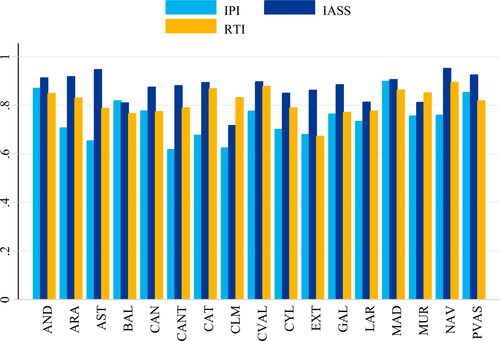
Next, we study the connection that the different productive sectors might have with the aggregate economic activity across the Spanish regions. To this end, we compute the correlation coefficient of several disaggregate measures of the economic activity related to the main economic sectors, with regional GDP growth. To be precise, we compare the correlation coefficient of the IPI, Retail Trade Index (RTI) and Services Sector Activity Index (IASS) with GDPs for all the administrative Spanish divisions (Figure 1). We find clear disparities in the relationship among each disaggregated indicator with GDPs, that provide evidence on the degree of structural heterogeneity across Spanish regions. This result stresses the need for identifying the appropriate set of variables that ought to be used to summarize the evolution of regional GDP in each administrative division.

Figure 1. Correlation with regional GDP growth.

Source: authors own calculations and estimations.

Once we have measured heterogeneity in terms of economic structure and growth across the Spanish regions, we focus on the asymmetric effects of the pandemic. It is important to note that the previous results in this section were computed using the official regional data published by the INE and, as previously mentioned, regional GDP is available at an annual frequency and the last release of this aggregate indicator corresponds to 2019. Therefore, we find evidence of structural heterogeneity before the COVID-19 crisis. Now, given these disparities among the Spanish administrative divisions, we expect the economic effects of a nationwide shock to be asymmetric. In what follows, we review the economic consequences resulting from the implementation of policies aimed at stopping the spread of the virus.

On the 14th of March 2020, the Spanish government announced a state of emergency which affected all the administrative divisions. The state of emergency in Spain imposed severe restrictions in people’s mobility forcing Spanish citizens to stay at home, except for a few activities such as purchasing essential goods or for medical reasons. This measure drastically reduced economic activity. As consequence of the restrictions, Spain showed a sharp and heterogeneous downward evolution across economic sectors during the first and second quarters of 2020. The services sector was the most affected by the virus containment measures and decreased to a larger extent than the industry sector (Banco de España, 2020). Additionally, companies were forced to make use of teleworking when possible. The percentage of people employed who worked online increased from 4.8% to 34% (Peiró & Soler, 2020). However, differences across regions in their capacity to adopt teleworking due to heterogeneous economic structures may also explain the asymmetric consequences of the lockdown.⁸

Thus, it is reasonable to consider that the economic consequences of the lockdown vary over the Spanish regions due to regional heterogeneity. Bearing this in mind, we compare the drop in two key activity indicators, Social Security Contributors (SSC) and IPI, across the 17 Spanish administrative divisions (Figure 2). For SSC indicator, we compute the number of contributors at the end of the month between March to June of 2020 and compute its variation with respect to the same months of the previous year.

Figure 2. Evolution of IPI & SSC during the lockdown.

Source: authors own calculations and estimations.

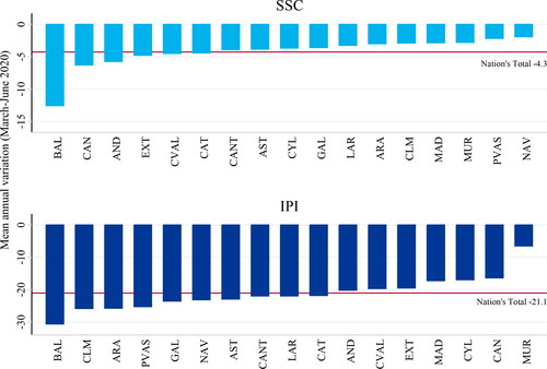
The national decrease in this variable is of 4.3% (red line). Regions as AND, BAL, CAN, CAT, CVAL and EXT show a decrease in the mean annual variation more severe than the national average, while regions as NAV and PVAS experienced a less pronounced drop of about 2%.⁹ The national industrial production, measured with respect to the previous year, shrunk more than 20%. Nonetheless, we find remarkable disparities among the administrative divisions with drops that range between 30.6% in BAL to 6.5% in MUR.

The previous results illustrate differences of economic sectors in regional economic developments and emphasize the need to consider these facts when estimating a indicators of aggregate economic conditions in different regions. This issue will be addressed in Section 4.

3. The model

The methodology followed in order to estimate the common latent factors, capturing the regional aggregate economic developments, has been conditioned by the fact that there is scarcity of macroeconomic regional series. We discuss the regional data availability in the next section.

In particular, we rely on the maximum likelihood estimation of a DFM via the Kalman filter to relate the evolution of a vector of N observed time series, with a latent (or unobserved) common factor, which evolves over time, plus an idiosyncratic part for each individual series.¹⁰

The estimation of the factors via the Kalman Filter allows us to deal with missing values at the end of the panel due to differences in the publication lag of each series and missing values in between the panel for series with different frequencies. This is crucial for our purpose since we can include all the available information in the estimation process with no need to disregard any series in a context strongly conditioned by the shortage of regional macroeconomic indicators.

In this way, we estimate the monthly growth rate of the factor such as the latent force driving a set of variables that enter into the model in annual (x_t) and quarterly (z_t) rates of growth. The variables in annual rates of growth can have either an annual, or a monthly frequency and are modelled as dependent on the last twelve monthly values of the factor (${\sum }_{j=0}^{11}{f}_{t-j}$). Moreover, variables in quarterly rate of growth are related to the factor according to by Mariano and Murasawa (2003). Thus, the set of equations that relate the observable series and the latent factor is: $z_t=\frac{1}{3}{f}_t+\frac{2}{3}{f}_{t-1}+f_{t-2}+\frac{2}{3}{f}_{t-3}+\frac{1}{3}{f}_{t-4}.$ (1) $$\left(\begin{array}{c}{x}_t^1\\ .\\ .\\ .\\ x_t^{n_x}\\ z_t^1\\ .\\ .\\ .\\ z_t^{n_z}\end{array}\right)=\left(\begin{array}{c}{\beta }_1^x{\sum }_{j=0}^{11}{f}_{t-j}\\ .\\ .\\ .\\ {\beta }_{n_x}^x{\sum }_{j=0}^{11}{f}_{t-j}\\ {\beta }_1^z(\frac{1}{3}{f}_t+\frac{2}{3}{f}_{t-1}+f_{t-2}+\frac{2}{3}{f}_{t-3}+\frac{1}{3}{f}_{t-4})\\ .\\ .\\ .\\ {\beta }_{n_z}^z(\frac{1}{3}{f}_t+\frac{2}{3}{f}_{t-1}+f_{t-2}+\frac{2}{3}{f}_{t-3}+\frac{1}{3}{f}_{t-4})\end{array}\right)+\left(\begin{array}{c}{\eta }_t^1\\ .\\ .\\ .\\ {\eta }_t^{n_x}\\ U_t^1\\ .\\ .\\ .\\ U_t^{n_z}\end{array}\right)\mathrm{ }$$(1) where $U_t^i=\frac{1}{3}{u}_t^i+\frac{2}{3}{u}_{t-1}^i+u_{t-2}^i+\frac{2}{3}{u}_{t-3}^i+\frac{1}{3}{u}_{t-4}^i$ for $i=1\dots n^z.$

The dynamics of the latent factor and the idiosyncratic components are also specifically characterized (a = 6, c = 2, b = 6): (2) $$f_t{=\oint }_1^f{f}_{t-1}+\dots +{\oint }_a^f{f}_{t-a}+{ϵ}_t^f$$(2) (3) $${\eta }_t^1={\oint }_1^{{\eta }^1}{\eta }_{t-1}^1+\dots +{\oint }_c^{{\eta }^1}{\eta }_{t-c}^1+{ϵ}_t^{{\eta }^1}$$(3) $$\dots$$ (4) $${\eta }_t^{n_x}={\oint }_1^{{\eta }^{n_x}}{\eta }_{t-1}^{n_x}+\dots +{\oint }_c^{{\eta }^{n_x}}{\eta }_{t-c}^{n_x}+{ϵ}_t^{{\eta }^{n_x}}$$(4) (5) $$u_t^1={\oint }_1^{u^1}{u}_{t-1}^1+\dots +{\oint }_b^{u^1}{u}_{t-b}^1+{ϵ}_t^{u^1}$$(5) $$\dots$$ (6) $$u_t^{n_z}={\oint }_1^{u^{n_z}}{u}_{t-1}^{n_z}+\dots +{\oint }_b^{u^{n_z}}{u}_{t-b}^{n_z}+{ϵ}_t^{u^{n_z}}$$(6)

Finally, ${ϵ}_t^f, {ϵ}_t^{{\eta }^1},{ϵ}_t^{{\eta }^{n_x}},{ϵ}_t^{u^1},$and ${ϵ}_t^{u^{n_z}}$are assumed to be i.i.d. with a normal distribution and zero mean and covariances.

Equations (2)(2) $$f_t{=\oint }_1^f{f}_{t-1}+\dots +{\oint }_a^f{f}_{t-a}+{ϵ}_t^f$$(2) to (6)(6) $$u_t^{n_z}={\oint }_1^{u^{n_z}}{u}_{t-1}^{n_z}+\dots +{\oint }_b^{u^{n_z}}{u}_{t-b}^{n_z}+{ϵ}_t^{u^{n_z}}$$(6) can be included in the following state space representation, using matrices Λ and A: (7) $$Y_t=\Lambda \mathrm{ }{S}_t$$(7) (8) $$S_t=A{S}_{t-1}+vt$$(8) where $Y_t$ is a vector containing the observed $x_t^1,\mathrm{ }\dots x_t^{n_x},\mathrm{ }{z}_t^1,\mathrm{ }\dots z_t^{n_z}$ data at period t and $S_t$ is the state vector equal to ${(f}_t,\mathrm{ }{f}_{t-1},\mathrm{ }\dots ,\mathrm{ }{f}_{t-11},\mathrm{ }{\eta }_t^1,\mathrm{ }{\eta }_{t-1}^1,\mathrm{ }\dots ,{\eta }_t^{n_x},\mathrm{ }{\eta }_{t-1}^{n_x},\mathrm{ }{u}_t^1,\dots ,\mathrm{ }{u}_{t-5\mathrm{ }}^1,\dots ,\mathrm{ }{u}_t^{n_z},\mathrm{ }\dots \mathrm{ }{u}_{t-5}^{n_z})\mathrm{ }$

This representation of the model provides estimates of the factor and parameters in Equation (1)(1) $$\left(\begin{array}{c}{x}_t^1\\ .\\ .\\ .\\ x_t^{n_x}\\ z_t^1\\ .\\ .\\ .\\ z_t^{n_z}\end{array}\right)=\left(\begin{array}{c}{\beta }_1^x{\sum }_{j=0}^{11}{f}_{t-j}\\ .\\ .\\ .\\ {\beta }_{n_x}^x{\sum }_{j=0}^{11}{f}_{t-j}\\ {\beta }_1^z(\frac{1}{3}{f}_t+\frac{2}{3}{f}_{t-1}+f_{t-2}+\frac{2}{3}{f}_{t-3}+\frac{1}{3}{f}_{t-4})\\ .\\ .\\ .\\ {\beta }_{n_z}^z(\frac{1}{3}{f}_t+\frac{2}{3}{f}_{t-1}+f_{t-2}+\frac{2}{3}{f}_{t-3}+\frac{1}{3}{f}_{t-4})\end{array}\right)+\left(\begin{array}{c}{\eta }_t^1\\ .\\ .\\ .\\ {\eta }_t^{n_x}\\ U_t^1\\ .\\ .\\ .\\ U_t^{n_z}\end{array}\right)\mathrm{ }$$(1) by means of the Kalman filter. In addition, when applying the filter, the Kalman gain matrix is modified to give no weight to missing observations in the update equation (see Camacho and Pérez-Quirós (2010) for further details). This modification has the following advantages. It allows us to include the latest available information when estimating the model independently of the publication lag of each series with no need to disregard any information as would imply the use of a balanced panel. It also makes it possible to include series available at different frequencies that are only observed some months within each year. Finally, it is possible to substitute outliers by missing values that will be estimated thanks to their relationship with the other series entering in the model and, therefore, avoiding the replacement of that observation by a certain value decided by the researcher.¹¹

4. Data  availability  and variable selection

In this section, we identify the set of indicators that best captures the aggregate economic evolution in each region. To this end, we investigate the availability of data for the Spanish regions, listing the statistical sources used in previous research for Spain (Artola et al., 2018; Camacho & Doménech, 2012; Camacho & Quiros, 2011; Cuevas et al., 2015). As a result, we find the following official sources of regional macroeconomic data: National Institute of Statistics, Social Security System, National Department of Traffic, Ministry of Industry, Trade and Tourism, CORES,¹² and Eurostat. From these sources, we collect the available series spanning a reasonably long period of time (at least since 2008), prioritizing variables in real terms and those most representative within groups with several indicators measuring disaggregated information about the same macroeconomic concept. The final pool of variables collected after this process includes IPI, RTI, Social Security Contributors (SSC), Employment Regulation Layoffs (ERE), Exports (X), Imports (M), Petrol Consumption (PC), IASS and Overnight Stays¹³ all available at a monthly frequency; Total Labour Cost (TLC) available at a quarterly frequency; and Regional GDP (RGDP) and Income of Households (I) available at an annual frequency. The series were downloaded on September 2020 and span the period from January 2003 to August 2020.

Next, we evaluate which of these series are adequate to capture aggregate regional economic developments. At the national level, Stock and Watson (1991) show that a DFM based on four variables provides estimates of a latent factor which is highly correlated with the Index of Coincident Economic Indicator published by the Department of Commerce in the US. Furthermore, Camacho and Quiros (2011) find that enlarging a set of variables similar to those in Stock and Watson (1991) leads to improved estimates of the factor for monitoring the economic activity in Spain. However, it is important to note that the direct inclusion of more indicators does not necessarily lead to an improvement in estimations. This happens because some series may present cross-correlated idiosyncratic parts and the addition of these series may deteriorate the properties of the estimated factors (Boivin & Ng, 2006). In fact, as acknowledged by Camacho and Pérez-Quirós (2010) highly correlated series may bias the estimation of the factor towards groups of related variables. Thus, we evaluate the consequences of the inclusion of more series and their informational content as follows. Given that the only observable measure of regional aggregate activity that is available is regional GDP, we use this variable as a reference to evaluate the performance of the model and add it to the initial set of variables proposed by Camacho and Pérez-Quirós (2011) for the estimation of a national DFM in Spain (IPI, RTI and SSC). Firstly, for each region, we estimate the model with these four variables (S = 4), which we call the baseline model. Then, we enlarge the initial set of indicators including, one by one, the remaining available variables listed above (S = 5) and compute the percentage of the variance of GDP explained by the estimated factor once the model is enlarged with each candidate series. Then, for each region, we select the series that provides the maximum increase in the GDP’s explained variance to be definitely included into the model. In the following step, the remaining variables are evaluated to include in the model the one that gives the maximum increase of the variance of GDP explained by the new estimated factor with S = 6. This process ends when either we find no more variables able to increase the explained variance of GDP, or when the last available variable is included (S_max=12). We call the resulting model after this process the extended model.

This iterative process provides region-specific datasets to correctly estimate factors that maximize the explained percentage of the variance of the observable measure of aggregate regional economic developments, GDP. In addition, we only include in the model the variables with the highest informational content in order to avoid the inclusion of variables that, if combined, might overrepresent certain macroeconomic concept giving more weight for the estimation of the factors towards it and, consequently, reducing the ability of the factor to explain regional GDP. Finally, we are also able to control for the heterogeneity across regions, providing specific datasets to correctly capture their aggregate economic dynamics. The next section describes the resulting datasets selected in this way for the 17 regions.

5. Results

Variables presented in the Table 2 are obtained using the iterative selection process described in the previous section. Column (1) of the table lists the percentage of the variance of GDP explained by the factor estimated with the baseline model. On average, the initial model explains around 69.5% of the GDP’s variance for the 17 regions and it ranges from 56.68% in EXT to 84.33% in PVAS. Following the table, when the variable listed in the headline (columns (2) to (9)) increases the explained variance of GDP for a region it is included in its extended model and appears as an entry in the corresponding column. Thus, each numerical entry measures the increase in percentage points (pp) in the GDP’s explained variance due to the inclusion of that variable. Empty cells or the cells without a numerical entry point to variables that, once included, lead to estimated factors with less explanatory power of the variance of GDP and which, therefore, were not selected for the extended model. For example, the baseline model of ARA, CYL, CAT, CVAL & LAR is enlarged by one additional variable, while it is enlarged by three more variables in case of AST, BAL, CAN and CANT. We find variables that are included in the extended model and selected for several regions like Income, which is included in thirteen regions, Overnight Stays and the Services Sector Activity Index included in five regions, followed by Imports, which is included in four regions. In addition, we assess the average pp contribution of each variable to the GDP variance explained by the factor. Services Sector Activity Index is the one that has the highest average contribution, 7.17 pp, followed by Overnight Stays with 6 pp and Imports with 5.55 pp. Column (10) reports the percentage of the variance of GDP explained by the factor in the extended model. From this column we can see that the extended model improves the percentage in every region. On average, the extended model explains around 76.5% of GDP variance for the 17 regions. More specifically, AST, BAL, CAN and CLM are the regions that most benefit from the inclusion of additional variables, while ARA, CANT, CAT, and GAL are the regions that benefit the least.

Table 2. Percentage of the variance explained by the common factor by region.

	(1)	(2)	(3)	(4)	(5)	(6)	(7)	(8)	(9)	(10)
		Percentage points increase
Region	Baseline	Total Labor Cost	Income	Overnight Stays	Layoffs	X	M	Petrol consumption	Services Sector Activity Index	Extended model
AND	63.96		1.77						1.61	67.34
ARA	71.01		0.12							71.13
AST	69.46		0.07				20.96		0.38	90.88
BAL	69.06		6.04	0.04					16.12	91.26
CAN	61.88		3.38	29.87			0.95			96.08
CANT	71.02		0.07	0.05			0.02			71.17
CYL	79.41		2.02							81.43
CLM	72.04		1.75						17.45	91.24
CAT	78.22				0.01					78.23
CVAL	57.79	6.04								63.82
EXT	56.68		1.58				0.25			58.52
GAL	77.26		0.18	0.03						77.47
MAD	75.64		1.60	0.01						77.25
MUR	56.82		0.70						0.26	57.78
NAV	74.78	0.48	0.37							75.63
PVAS	84.33	0.12				1.53				85.98
LAR	62.41					1.67				64.08
Average	69.52	2.21	1.51	6.00	0.01	1.60	5.55		7.17	76.43

Source: authors own calculations and estimations.

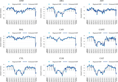
Once we have identified the most informative set of variables for each region, the resulting estimated latent factor captures the heterogeneity in the aggregate activity in each region. The dynamics of the estimated factors are very similar to both national and regional GDPs capturing periods of positive and negative growth. Moreover, we also estimate the unobserved monthly evolution of regional GDP growth based on the factors extracted from each of the regional datasets (Figure 3). To be precise, we relate the monthly factor with annual regional GDP as described in Equation (1)(1) $$\left(\begin{array}{c}{x}_t^1\\ .\\ .\\ .\\ x_t^{n_x}\\ z_t^1\\ .\\ .\\ .\\ z_t^{n_z}\end{array}\right)=\left(\begin{array}{c}{\beta }_1^x{\sum }_{j=0}^{11}{f}_{t-j}\\ .\\ .\\ .\\ {\beta }_{n_x}^x{\sum }_{j=0}^{11}{f}_{t-j}\\ {\beta }_1^z(\frac{1}{3}{f}_t+\frac{2}{3}{f}_{t-1}+f_{t-2}+\frac{2}{3}{f}_{t-3}+\frac{1}{3}{f}_{t-4})\\ .\\ .\\ .\\ {\beta }_{n_z}^z(\frac{1}{3}{f}_t+\frac{2}{3}{f}_{t-1}+f_{t-2}+\frac{2}{3}{f}_{t-3}+\frac{1}{3}{f}_{t-4})\end{array}\right)+\left(\begin{array}{c}{\eta }_t^1\\ .\\ .\\ .\\ {\eta }_t^{n_x}\\ U_t^1\\ .\\ .\\ .\\ U_t^{n_z}\end{array}\right)\mathrm{ }$$(1) . This provides us with the estimates of the annual growth rate of GDP for each month t.

Figure 3. Estimated GDP by region.

Source: authors own calculations and estimations.

The analysed period includes complete business cycles with expansions and contractions covering very volatile periods as the Great Recession and the first stage of the pandemic. We evaluate the accuracy of the extended model at tracking aggregate economic activity along different subsamples. More precisely, we compute the root mean of the squared errors of the model for GDP (RMSE) for the whole sample and compare them with the RMSE corresponding to periods of expansions and contractions as dated by the Spanish Business Cycle Dating Committee. Table 3 shows the ratio of the RMSE for a given period over the RMSE for the whole sample, where entries smaller than one indicate a subperiod where the model performs more accurately than the average. These results show that the extended model captures regional aggregate dynamics with high accuracy during the first stages of the pandemic across all regions.

Table 3. Ratio of GDP Root Mean Squared Error (by subperiod & region) $\frac{\mathit{GDP}\mathit{RMS}{E}_i}{\mathit{GDP}\mathit{RMS}{E}_{\mathit{all}}}$.

i denotes the corresponding row subperiod while all includes all the indicated subperiods. Subperiod dating is done acording to expansions/recessions dated by the Spanish Business Cycle Dating Committee.

	AND	ARA	AST	BAL	CAN	CANT	CYL	CLM	CAT	CVAL	EXT	GAL	MAD	MUR	NAV	PVAS	LAR
2004Q3-2008Q1	0.621	0.556	0.882	0.941	0.928	0.490	0.468	0.761	1.032	0.808	0.232	0.329	0.999	0.837	0.579	0.459	0.944
2008Q2-2009Q4	1.127	2.199	1.330	1.609	1.459	2.167	2.197	2.171	1.681	2.236	2.488	2.339	1.587	1.853	2.621	2.229	1.917
2010Q1-2010Q3	1.851	0.962	1.581	1.336	0.929	0.794	0.886	0.775	1.013	0.956	1.017	0.514	1.004	1.237	0.608	0.791	1.376
2010Q4-2013Q2	1.146	1.248	0.933	0.564	1.215	0.609	0.462	0.329	0.685	0.804	0.605	0.637	0.514	0.447	0.742	0.695	0.271
2013Q3-2019Q3	0.989	0.470	0.941	0.971	0.833	0.928	0.942	0.879	0.888	0.611	0.690	0.861	1.005	0.950	0.372	0.827	0.858
2019Q4-2020Q2	0.202	0.145	0.496	0.232	0.041	0.037	0.038	0.035	0.294	0.139	0.528	0.313	0.256	0.192	0.301	0.766	0.090

Source: authors own calculations and estimations.

Next, we make use of these estimates to track the evolution of regional aggregate activity month by month. In particular, we pay attention to economic developments during the first stage of the pandemic.

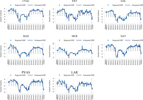
Figure 3. Estimated GDP by region - panel B.

Figure 4 presents the estimations of the evolution of GDP for all the regions from January to August 2020 covering the lockdown and its aftermath. The vertical lavender dashed-line indicates the beginning of the lockdown (March 2020) in Spain. As expected, we find a general decrease in the evolution of the estimated GDP during these months in every region. However, our results show some differences in the magnitude of this fall and the subsequent recovery across regions.

Figure 4. Estimated GDP by region.

Source: authors own calculations and estimations.

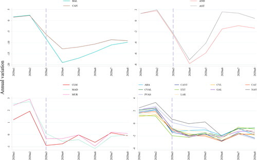
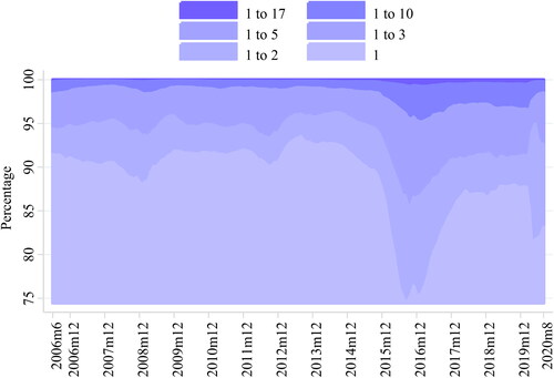
Figure 5. Percentage of the variance explained by different number of eigenvalues.

Source: authors own calculations and estimations.

We classify regions according to the size of the drop in their estimated GDP after the lockdown as follows: BAL and CAN show the sharpest decline in economic activity, −19% and −12.8% respectively, and are still far from reaching positive rates of growth during July and August. These two cases might be explained by the weight that tourism has in the two regions.¹⁴ In fact, in the selection variable process for these regions, we find that Overnight Stays, an indicator that strongly mirrors touristic activity, is a variable with useful informational content to explain aggregate economic activity in our extended model. AND and AST also show a drastic decrease in economic activity of −7.78% and −7.12%, respectively. However, they show a trend change, reaching positive growth rates from April to June.

CLM, MAD and MUR show a smaller decrease during the lockdown and even reach positive or close to positive growth rates during the last months of the sample. Interestingly, in most of these regions the Services Sector Activity Index was selected as an indicator that improves the factor in explaining GDP throughout the sample. Thus, a smaller or shorter economic downturn in these regions could be explained if teleworking has been a common practice in the activities belonging to the service sector.

ARA, CANT, CYL, CAT, CVAL, EXT, GAL, NAV, PVAS and LAR show an intermediate reduction of economic activity ranging from −1.88% to −2.84%. However, none of these regions show a clear recovery since the lockdown up to the end of the sample period.

At this point, once we have measured the regional economic impact of the pandemic, we evaluate the consequences of a shock, affecting the Spanish territories simultaneously but unevenly, on the macroeconomic co-movements among the Spanish regions. To this end, we assess the evolution of the overall degree of inter-connectedness or synchronization in growth among the 17 Spanish administrative divisions as in Billio et al. (2012). These authors measure the connectedness among several financial institutions through the eigenvalue analysis of their returns. To be precise, Billio et al. (2012) associate periods of high inter-connectedness among institutions with moments when a few eigenvalues of the data matrix are able to explain a larger percentage of its total variation. Thus, we apply the eigenvalue decomposition to the 17 estimated monthly GDPs using a 36-month rolling-window sample period. This approach is particularly appealing since it allows us to obtain a dynamic measure that summarizes the degree of synchronization for the whole set of Spanish regions, instead of evaluating it pairwise.

Figure 5 depicts the evolution of the percentage of the data variance explained by the group of 17 eigenvalues. As previously mentioned, the higher this percentage is, the stronger the co-movements among the regional economic developments for the whole country are. The biggest eigenvalues are able to explain a high proportion of the variability in the data reflecting significant inter-connectedness among the Spanish regions. However, the relevance of the first eigenvalues explaining these economic co-movements varies substantially over time. After 2013–2014, the Spanish administrative divisions started a period of positive growth. Nonetheless, not all the regions grew at the same pace as it is reflected by the annual official data published by INE (Figure 3). The decrease in the explanatory power of the first eigenvalues captures this decoupling in the economic developments across the Spanish regions during this period of unequal economic performance. After 2017, the regions show a process of convergence towards similar growth rates to those shown in 2018 and 2019, around 2% according to the official data. The increase in the synchronicity was suddenly accelerated during March 2020 when the explained variance by the eigenvalues shows a sharp increase. This coincides with the lockdown and the restrictions to prevent the spread of the virus, when economic activity abruptly stopped nationwide.

6. Conclusions

The COVID-19 crisis has brought renewed attention towards the analysis of regional economic developments. The policies to stop the spread of the virus are implemented rapidly and their economic consequences require measuring economic activity with high frequency. The economic effects of these measures vary across regions due to the diversity in their economic structures and the different pace in the removal of the restrictions after the first stages of the pandemic in each region. However, the available regional aggregate indicators for the evaluation of these policies, such as GDP, are released at a low frequency and published with considerable delay. More importantly, even though official bodies provide a number of disaggregate macroeconomic regional indicators, they are scarce and only contain partial information of the regional economic activity. Furthermore, Spanish administrative divisions show heterogeneous economic structures that require the identification of the most relevant available indicators to evaluate the economic situation in each region. Therefore, we provide estimates of the regional aggregate economic activity at a monthly frequency conditional on the data availability and structural heterogeneity of the 17 Spanish administrative divisions. To this end, we combine a Dynamic Factor Model, that allows us to summarize a set of variables regardless of their frequency and publication lag into a latent monthly factor, with an iterative process that identifies the set of variables that maximizes the power of the factor to explain regional GDP.

Our results support the presence of heterogeneity in the economic structures of the Spanish regions. The region-specific sets of indicators resulting from the variable selection process show that the series with the highest informational content to explain regional GDPs vary substantially across regions. Some variables are relevant for a large group of regions, as Income, while other indicators, as the Services Sector Activity Index, are only selected for a few regions. These findings, about the differences in the most adequate set of indicators, set the ground for the future evaluation of new potential indicators, which may become available and improve the performance of the extended model, primarily for regions where the extended model explains smaller percentages of regional GDPs.

In addition, we use these aggregate regional indicators to measure the economic developments over the Spanish regions during the first stage of the pandemic using monthly estimates of regional GDP. As result, we identify remarkable asymmetries in the economic effects of the COVID-19 shock. We find regions with a productive structure that is highly oriented towards the tourism industry that show a more severe economic downturn, while there are regions with a highly notable services sector that tend to recover faster. Our results show that the models, including data for the first stage of the pandemic, can capture the economic dynamics of this initial stage with high precision. Nonetheless, the performance of the models should be reevaluated in future research once the recovery concludes and data corresponding to a more stable environment become available.

Moreover, we take further advantage of the monthly estimates of aggregate regional activity to evaluate the evolution of economic synchronization among the Spanish administrative divisions. The results show that Spanish regions experienced a decoupling in their economic performance during the recovery period that followed the European sovereign debt crisis, when some regions were able to achieve faster economic growth. It is important to note that during this period the Spanish regions were not able to comply with fiscal discipline. As Delgado-Téllez et al. (2017) point out, errors in the forecast of annual GDP have a statistically significant effect on regional fiscal non-compliance in the aftermath of the sovereign debt crisis. The availability of high frequency accurate estimates of the regional economic developments in that period would have been useful to optimize fiscal targets and facilitate the recovery across regions.

We find, the same pattern of discrepancies in regional recovery after the first stage of the pandemic. Thus, policymakers must devote particular attention to regional developments and to evaluate the effects of the pandemic conditional on regional economic heterogeneity.

We restricted our analysis to the lockdown period of the pandemic when measures for the containment of the virus were applied nationwide and equally to all regions. This allowed us to isolate the asymmetric effects of homogeneous policies applied nationwide. However, it is important to note that, once the state of emergency ended in Spain, each region was given the power and responsibility to monitor the evolution of the pandemic and to adopt the necessary containment measures. Furthermore, most of the EU funds aim to promote the economic recovery received by the central government in Spain will be distributed among the Spanish regional governments. Thus, it is reasonable to consider that under the implementation of different regional policies to stop the spread of the virus and to promote economic recovery, combined with differences the regional institutional quality, the Spanish subnational divisions will show differences in their paces of recovery. In this situation, our estimates facilitate the early monitoring of the effects of such policies and assist decisions on the timing to remove these stimuli and, importantly, in which regions.

To conclude, the results presented here provide new insights into the specific economic characteristics of each Spanish administrative division. Additionally, they emphasize that policymakers must closely monitor regional economic fluctuations in order to improve their decision-making process, not only due to the pandemic, but also because of the expected increase in regional heterogeneity predicted by the OECD (2021) and to evaluate the efficiency of the policies granted by the NextGeneration EU funds. As a result, it is necessary a greater effort from public institutions and official statistics offices to provide richer regional economic information at a higher periodicity.

Disclosure statement

No potential conflict of interest was reported by the authors.

Additional information

Funding

This work was supported by the Catholic University of Murcia under Grant (PMAFI-COVID19/06).

Notes

1 The rolling 7-day average of the daily new confirmed COVID-19 cases per million people on 13th of March was 14.76 in Spain and 9.04 in EU and two weeks after 46.38 and 26.25, respectively (Ritchie el al., 2020).

2 Quarterly updated estimates of Koop et al. (2020) are available online: ttps://www.escoe.ac.uk/regionalnowcasting/

3 See Leiva-León et al. (2020) and Lewis et al. (2020) for the estimation of high frequency latent indicators at the global and national level, respectively.

4 In their approach, Bakarić et al. (2016) obtain a first characterization of the business cycle applying a Markov Switching to the Croatian GDP for the selection of the variables. We do not follow this approach here since GDP series for the Spanish regions are available at an annual frequency and span a short period.

5 In a previous paper, Gadea et al. (2012) show that regional business cycles within Spain are quite heterogeneous.

6 We label the 17 Spanish Autonomous Communities according to the NUTS-2 EUROSTAT’s nomenclature. The regions are: Andalucía (AND), Aragón (ARA), Asturias (AST), Baleares (BAL), Canarias (CAN), Cantabria (CANT), Castilla y León (CYL), Castilla-La Mancha (CLM), Cataluña (CAT), Comunidad Valenciana (CVAL), Extremadura (EXT), Galicia (GAL), Comunidad de Madrid (MAD), Región de Murcia (MUR), Navarra (NAV), País Vasco (PVAS) and La Rioja (LAR).

7 In their paper, Díaz-Lanchas and Mulder (2021) analyse the role that government decentralization plays on the diversification of the local productive structures and find that an increase in institutional quality over time increases the probability of diversification. In a similar vein, Guillamón and Cuadrado-Ballesteros (2021) analyse the determinants of the variation in the efficiency of Spanish local governments during 2008 and 2014 and find that more transparent administrations tend to be more efficient in the provision of public services.

8 Aspects like the economic sector, type of occupation, type of employment contract, the technological equipment and the workers’ socio-demographic characteristics determine the teleworking capacity across Spain (Anghel et al., 2020).

9 This result is in accordance with Almeida et al. (2020) who previously found that unemployment in the Mediterranean regions is more sensitive to the economic conditions.

10 In this estimation method it is assumed that the idiosyncratic part of the series entering in the model presents no cross-correlation (exact DFM). Camacho and Pérez-Quirós (2010) and Stock and Watson (1991) have shown that this estimation procedure has a good performance despite this assumption.

11 In our application we cover a period including the Great Recession as well as the lockdown during the first wave of the pandemic so, it is possible to find some outliers in the series. In this regard, we follow Stock and Watson (2002) and consider outliers those values of the series that exceed 10 times the interquartile range, which we replace by a missing value. McCracken and Ng (2020) follow the same approach and find that, even though the removal of these observation is debatable, the replacement of the outliers by missing values has minimal effects on the estimated factors.

12 Corporación de Reservas Estratégicas de Productos Petrolíferos

13 Number of nights spent by foreigners in Spanish hotels.

14 BAL and CAN are two groups of islands in the Mediterranean Sea and the Atlantic Ocean, respectively. In these regions, the tourism industry is very important as it provides jobs to a large proportion of the population.

References

- Almeida, A., Galiano, A., Golpe, A. A., & Martín, J. M. (2020). Regional unemployment and cyclical sensitivity in Spain. Letters in Spatial and Resource Sciences, 13(2), 187–199. https://doi.org/10.1007/s12076-020-00252-3
- Alvaréz, R., Camacho, M., & Perez-Quiros, G. (2016). Aggregate versus disaggregate information in dynamic factor models. International Journal of Forecasting, 32(3), 680–694. https://doi.org/10.1016/j.ijforecast.2015.10.006
- Anghel, B., Cozzolino, M., & Lacuesta Gabarain, A. (2020). El teletrabajo en España. Boletín Económico/Banco de España [Artículos], n. 2, 2020, 1–18.
- Artola, C., Gil, M., Pérez, J. J., Urtasun, A., Fiorito, A., & Vila, D. (2018). Monitoring the Spanish economy from a regional perspective: Main elements of analysis. (No. 1809). Banco de España.
- Billio, M., Getmansky, M., Lo, A. W., & Pelizzon, L. (2012). Econometric measures of connectedness and systemic risk in the finance and insurance sectors. Journal of Financial Economics, 104(3), 535–559. https://doi.org/10.1016/j.jfineco.2011.12.010
- Blanchard, O., Philippon, T., & Pisani-Ferry, J. (2020). A new policy toolkit is needed as countries exit COVID-19 lockdowns (pp. 20–28). Bruegel.
- Boivin, J., & Ng, S. (2006). Are more data always better for factor analysis? Journal of Econometrics, 132(1), 169–194. https://doi.org/10.1016/j.jeconom.2005.01.027
- Camacho, M., & Doménech, R. (2012). MICA-BBVA: A factor model of economic and financial indicators for short-term GDP forecasting. SERIEs, 3(4), 475–497. https://doi.org/10.1007/s13209-011-0078-z
- Camacho, M., & Pérez-Quirós, G. (2010). Introducing the euro‐sting: Short‐term indicator of euro area growth. Journal of Applied Econometrics, 25(4), 663–694. https://doi.org/10.1002/jae.1174
- Camacho, M., & Quiros, G. P. (2011). Spain‐sting: Spain short‐term indicator of growth. The Manchester School, 79, 594–616. https://doi.org/10.1111/j.1467-9957.2010.02212.x
- Crone, T. M., & Clayton-Matthews, A. (2005). Consistent economic indexes for the 50 states. Review of Economics and Statistics, 87(4), 593–603. https://doi.org/10.1162/003465305775098242
- Cuevas, A., Quilis, E. M., & Espasa, A. (2015). Quarterly regional GDP flash estimates by means of benchmarking and chain linking. Journal of Official Statistics, 31(4), 627–647. https://doi.org/10.1515/jos-2015-0038
- de España, B. (2018). Informe trimestral de la Economía española (Boletín económico 1/2020).
- Delgado-Téllez, M., Lledo, V. D., & Pérez, J. J. (2017). On the determinants of fiscal non-compliance: An empirical analysis of Spain’s regions. International Monetary Fund.
- Díaz-Lanchas, J., & Mulder, P. (2021). Does decentralization of governance promote urban diversity? Evidence from Spain. Regional Studies, 55(6), 1111–1128. https://doi.org/10.1080/00343404.2020.1863940
- Fedajev, A., Radulescu, M., Babucea, A. G., Mihajlovic, V., Yousaf, Z., & Milićević, R. (2022). Has COVID-19 pandemic crisis changed the EU convergence patterns? Economic Research-Ekonomska Istraživanja, 35(1), 2112–2141. https://doi.org/10.1080/1331677X.2021.1934507.
- Gadea, M. D., Gómez-Loscos, A., & Montañés, A. (2012). Cycles inside cycles: Spanish regional aggregation. SERIEs, 3(4), 423–456. https://doi.org/10.1007/s13209-011-0068-1
- Guillamón, M. D., & Cuadrado-Ballesteros, B. (2021). Is transparency a way to improve efficiency? An assessment of Spanish municipalities. Regional Studies, 55(2), 221–233. https://doi.org/10.1080/00343404.2020.1772964
- Instituto Nacional de Estadística. (2019). Contabilidad Regional de España. Serie 2016–2019. https://www.ine.es/CDINEbase/consultar.do?mes=&operacion=Contabilidad+Regional+de+Espa%F1a&id_oper=Ir&L=0
- Koop, G., McIntyre, S., Mitchell, J., & Poon, A. (2020). Regional output growth in the United Kingdom: More timely and higher frequency estimates from 1970. Journal of Applied Econometrics, 35(2), 176–197. https://doi.org/10.1002/jae.2748
- Lehmann, R., & Wohlrabe, K. (2015). Forecasting GDP at the regional level with many predictors. German Economic Review, 16(2), 226–254. https://doi.org/10.1111/geer.12042
- Leiva-Leon, D., Pérez-Quirós, G., & Rots, E. (2020). Real-time weakness of the global economy: A first assessment of the coronavirus crisis. Working paper series at the European Central Bank, No 2381. https://www.ecb.europa.eu/pub/pdf/scpwps/ecb.wp2381∼444d6f578f.en.pdf
- Lewis, D., Mertens, K., & Stock, J. H. (2020). US economic activity during the early weeks of the SARS-Cov-2 outbreak. (No. w26954). National Bureau of Economic Research.
- Mariano, R. S., & Murasawa, Y. (2003). A new coincident index of business cycles based on monthly and quarterly series. Journal of Applied Econometrics, 18(4), 427–443. https://doi.org/10.1002/jae.695
- McCracken, M., & Ng, S. (2020). FRED-QD: A quarterly database for macroeconomic research. (No. w26872). National Bureau of Economic Research.
- OECD. (2021). OECD Economic Surveys: Spain 2021. OECD Publishing. https://doi.org/10.1787/79e92d88-en
- Peiró, J. M., & Soler, A. (2020). El impulso al teletrabajo durante el COVID-19 y los retos que plantea. IvieLAB, 1, 1–10.
- Prieto, A. D. (2020, April 9). Sánchez anuncia su plan de desescalada: medidas semanales y una app para controlar a la población. El Español. https://www.elespanol.com/espana/politica/20200409/sanchez-anuncia-desescalada-semanales-app-controlar-poblacion/481202209_0.html
- Rašić Bakarić, I., Tkalec, M., & Vizek, M. (2016). Constructing a composite coincident indicator for a post-transition country. Economic Research-Ekonomska Istraživanja, 29(1), 434–445. https://doi.org/10.1080/1331677X.2016.1174388
- Ritchie, H., Mathieu, E., Rodés-Guirao, L., Appel, C., Giattino, C., Ortiz-Ospina, E., Hasell, J., Macdonald, B., Beltekian, D., & Roser, M. (2020). Coronavirus pandemic (COVID-19). In Kajal Lahiri & Geoffrey H. Moore (Eds.), Our world in data (pp. 63–90). Cambridge University Press.
- Stock, J. H., & Watson, M. W. (1991). A probability model of the coincident economic indicators. In K. Lahiri & G. H. Moore (Eds.), Leading economic indicators: New approaches and forecasting records (pp. 147–162). Cambridge University Press.
- Stock, J. H., & Watson, M. W. (2002). Macroeconomic forecasting using diffusion indexes. Journal of Business & Economic Statistics, 20(2), 147–162. https://doi.org/10.1198/073500102317351921