Downside and upside risk spillovers from commercial banks into China’s financial system: a new copula quantile regression-based CoVaR model

Abstract

In this paper, we investigate the downside and upside risk spillovers from three kinds of commercial banks (state-owned commercial banks (SOCBs), joint-stock commercial banks (JSCBs) and city commercial banks (CCBs)) to China’s financial system by proposing a new copula quantile regression-based CoVaR model. We find that (i) the dynamic risk spillovers show heterogeneity over time, specifically that its downward trend is significant after the stock market disaster in 2015; (ii) JSCBs display the largest risk spillovers, indicating that JSCBs are the main contributors to systemic risk in China’s financial system; and (iii) the risk spillovers are not symmetrical, as the upside risk spillovers are smaller than the downside risk spillovers. Our results have crucial implications for financial regulators and investors who want to measure and prevent systemic financial risk and optimise their investment strategies.

Keywords:

• Risk spillover effect
• banking sector
• CoVaR
• copula quantile regression
• bootstrap Kolmogorov-Smirnov test

Subject Classification Codes::

• C51
• C53
• G21

1. Introduction

In this paper, we investigate the dynamic downside and upside risk spillovers from the banking sector to the Chinese financial system by proposing a new copula quantile regression (CQR)-based CoVaR model with a skewed Student’s t (SKST) distribution as the margins of the copula function. Financial intermediates in China are dominated by its banking sector, which plays a vital role in the development of the national economy (Medina-Olivares et al., 2022; Sun et al., 2022; Yang et al., 2019; Ye et al., 2019). According to the China Banking Regulatory Commission (CBRC), the total assets of China’s banking industry, at 268 trillion Yuan, account for 89% of the total assets of China’s financial industry in 2018. Because of its dominant position in the financial system, the banking sector is an important area of risk management for China. Therefore, studying the risk spillovers of the banking sector into the financial system is of considerable significance to China’s risk governance.

China’s banking sector has experienced a tortuous development process since China’s reform and opening up in 1978. Presently, it comprises a three-pronged structure including state-owned commercial banks (SOCBs), joint-stock commercial banks (JSCBs) and city commercial banks (CCBs). Based on the CBRC data, the banking sector had 4,571 banks by the end of 2018. Among them, SOCBs had the largest market share (36.67%), JSCBs had the second largest market share (17.53%) and CCBs had the third largest market share (12.80%). Since the global financial crisis of 2008–2009, to curb the economic downturn and achieve a stable, high-quality economic growth target, the banking sector of China rapidly expanded the total credit under a request from the government (Zhu, 2021). Based on data from the Bank for International Settlements, the debt-to-GDP ratio of non-financial sectors (government, households and corporations) in China increased from 147.5% in 2007 to 254.8% in 2018, with an annual growth rate of 5.1%. International experience has shown that the rapid expansion of credit may lead to financial crises, decelerating economic growth or both (Dell’Ariccia et al., 2016). Therefore, one must consider the increased risk in the banking sector caused by the increasing levels of credit for non-financial sectors in China.

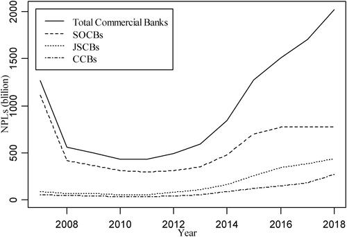
In addition, the increasing non-performing loans (NPLs) held by the Chinese banking sector constitute another problem that China must face. Figure 1 shows the dynamic NPLs held by the three commercial banks and the entire banking sector in China from 2007 to 2018. Overall, the dynamic NPLs held by China’s banking sector shows a U-shaped curve. More specifically, these NPLs declined since the outbreak of the financial crisis, reaching their lowest level around 2011. However, after 2011, NPLs began to grow at a rate of about 10%. We also find that the three kinds of commercial banks held different scales of NPLs, for which the evolution trends are also different. These observations indicate that the risks exposed by these three types of commercial banks may are also heterogeneous. In summary, we find that NPLs and market shares held by different commercial banks are not the same over time. A natural question then is raised: do banks with more NPLs and higher market share contribute more to the system risk? To this end, one purpose of this paper is to measure and rank spillovers from different kinds of commercial banks into the financial system in China.

Figure 1. The dynamics of NPLs in the banking sector (Data source: CBRC).

Our second motivation is to propose a new framework for calculating CoVaR and risk spillover. Presently, the CoVaR model is widely applied to measure risk spillovers due to its efficiency and accuracy. From a statistical perspective, CoVaR is measured using the conditional quantiles of return distributions at a specific significance level. Generally, CoVaR could be estimated by linear quantile regression that has been practiced by many scholars (e.g., Acharya et al., 2012; Adrian & Brunnermeier, 2016; Ameur et al., 2020; Bernal et al., 2014; Lin et al., 2018; Tiwari et al., 2022). However, estimating by linear quantile regression ignores the nonlinearity of tail dependence between financial variables and can lead to biased estimates in computing CoVaR and risk spillovers (López-Espinosa et al., 2015).

To address this issue, this paper develops a new CQR-based CoVaR model combining the nonlinear CQR model with the CoVaR approach. In the pioneering paper by Bouyé and Salmon (2009), they gave the analytical expression of the Clayton CQR model which can capture the lower tail dependence and estimate the spillover effects of the downside risk. Compared with the abundance of research on downside risk spillovers, there are only few studies on upside risk and its spillovers (Ameur et al., 2020; Ji et al., 2020; Reboredo et al., 2016; Warshaw, 2019). However, upside risk is another kind of systemic financial risk because it may result in more severe future losses and higher uncertainty. Therefore, to maintain financial stability, regulators need to simultaneously measure the downside and upside risk spillovers in the financial system to prevent systemic risk and improve macroprudential management. However, Bouyé and Salmon (2009) did not give the analytical expression of the Gumbel CQR model which can describe the upper tail dependence and calculate the upside risk spillovers accurately. In this paper, we use a transcendental function to solve this problem for the first time and give the parameter estimation method of the Gumbel CQR model.

The advantage of our new framework lies in three aspects. First, this approach can capture the nonlinearity of downside and upside tail dependence among financial variables. Second, this approach uses an SKST distribution as the margins of the copula function, which can accurately characterise the properties of sharp peaks, fat tails and skewness in the return distributions. Third, this approach allows us to estimate the dynamic downside and upside risk spillovers using rolling window method.

This study contributes to the existing literature in the following ways. First, we propose a new CQR-based CoVaR model, which integrates the Clayton and Gumbel CQR models into the CoVaR approach. To the best of our knowledge, we are the first to estimate CoVaR based on the Clayton and Gumbel CQR models. Second, we explore the downside and upside risk spillovers from three commercial banks to the overall financial system in China from both static and dynamic perspectives. Our study proves that the risk from the banking sector plays a vital role in the risk accumulation in China’s financial system. Additionally, the dynamic risk spillovers show heterogeneity over time, specifically the downward trend is significant after the stock market disaster in 2015. Third, we assess dominance and asymmetry by conducting a two-sample bootstrap Kolmogorov-Smirnov (KS) test (Abadie, 2002). Based on the results of these tests, we find that JSCBs display the largest upside and downside risk spillovers among these three kinds of banks, indicating that JSCBs contribute the most to China’s financial system. We also find that the risk spillovers are not symmetric, with a smaller upside risk spillover than downside risk spillover that are consistent with the flight-to-quality phenomenon.

The remainder of this paper is organised as follows. Section 2 provides a review of the literature. Section 3 introduces the theoretical framework of the CQR-based CoVaR model. Section 4 describes the data and some preliminary statistics. Sections 5 and 6 discuss the empirical results and policy implications, respectively. Section 7 draws conclusions.

2. Literature review

In this section, we review the literature on systemic risk measures and the impact of banking section risk on system risk. A large amount of research has shown that risk in individual banks is contagious to other banks and even the financial system in the worldwide (see Adams et al., 2014; Bernal et al., 2014; Billio et al., 2012; Borri & Giorgio, 2022; Ghulam & Doering, 2018; Girardi & Ergün, 2013; Pham et al., 2021). For example, Adams et al. (2014) claimed that commercial banks appear to play a major role in the financial market compared to other financial institutions in volatile market periods. Borri and Giorgio (2022) considered 35 European banks and found that all banks significantly contribute to systemic risk, but larger banks, and banks with a business model more exposed to financial markets, contribute more. Moreover, many studies show that the banks with larger assets have greater systemic risk. Laeven et al. (2016) confirmed that systemic risk increases with the growth of bank size, though it is inversely proportional to bank capital. Kolari et al. (2020) argued that large banks play an important role in the volatility in systemic risk. In China, the financial system is dominated by the banking sector, indicating that systemic risk in the banking sector may have considerable impact on the financial system. Xu et al. (2018) argued that banks with larger assets and state-owned nature, were systemically important institutions. Ouyang et al. (2020) used a directed network approach to measure the systemic risk contagion effect of the Chinese banking industry and found that the financial system becomes more closely related and the current bank is characterised by the phrases ‘too big to fail’ and ‘too connected to fail’. However, Fan et al. (2017) showed that the banks with large asset scale had great risk spillovers, but some of the smaller scale banks also had greater risk contribution in the risk period. By using the wavelet-based quantile regression model, Xu et al. (2021) also found that banks with smaller size and higher leverage had more contributions to the systemic risk.

All in all, there is no unanimous conclusion on the identification of systemically important banks (SIBs), so further research is needed. The existing literature provides a good reference for our study. Inspired by them, we put forward our preliminary research hypothesis that (i) the dynamic risk spillovers from the three kinds of banks (SOCBs, JSCBs and CCBs) into the financial system may show heterogeneity at some specific periods; (ii) SOCBs with a larger market share in China’s bank system may not contribute more systemic risk in China’s financial system, as evidenced by Wang et al. (2017, 2018); and (iii) the risk spillovers may are not symmetrical, which means that the upside risk spillovers are not equal to the downside risk spillovers.

Developing new methods to measure systemic risk is necessary since academics and regulators have not reached a consensus on a method that can accurately compute financial risk (Adrian & Brunnermeier, 2016). The most frequently used method for measuring systemic risk is through measuring co-dependence in the tails of equity returns of an individual financial institution and the financial system. Bisias et al. (2012) categorise the current approaches to measuring systemic risk along the following lines: tail measures, contingent claims analysis, network models and dynamic stochastic macroeconomic models.

Some scholars focus primarily on constructing networks in the interbank system (Glasserman & Young, 2015; Raffestin, 2014; Roukny et al., 2018), and secondarily on estimating systemic risk spillovers. The second strand of literature investigates measures of potential risk spillovers, such as CoVaR, the CoES (conditional expected shortfall) (Adrian & Brunnermeier, 2016), the marginal expected shortfall (Acharya et al., 2017), the systemic risk measure (Acharya et al., 2012) and the systemic risk index (Brownlees & Engle, 2017).

The CoVaR model can effectively and simply estimate potential risk spillovers and hence is widely used in risk management (Bernardi et al., 2017; López-Espinosa et al., 2015; Teply & Kvapilikova, 2017). As CoVaR is a conditional quantile, it can be computed via linear quantile regression (Acharya et al., 2012; Adrian & Brunnermeier, 2016; Ameur et al., 2020; Bernal et al., 2014). However, this method ignores the reality that financial variables are nonlinearly correlated at high risk levels. Thus, calculating CoVaR using a linear quantile regression model may result in biased estimates of potential risk spillovers.

As is known, the copula function, which is one of the most useful tools for capturing nonlinear tail dependence between financial variables, has been used to calculate risk spillovers (Ji et al., 2019; Karimalis & Nomikos, 2018; Reboredo et al., 2016; Reboredo & Ugolini, 2015; Warshaw, 2019; Xiao, 2020; Yang et al., 2020). Especially, Bouyé and Salmon (2009) proposed a CQR model which has proved to be accurate in capturing the nonlinearity of downside and upside tail dependence. However, the CQR model has not yet been used for risk spillover analysis. Therefore, we provide a new framework for calculating CoVaR based on the CQR model to verify our hypothesis proposed in this paper.

3. A new CQR-based CoVaR model

In this section, we first introduce the marginal distribution of SKST distribution. Second, we provide the estimation method of the Clayton and Gumbel CQR models with SKST distribution as marginal distribution. Third, we explain in detail how to use the Clayton and Gumbel CQR models to estimate the downside and upside CoVaR. Lastly, under the framework of the CQR-based CoVaR model, we provide the estimates of the static and dynamic risk spillovers.

3.1. Marginal distribution

In the field of risk management, the return distribution of financial variables generally exhibits the properties of both kurtosis and skewness, which does not follow Student’s t distribution. In view of this, we use the SKST distribution to capture the properties of financial variables. Letting $X\sim \mathit{SKST}\left(\mu ,\sigma ,\upsilon ,\gamma \right)$ be the SKST distribution, its probability density function (PDF) is (1) $$f\left(x\right)=\frac{2\Gamma \left(0.5\right(\vartheta +1\left)\right)\mathrm{\sigma }{(1+{\vartheta }^{-1}{\sigma }^2{\left(x-\mu \right)}^2({\gamma }^{-2}{I}_{[0,\mathrm{\infty })}\left(x-\mu \right)+{\gamma }^2{I}_{[0,\mathrm{\infty })}\left(x-\mu \right)\left)\right)}^{-0.5(\vartheta +1)}}{\Gamma \left(\vartheta /2\right){\left(\pi \vartheta \right)}^{0.5}(\gamma +{\gamma }^{-1})}$$(1) where $\mu$ is the location parameter, indicating the expectation of the variable; $\sigma >0$ is the scale parameter, indicating the volatility of the variable; $\vartheta >2$ is the shape parameter, indicating the thickness of the tails; and $\gamma >0$ is the skewness parameter, indicating the allocation of mass to each side of the mode. We can estimate the parameters of the SKST distributions using maximum likelihood estimation (MLE).

3.2. Clayton and Gumbel CQR models

The Archimedean copula is the most widely used in financial risk management (Charpentier & Segers, 2007). An Archimedean copula function is $C\left(u,v\right)={\varphi }^{-1}(\varphi (u)+\varphi (v))$ for different generator functions denoted by $\varphi .$ The conditional probability of $v,$ given $U=u,$ can be obtained by the first partial derivatives of the Archimedean copula function on $u.$ That is, (2) $$P\left(V\le v\right|U=u)=\partial C(u,v)/\partial u.$$(2)

At quantile $\tau \in (0,1),$ solving for $\tau =\partial C(u,v)/\partial u,$ Bouyé and Salmon (2009) obtained the Archimedean CQR curve as follows: (3) $$v={\varphi }^{-1}\left(\varphi \left({\varphi }^{\mathrm{\prime }-1}\left(\frac{{\varphi }^{\mathrm{\prime }}\left(u\right)}{\tau }\right)\right)-\varphi \left(u\right)\right),$$(3) where ${\varphi }^{-1}$ and ${\varphi }^{\prime }$ are the inverse function and derivative function of $\varphi ,$ respectively.

Using a generator function $\varphi (t)$ with $\varphi \left(t\right)=t^{-\delta }-1$ and $\varphi \left(t\right)={(-lnt)}^{\delta },$ we obtain the Clayton and Gumbel copula functions as follows: (4) $$C^C\left(u,v\right)={(u^{-\delta }+v^{-\delta }-1)}^{-1/\delta },\delta >0$$(4) (5) $$C^G\left(u,v\right)=\hspace{0.17em}{\text{exp}({-\left(\right(-\mathit{ln}u)}^{\delta }+{(-\mathit{ln}v)}^{\delta })}^{1/\delta }),\delta \ge 1,$$(5) in which $\delta$ describes the degree of downside (for the Clayton copula) and upside (for the Gumbel copula) tail dependence between the two variables $u$ and $v$ (Nelsen, 2006).

Based on Equation (3)(3) $$v={\varphi }^{-1}\left(\varphi \left({\varphi }^{\mathrm{\prime }-1}\left(\frac{{\varphi }^{\mathrm{\prime }}\left(u\right)}{\tau }\right)\right)-\varphi \left(u\right)\right),$$(3) and the generator function $\varphi \left(t\right)=t^{-\delta }-1,$ the corresponding Clayton CQR curve of $v,$ given $U=u$ at quantile $\tau ,$ is as follows: (6) $$v={\left(\right({\tau }^{-\delta /(1+\delta )}-1)u^{-\delta }+1)}^{-1/\delta }.$$(6)

However, for the Gumbel copula, we can obtain everything in Equation (3)(3) $$v={\varphi }^{-1}\left(\varphi \left({\varphi }^{\mathrm{\prime }-1}\left(\frac{{\varphi }^{\mathrm{\prime }}\left(u\right)}{\tau }\right)\right)-\varphi \left(u\right)\right),$$(3) except ${\varphi }^{\prime -1}.$ Thus, the Gumbel CQR curve cannot be derived analytically. Combining the Gumbel copula function with its generator function $\varphi \left(t\right)={(-lnt)}^{\delta },$ we obtain the following equation for quantile $\tau :$ (7) $$\tau =\partial C^G(u,v)/\partial u=u^{-1}{\left(-\mathit{ln}u\right)}^{\delta -1}{({(-\mathit{ln}u)}^{\delta }+{(-\mathit{ln}v)}^{\delta })}^{(1-\delta )/\delta }{C}^G\left(\mathrm{u},v\right).$$(7)

Then, formula (7) is equivalent to $\tau =u^{-1}{\left(-\mathit{ln}u\right)}^{\delta -1}{w}^{1-\delta }\hspace{0.17em}\text{exp}\hspace{0.17em}(-w),$ where (8) $${w={\left(\right(-\mathit{ln}u)}^{\delta }+{(-\mathit{ln}v)}^{\delta })}^{1/\delta }.$$(8)

The following equation can be deduced according to (8): (9) $$v=\hspace{0.17em}\text{exp}\hspace{0.17em}{(-({w(u,v)}^{\delta }-{(-\mathit{ln}u)}^{\delta })}^{1/\delta }),$$(9) where $w(u,v)$ is the only positive root of the transcendental equation $u^{-1}{\left(-\mathit{ln}u\right)}^{\delta -1}{z}^{1-\delta }\hspace{0.17em}\text{exp}\hspace{0.17em}(-z)=\tau$ to $z.$ Formula (9) is the Gumbel CQR curve of $v,$ given $U=u$ at quantile $\tau ,$ which is not deduced in Bouyé and Salmon (2009).

Let the cumulative distribution functions (CDFs) of commercial banks of type $i$ be $U=F_X(x)$ and that of the financial system be ${V=F}_Y(y).$ Substituting $u=F_X(x)$ and $v=F_Y(y)$ into Equations (6)(6) $$v={\left(\right({\tau }^{-\delta /(1+\delta )}-1)u^{-\delta }+1)}^{-1/\delta }.$$(6) and (9)(9) $$v=\hspace{0.17em}\text{exp}\hspace{0.17em}{(-({w(u,v)}^{\delta }-{(-\mathit{ln}u)}^{\delta })}^{1/\delta }),$$(9) , respectively, and then taking the inverse function of both sides of both equations at quantile $\tau ,$ we obtain the Clayton and Gumbel CQR curves of $y$ given $X=x$ as follows: (10) $$y_{\tau }^C=F_Y^{-1}\left({\left(\right({\tau }^{-\delta /(1+\delta )}-1){F_X\left(x\right)}^{-\delta }+1)}^{-1/\delta }\right),$$(10) and (11) $$y_{\tau }^G=F_Y^{-1}(\hspace{0.17em}\text{exp}\hspace{0.17em}{(-({w\left(F_X\right(x),\tau )}^{\delta }-{(-\mathit{ln}{F}_X\left(x\right))}^{\delta })}^{1/\delta })),$$(11) where $y_{\tau }^C$ and $y_{\tau }^G$ represent the CoVaR at quantile $\tau .$ It is notable that the Clayton and Gumbel CQR curves are asymmetric and can describe the nonlinearity of downside and upside tail dependence, respectively. We provide simulation evidences of the Clayton and Gumbel CQR functions in Appendix A. Furthermore, $\delta$ measures the downside and upside tail dependence between $x$ and $y.$ Especially, for Clayton copula, the downside tail dependence coefficient is ${\lambda }_D=2^{-1/\delta },$ and for Gumbel copula, the upside tail dependence coefficient is ${\lambda }_U=2-2^{1/\delta }$ (Warshaw, 2019).

In terms of estimating more accurate and robust parameters, we follow Bouyé and Salmon (2009) and Koenker (2005) and conduct the following linear transformation of the Clayton and Gumbel CQR models in Equations (10)(10) $$y_{\tau }^C=F_Y^{-1}\left({\left(\right({\tau }^{-\delta /(1+\delta )}-1){F_X\left(x\right)}^{-\delta }+1)}^{-1/\delta }\right),$$(10) and (11)(11) $$y_{\tau }^G=F_Y^{-1}(\hspace{0.17em}\text{exp}\hspace{0.17em}{(-({w\left(F_X\right(x),\tau )}^{\delta }-{(-\mathit{ln}{F}_X\left(x\right))}^{\delta })}^{1/\delta })),$$(11) , obtaining (12) $${\widehat{y}}_{\tau }^C={\widehat{\theta }+\widehat{\eta }F}_Y^{-1}\left({\left(\right({\tau }^{-\widehat{\delta }/\left(1+\widehat{\delta }\right)}-1){F_X\left(x\right)}^{-\widehat{\delta }}+1)}^{-1/\widehat{\delta }}\right),$$(12) and (13) $${\widehat{y}}_{\tau }^G={\widehat{\theta }+\widehat{\eta }F}_Y^{-1}(\hspace{0.17em}\text{exp}\hspace{0.17em}{(-({w\left(F_X\right(x),\tau )}^{\widehat{\delta }}-{(-\ln F_X\left(x\right))}^{\widehat{\delta }})}^{1/\widehat{\delta }})),$$(13) where $\theta$ is the panning parameter, and $\eta$ is the zooming parameter. The estimates of $\theta ,$ $\eta$ and $\delta$ are different at different risk levels. Hence, they can capture the heterogeneity of the nonlinear tail dependence of financial variables across different risk levels.

3.3. Downside and upside CoVaR

The downside VaR and upside VaR for commercial banks of type $i$ at confidence level $1-\alpha$ can be denoted as ${\mathit{VaR}}_{\alpha }^i$ and ${\mathit{VaR}}_{1-\alpha }^i,$ satisfying equations $P\left(X^i\le {\mathit{VaR}}_{\alpha }^i\right)=\alpha$ and $P\left(X^i\ge {\mathit{VaR}}_{1-\alpha }^i\right)=\alpha ,$ respectively.

At confidence level $1-\beta ,$ the downside CoVaR for the financial system ${\mathit{DCoVaR}}_{\beta }^{s|i}$ satisfies $P(Y^s\le {\mathit{DCoVaR}}_{\beta }^{s|i}|X^i={\mathit{VaR}}_{\alpha }^i)=\beta ,$ conditional on the fact that the value at risk for commercial banks of type $i$ is ${\mathit{VaR}}_{\alpha }^i$ at confidence level $1-\alpha .$ Here, $X^i$ and $Y^s$ are the stock returns of commercial banks of type $i$ and the financial system, respectively. Similarly, the upside CoVaR for the financial system ${\mathit{UCoVaR}}_{1-\beta }^{s|i}$ satisfies $P(Y^s{\ge \mathit{UCoVaR}}_{1-\beta }^{s|i}|X^i={\mathit{VaR}}_{1-\alpha }^i)=\beta ,$ conditional on the fact that the value at risk for commercial banks of type $i$ is ${\mathit{VaR}}_{1-\alpha }^i$ at confidence level $1-\alpha .$

As indicated by Equations (12)(12) $${\widehat{y}}_{\tau }^C={\widehat{\theta }+\widehat{\eta }F}_Y^{-1}\left({\left(\right({\tau }^{-\widehat{\delta }/\left(1+\widehat{\delta }\right)}-1){F_X\left(x\right)}^{-\widehat{\delta }}+1)}^{-1/\widehat{\delta }}\right),$$(12) and (13)(13) $${\widehat{y}}_{\tau }^G={\widehat{\theta }+\widehat{\eta }F}_Y^{-1}(\hspace{0.17em}\text{exp}\hspace{0.17em}{(-({w\left(F_X\right(x),\tau )}^{\widehat{\delta }}-{(-\ln F_X\left(x\right))}^{\widehat{\delta }})}^{1/\widehat{\delta }})),$$(13) and the definition of CoVaR, the predicted value of the Clayton and Gumbel CQR models for quantiles $\tau =\beta$ and $\tau =1-\beta$ yield the downside and upside CoVaR of the financial system, conditional on the fact that commercial banks of type $i$ are in financial distress measured by ${\mathit{VaR}}_{\alpha }^i$ and ${\mathit{VaR}}_{1-\alpha }^i;$ that is, (14) $${\mathit{DCoVaR}}_{\beta }^{s|X^i}={\widehat{\theta }+\widehat{\eta }F}_Y^{-1}\left({\left(\right({\beta }^{-\widehat{\delta }/\left(1+\widehat{\delta }\right)}-1){F_{X^i}\left(x\right)}^{-\widehat{\delta }}+1)}^{-1/\widehat{\delta }}\right),$$(14) and (15) $${\mathit{UCoVaR}}_{1-\beta }^{s|X^i}={\widehat{\theta }+\widehat{\eta }F}_Y^{-1}(\hspace{0.17em}\text{exp}\hspace{0.17em}{(-({w\left(F_{X^i}\left(x\right),1-\beta \right)}^{\widehat{\delta }}-{\left(-\mathit{ln}{F}_{X^i}\left(x\right)\right)}^{\widehat{\delta }})}^{1/\widehat{\delta }}))\mathrm{ }.$$(15)

3.4. Risk spillovers

3.4.1. Static risk spillovers

Following Adrian and Brunnermeier (2016), the downside and upside risk spillovers from commercial banks of type $i$ to the financial system at confidence level $1-\beta$ are (16) $${\Delta \mathit{DCoVaR}}_{\beta }^{s|i}{=\mathit{DCoVaR}}_{\beta }^{s|X^i={\mathit{VaR}}_{\alpha }^i}-{\mathit{DCoVaR}}_{\beta }^{s|X^i={\mathit{VaR}}_{0.5}^i},\mathrm{ }$$(16) and (17) $${\Delta \mathit{UCoVaR}}_{1-\beta }^{s|i}{=\mathit{UCoVaR}}_{1-\beta }^{s|X^i={\mathit{VaR}}_{1-\alpha }^i}-{\mathit{UCoVaR}}_{1-\beta }^{s|X^i={\mathit{VaR}}_{0.5}^i},$$(17) respectively. Additionally, ${\mathit{DCoVaR}}_{\beta }^{s|X^i={\mathit{VaR}}_{0.5}^i}$ and ${\mathit{UCoVaR}}_{1-\beta }^{s|X^i={\mathit{VaR}}_{0.5}^i}$ denote the downside and upside CoVaR of the entire financial system when commercial banks of type $i$ are in their benchmark state.

To ensure that the risk spillovers from different kinds of commercial banks are comparable, we define the risk-spillover intensity by normalising the downside and upside risk spillovers by dividing by ${\mathit{DCoVaR}}_{\beta }^{s|X^i={\mathit{VaR}}_{0.5}^i}$ or ${\mathit{UCoVaR}}_{1-\beta }^{s|X^i={\mathit{VaR}}_{0.5}^i}.$ That is, (18) $$\mathrm{\%}{\mathit{DCoVaR}}_{\beta }^{s|i}=({\Delta \mathit{DCoVaR}}_{\beta }^{s|i}/{\mathit{DCoVaR}}_{\beta }^{s|X^i={\mathit{VaR}}_{0.5}^i})\mathrm{*}100\mathrm{\%},$$(18) and (19) $$\mathrm{\%}{\mathit{UCoVaR}}_{1-\beta }^{s|i}=({\Delta \mathit{UCoVaR}}_{1-\beta }^{s|i}/{\mathit{UCoVaR}}_{1-\beta }^{s|X^i={\mathit{VaR}}_{0.5}^i})\mathrm{*}100\mathrm{\%}.$$(19)

3.4.2. Dynamic risk spillovers

To estimate dynamic risk spillovers, we construct the dynamic rolling CoVaR model by employing Clayton and Gumbel CQR models based on observations from many sets of ‘rolling windows’.

For time series $T=\left\{t_1,t_2\dots t_n\right\},$ we define $T_0=\left\{t_1,t_2\dots t_{n_0}\right\},$ in which $2\le n_0\le n.$ By defining a step width $l(1\le l\le n-n_0),$ we can obtain many sets of time windows $T_1=\{t_1,t_2\dots t_{n_0+l}\},$ $T_2=\{t_1,t_2\dots t_{n_0+2l}\},$ …, $T_m.$ Based on these time windows, we can get the estimates of the marginal distributions and the CQR models. Meanwhile, the downside value at risk ${\mathit{VaR}}_{\alpha {,T}_k}^i(k=1,2,\dots ,m)$ and upside value at risk ${\mathit{VaR}}_{1-\alpha {,T}_k}^i(k=1,2,\dots ,m)$ and ${\mathit{VaR}}_{0.5{,T}_k}^i(k=1,2,\dots ,m)$ of three kinds of commercial banks can be calculated. We can then obtain ${\mathit{DCoVaR}}_{\beta {,T}_k}^{s|X^i={\mathit{VaR}}_{\alpha {,T}_k}^i},$ ${\mathit{DCoVaR}}_{\beta {,T}_k}^{s|X^i={\mathit{VaR}}_{0.5{,T}_k}^i},$${\mathit{UCoVaR}}_{1-\beta {,T}_k}^{s|X^i={\mathit{VaR}}_{1-\alpha {,T}_k}^i}$ and ${\mathit{UCoVaR}}_{1-\beta {,T}_k}^{s|X^i={\mathit{VaR}}_{0.5{,T}_k}^i}\mathrm{ }(k=1,2,\dots ,m)$ for the financial system at confidence level $1-\beta$ using the Clayton and Gumbel CQR models at quantiles $\tau =\beta$ and $\tau =1-\beta$ within the above windows. Furthermore, we can then estimate the downside risk-spillover intensity ${\%\mathit{DCoVaR}}_{\beta ,\alpha ,T_k}$ and upside risk-spillover intensity ${\%\mathit{UCoVaR}}_{1-\beta ,1-\alpha ,T_k}(k=1,2,\dots ,m).$

To determine whether one type of commercial bank contributes significantly to the entire financial system, we employ a significance test to compare the CDFs of the dynamic CoVaR. Based on the dynamic risk spillovers, we provide dominance test and asymmetry test to assess which commercial bank contributes the most to the entire financial system and whether the upside risk of one type of commercial bank contributes more to the financial system than the downside risk, respectively. Details of the three tests can be found in Appendix B.

4. Data and descriptive statistics

We studied the downside and upside risk spillovers from three commercial banks (SOCB, JSCB, CCB) to the overall financial system in China. The SOCB stock index was calculated using data from six listed banks: the Bank of China (BC), Industrial and Commercial Bank of China (ICBC), Agricultural Bank of China (ABC), Bank of Communications (BCM), China Construction Bank (CCB) and Postal Savings Bank of China (PSBC). The JSCB stock index includes nine listed banks, such as China Merchants Bank (CMB), Industrial Bank (IB), China Minsheng Bank (CMSB), Ping An Bank (PAB), China Everbright Bank (CEB), Shanghai Pudong Development Bank (SPDB), China CITIC Bank (CITIC), Bank of Zheshang (BZS) and Huaxia Bank (HXB). The CCB index includes 13 listed banks, namely, Bank of Ningbo, Shanghai Bank, Bank of Beijing, Bank of Jiangsu Bank of Nanjing, Hangzhou Bank, Bank of Guiyang, Bank of Chengdu, Bank of Suzhou, Bank of Changsha, Bank of Xi’an, Bank of Zhengzhou and Bank of Qingdao. The financial index is a composite index reflecting the overall condition of the Chinese financial market. It includes 116 listed companies in the banking sector, the securities sector and the insurance sector. We provide the constituent stocks of each stock index in the supplementary material (see Appendix Table 1).

Table 1. Descriptive statistics of the stock returns.

Statistics	SOCBs	JSCBs	CCBs	Financial system
Basic statistics
Mean	0.0079	0.0171	0.0006	0.0106
Maximum	9.5529	9.5505	9.5414	9.5233
Minimum	−10.4863	−10.5186	−10.5065	−9.9386
Median	−0.0111	−0.0393	−0.0157	−0.0102
SD	1.6427	2.0308	2.0383	1.8646
Skewness	0.0623	0.0186	0.0417	−0.2450
Kurtosis	6.8893	4.3103	4.5182	4.3202
J-B	6266.5***	2453.2***	2696.2***	2496.0***
Downside VaR
1% quantile	−4.7485	−6.1860	−5.9846	−5.7907
2% quantile	−3.7337	−4.6846	−4.6570	−4.7658
3% quantile	−3.1956	−3.8782	−3.8100	−3.9014
4% quantile	−2.7501	−3.3519	−3.4084	−3.2236
5% quantile	−2.4037	−2.9656	−3.1221	−2.7847
6% quantile	−2.1721	−2.7488	−2.9001	−2.5617
7% quantile	−1.9876	−2.5284	−2.6672	−2.3549
8% quantile	−1.8300	−2.3461	−2.4286	−2.1285
9% quantile	−1.7061	−2.1586	−2.2802	−1.9734
10% quantile	−1.5685	−2.0178	−2.0760	−1.8577
Upside VaR
90% quantile	1.6133	2.1438	2.1150	1.9617
91% quantile	1.7609	2.3151	2.2881	2.0873
92% quantile	1.8709	2.4618	2.4140	2.3082
93% quantile	2.0562	2.7154	2.6086	2.5322
94% quantile	2.2809	2.9294	2.8264	2.7718
95% quantile	2.5648	3.1977	3.0393	2.9956
96% quantile	2.9232	3.6694	3.4813	3.3068
97% quantile	3.3674	4.3380	3.9928	3.6573
98% quantile	3.9218	5.0986	4.9033	4.1925
99% quantile	5.1695	6.2667	6.5782	5.0743

Note: J-B denotes the Jarque-Bera statistics. *** indicate rejection of the null hypothesis at the 1% significance level.

Source: Authors own estimations.

The stock returns of the financial system and the three kinds of commercial banks are measured as $r_t=100(ln{P}_t-ln{P}_{t-1}),$ where $P_t$ is the daily stock closing price. We got the daily data from the Wind Database covering the period from 2 August 2007 to 31 July 2020 (3,163 samples).

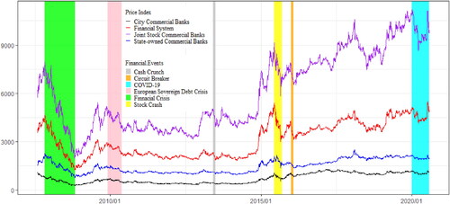
Figure 2 shows the dynamics of the commercial bank stock price index and the overall financial stock price index. Note that the commercial bank’s stock price index and overall financial stock price index have similar changing trends. Specifically, when an extreme adverse event occurred, both the commercial bank stock index and China’s financial stock index showed an extreme downward trend. Likewise, when the financial market is full of good news, the rising range of stock prices also increases. However, the reactions of different commercial banks’ stock prices to extreme shocks have been heterogeneous over time. Since the financial crisis, China’s economy has gradually recovered, but the growth rate is also gradually slowing down. These new situations provide an opportunity to study risk spillovers under the conditions of extreme market risk.

Figure 2. China’s stock price indices and financial risk events.

Source: Created by the authors.

The descriptive statistics of the daily returns for China’s commercial banks stock index and financial market stock index are reported in Table 1. The average returns are positive with high standard deviations, which imply a large dispersion in volatility. The maximum and minimum returns are almost the same because of the price limiting mechanism in the Chinese stock market. The stock returns of SOCBs, JSCBs and CCBs have positive skewness values, while those of financial systems have negative skewness values. All of the stock returns have high kurtosis values, which is in line with the properties of sharp peaks, fat tails and skewness for the return distributions. Meanwhile, we reject the hypothesis of the normality of stock returns according to the Jarque-Bera statistics.

5. Empirical results and discussion

5.1. Estimation of the marginal distribution

To shape the apparent properties of sharp peaks, fat tails and skewness of the stock returns, we chose to use the SKST distribution as the marginal distributions of the copula function. We obtained the estimated results of the return distributions by using the MLE and the associated probability density curves, as shown in Table 2 and Figure 3. The location parameter (μ), scale parameter (σ), shape parameter (ϑ) and skewness parameter (γ) together indicate that the stock returns for China’s banking sector are not normally distributed. We also tested the accuracy of the SKST distribution by drawing QQ plots of the stock returns. The results are shown in Figure 4. The scatter plots fit the line well, indicating that the estimates of SKST distribution are precise.

Figure 3. Histograms and PDFs of the stock returns.

Source: Created by the authors.

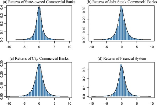
Figure 4. QQ plots of the stock returns.

Source: Created by the authors.

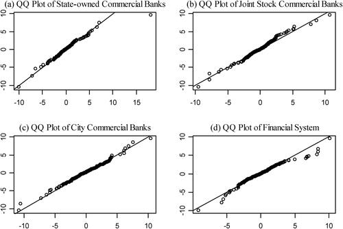
Table 2. Estimates of parameters of the SKST distribution function.

Estimates	SOCBs	JSCBs	CCBs	Financial system
$\mu$	0.0036	0.0368	0.0031	0.0390
$\sigma$	4.3278	3.0381	2.5939	2.7199
$\vartheta$	2.0734	2.3182	2.5226	2.3428
$\gamma$	1.0195	1.0495	1.0139	1.0225

Note: This table provides the MLE of the SKST distribution for stock returns of SOCBs, JSCBs, CCBs and the financial system.

Source: Authors own estimations.

5.2. Downside and upside tail dependence

The coefficients $\widehat{\delta },$ $\widehat{\theta }$ and $\widehat{\eta }$ for the Clayton and Gumbel CQR models were estimated at the 0.05 and 0.95 quantiles. The estimated results are reported in Table 3. Table 3 shows that the panning parameter $\widehat{\theta }$ is negative for the Clayton CQR model and positive for the Gumbel CQR model at the two quantiles. Furthermore, the zooming parameter $\widehat{\eta }$ is always larger than 1. These results are consistent with the fitted curves shown in Figure 5(a)–(c), where the left tail of the Clayton CQR curve is pulled down, and the right tail of the Gumbel CQR curve is pulled up. The estimated results of parameters $\widehat{\theta }$ and $\widehat{\eta }$ indicate that the CQR-based CoVaR model can better capture nonlinear tail dependence between financial returns.

Figure 5. Fitted curves of the CQR models.

Source: Created by the authors.

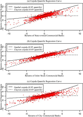
Table 3. Estimates for the CQR models.

Banks	Estimates	Clayton CQR model	Gumbel CQR model
		$\tau$=0.05	$\tau$=0.95
SOCBs	$\widehat{\delta }$	5.15*** (1.78)	9.25** (3.99)
	$\widehat{\theta }$	−0.29 (0.20)	0.96*** (0.17)
	$\widehat{\eta }$	1.18*** (0.05)	1.01*** (0.04)
JSCBs	$\widehat{\delta }$	19.45*** (4.41)	16.27*** (3.95)
	$\widehat{\theta }$	−0.63*** (0.08)	0.83*** (0.07)
	$\widehat{\eta }$	1.21*** (0.04)	1.06*** (0.03)
CCBs	$\widehat{\delta }$	8.61*** (2.32)	5.89 *** (1.68)
	$\widehat{\theta }$	−0.53*** (0.13)	0.62*** (0.18)
	$\widehat{\eta }$	1.16*** (0.04)	1.03*** (0.04)

Note: Standard errors appear in parentheses. *** and ** indicate significance levels of 1% and 5%, respectively.

Source: Authors own estimations.

According to the estimated parameter $\widehat{\delta }$ presented in Table 3, we found the values of $\widehat{\delta }$ at the 0.05 quantile to be larger than at the 0.95 quantile for JSCBs and CCBs, though the opposite is true for SOCBs. To analyse the tail-dependent structure, we also estimated the tail dependence coefficients shown in Table 4. Note that the downside tail dependence coefficients are larger than the upside tail dependence coefficients for JSCBs and CCBs, but SOCBs hold larger upside tail dependence with the financial system. This difference in tail risk dependence among the three types of commercial banks may be due to their different positions in the Chinese banking industry. The SOCBs in China are state holding and thus ‘too big to fail’. The government tends to give priority to buying SOCB stocks rather than the other two types of banks to rescue the market when the banking sector stocks plummet, which eases the downside dependence for SOCBs, to a certain extent. Finally, we found that JSCBs have the largest coefficients of downside and upside tail dependence among three kinds of commercial banks, indicating the stronger tail dependence between JSCBs and the financial system. Therefore, compared with SOCBs and CCBs, JSCBs should be the focus of risk supervision.

Table 4. Estimates of downside and upside tail dependence coefficients.

Banks	Clayton copula	Gumbel copula
SOCBs	0.8740	0.9221
JSCBs	0.9650	0.9565
CCBs	0.9227	0.8751

Note: The downside and upside tail dependence coefficients for Clayton and Gumbel copulas are computed based on $\widehat{\delta }$ in Table 3.

Source: Authors own estimations.

In summary, we find significant differences in the tail dependencies between different types of banking and financial systems. But the tail dependence indicator cannot detect the size and direction of the risk spillover into the financial system when different types of banking are in financial distress. Therefore, it is also necessary to study the risk spillover effects of commercial banks on the financial system.

5.3. Static risk spillovers from different types of commercial banks

In this subsection, we estimate and rank the static risk spillovers from the three kinds of commercial banks to the financial system. We first selected downside and upside VaRs in Table 1 as the proxy variables for downside and upside risk. We then calculated the associated downside and upside risk spillovers and risk-spillover intensity at the 0.95 confidence level.

Tables 5 and 6 show the results of the downside and upside risk spillovers. At the 0.95 confidence level, JSCBs have the largest upside and downside risk spillovers among three kinds of commercial banks at different risk levels, indicating that JSCBs contribute the largest risk to the financial system (Yang & Li, 2018). SOCBs and CCBs display the smallest upside and downside risk spillovers, respectively. Though the market share of SOCBs is much larger than that of JSCBs, the risk spillovers from JSCBs are higher than those of SOCBs. This finding also indicates that scale is not necessarily the key factor determining whether a specific type of commercial bank is systemically important. Similarly, we found the downside risk of SOCBs, measured by their VaR, to be smaller than that of CCBs (see Table 1). However, the downside risk spillovers from SOCBs were larger than those from CCBs. This finding reveals that the higher risk level of one financial institution does not mean that it has a higher spillover effect on the financial system.

Table 5. Static risk spillovers of downside risk.

Banks	Estimates	$\alpha$=1%	$\alpha$=2%	$\alpha$=3%	$\alpha$=4%	$\alpha$=5%	$\alpha$=6%	$\alpha$=7%	$\alpha$=8%	$\alpha$=9%	$\alpha$=10%
SOCBs	${\mathit{DCoVaR}}_{0.05}^{s|{\mathit{VaR}}_{0.5}^i}$	−0.95	−0.95	−0.95	−0.95	−0.95	−0.95	−0.95	−0.95	−0.95	−0.95
	$D{\mathit{CoVaR}}_{0.05}^{s|{\mathit{VaR}}_{\alpha }^i}$	−7.93	−6.46	−5.67	−5.00	−4.48	−4.13	−3.84	−3.60	−3.41	−3.20
	$\Delta \mathit{DCoVaR}$	−6.98	−5.51	−4.72	−4.05	−3.52	−3.17	−2.89	−2.65	−2.45	−2.24
	$\mathrm{\%}\mathit{DCoVaR}$	731.79%	577.76%	494.45%	424.53%	369.55%	332.49%	302.82%	277.37%	257.32%	235.02%
JSCBs	${\mathit{DCoVaR}}_{0.05}^{s|{\mathit{VaR}}_{0.5}^i}$	−0.86	−0.86	−0.86	−0.86	−0.86	−0.86	−0.86	−0.86	−0.86	−0.86
	$D{\mathit{CoVaR}}_{0.05}^{s|{\mathit{VaR}}_{\alpha }^i}$	−8.13	−6.31	−5.34	−4.70	−4.24	−3.98	−3.71	−3.49	−3.27	−3.10
	$\Delta \mathit{DCoVaR}$	−7.27	−5.45	−4.48	−3.84	−3.37	−3.11	−2.85	−2.63	−2.40	−2.24
	$\mathrm{\%}\mathit{DCoVaR}$	840.63%	630.60%	517.79%	444.23%	390.32%	360.10%	329.44%	304.12%	278.13%	258.67%
CCBs	${\mathit{DCoVaR}}_{0.05}^{s|{\mathit{VaR}}_{0.5}^i}$	−0.97	−0.97	−0.97	−0.97	−0.97	−0.97	−0.97	−0.97	−0.97	−0.97
	$D{\mathit{CoVaR}}_{0.05}^{s|{\mathit{VaR}}_{\alpha }^i}$	−7.96	−6.25	−5.18	−4.68	−4.33	−4.06	−3.78	−3.50	−3.33	−3.09
	$\Delta \mathit{DCoVaR}$	−7.00	−5.29	−4.22	−3.72	−3.37	−3.10	−2.82	−2.54	−2.36	−2.12
	$\mathrm{\%}\mathit{DCoVaR}$	725.12%	547.60%	436.95%	385.36%	349.01%	321.09%	292.08%	262.68%	244.57%	219.92%

Note: ${\mathit{DCoVaR}}_{0.05}^{s|{\mathit{VaR}}_{0.5}^i}$ and $D{\mathit{CoVaR}}_{0.05}^{s|{\mathit{VaR}}_{\alpha }^i}$ denote the downside CoVaR of financial system condition on the normal state and financial distress with different risk levels. Financial distress is measured as the return of banking taking values equal to its VaR. $\alpha$ denotes the risk level of financial event. For example, $\alpha =1\%$ means a financial event once in 100 years. $\Delta \mathit{DCoVaR}$ and$\%\mathit{DCoVaR}$ are downside risk spillovers and risk-spillover intensity computed according to Equations (16)(16) $${\Delta \mathit{DCoVaR}}_{\beta }^{s|i}{=\mathit{DCoVaR}}_{\beta }^{s|X^i={\mathit{VaR}}_{\alpha }^i}-{\mathit{DCoVaR}}_{\beta }^{s|X^i={\mathit{VaR}}_{0.5}^i},\mathrm{ }$$(16) and (18)(18) $$\mathrm{\%}{\mathit{DCoVaR}}_{\beta }^{s|i}=({\Delta \mathit{DCoVaR}}_{\beta }^{s|i}/{\mathit{DCoVaR}}_{\beta }^{s|X^i={\mathit{VaR}}_{0.5}^i})\mathrm{*}100\mathrm{\%},$$(18) .

Source: Authors own estimations.

Table 6. Static risk spillovers of upside risk.

	Estimates	$\alpha$=90%	$\alpha$=91%	$\alpha$=92%	$\alpha$=93%	$\alpha$=94%	$\alpha$=95%	$\alpha$=96%	$\alpha$=97%	$\alpha$=98%	$\alpha$=99%
SOCBs	${\mathit{UCoVaR}}_{0.95}^{s|{\mathit{VaR}}_{0.5}^i}$	1.28	1.28	1.28	1.28	1.28	1.28	1.28	1.28	1.28	1.28
	$U{\mathit{CoVaR}}_{0.95}^{s|{\mathit{VaR}}_{\alpha }^i}$	3.30	3.49	3.62	3.85	4.12	4.47	4.89	5.42	6.06	7.48
	$\Delta \mathit{UCoVaR}$	2.02	2.20	2.34	2.57	2.84	3.18	3.61	4.13	4.78	6.20
	$\mathrm{\%}\mathit{UCoVaR}$	157.07%	171.32%	181.86%	199.65%	221.00%	247.68%	280.95%	321.74%	371.94%	482.47%
JSCBs	${\mathit{UCoVaR}}_{0.95}^{s|{\mathit{VaR}}_{0.5}^i}$	1.01	1.01	1.01	1.01	1.01	1.01	1.01	1.01	1.01	1.01
	$U{\mathit{CoVaR}}_{0.95}^{s|{\mathit{VaR}}_{\alpha }^i}$	3.14	3.31	3.46	3.71	3.92	4.19	4.66	5.33	6.09	7.25
	$\Delta \mathit{UCoVaR}$	2.13	2.30	2.44	2.70	2.91	3.18	3.65	4.32	5.08	6.24
	$\mathrm{\%}\mathit{UCoVaR}$	210.02%	226.87%	241.32%	266.20%	287.31%	313.73%	360.21%	426.25%	501.14%	615.84%
CCBs	${\mathit{UCoVaR}}_{0.95}^{s|{\mathit{VaR}}_{0.5}^i}$	1.11	1.11	1.11	1.11	1.11	1.11	1.11	1.11	1.11	1.11
	$U{\mathit{CoVaR}}_{0.95}^{s|{\mathit{VaR}}_{\alpha }^i}$	3.24	3.43	3.58	3.80	4.05	4.30	4.83	5.44	6.56	8.67
	$\Delta \mathit{UCoVaR}$	2.13	2.32	2.47	2.69	2.94	3.19	3.72	4.33	5.45	7.56
	$\mathrm{\%}\mathit{UCoVaR}$	191.59%	209.16%	222.03%	242.14%	264.95%	287.21%	334.59%	389.87%	490.54%	680.53%

Note: ${\mathit{UCoVaR}}_{0.95}^{s|{\mathit{VaR}}_{0.5}^i}$ and $U{\mathit{CoVaR}}_{0.95}^{s|{\mathit{VaR}}_{\alpha }^i}$ denote the upside CoVaR of financial system condition on the normal state and financial distress with different risk levels. Financial distress is measured as the return of banking taking values equal to its VaR. $\alpha$ denotes the risk level of financial event. For example, $\alpha =95\%$ means a financial event once in 20 years. $\Delta \mathit{UCoVaR}$ and $\%\mathit{UCoVaR}$ are upside risk spillovers and risk-spillover intensity computed according to Equations (17)(17) $${\Delta \mathit{UCoVaR}}_{1-\beta }^{s|i}{=\mathit{UCoVaR}}_{1-\beta }^{s|X^i={\mathit{VaR}}_{1-\alpha }^i}-{\mathit{UCoVaR}}_{1-\beta }^{s|X^i={\mathit{VaR}}_{0.5}^i},$$(17) and (19)(19) $$\mathrm{\%}{\mathit{UCoVaR}}_{1-\beta }^{s|i}=({\Delta \mathit{UCoVaR}}_{1-\beta }^{s|i}/{\mathit{UCoVaR}}_{1-\beta }^{s|X^i={\mathit{VaR}}_{0.5}^i})\mathrm{*}100\mathrm{\%}.$$(19) .

Source: Authors own estimations.

On average SOCBs, JSCBs and CCBs held more than 73% of all NPLs from 2016 to 2018. Specifically, SOCBs held a greater number of NPLs than JSCBs and CCBs, indicating the highest financial risk in the three kinds of commercial banks. However, we also found the risk spillovers from SOCBs into the financial system to be smaller than those from JSCBs, which implies that NPLs are not necessarily the only determinant factor for whether a bank is systemically important. The possible reason behind this finding is that SOCBs are often backed by state credit, leading market participants to generally expect these banks to be ‘too big to fail’. That is, when these commercial banks are in distress due to a high level of NPLs, the government will provide assistance, so their solvency and, therefore, their stability will not be affected. However, JSCBs lack the credit support from the state that SOCBs enjoy.

Furthermore, the downside risk-spillover intensity of SOCBs, JSCBs and CCBs ranges from 219.92% to 840.63%, but the upside risk-spillover intensity ranges from 157.07% to 680.53%. This significant difference indicates that the risk spillovers are asymmetric, with a much smaller upside than downside spillovers. This finding is in line with the flight-to-quality phenomenon. That is, there is an asymmetric reaction of capital flows triggered by upside and downside risk, with these capital flows amplifying upside risk spillovers to a smaller extent than downside risk spillovers (Reboredo et al., 2016).

5.4. Dynamic risk spillovers from different types of commercial banks

In this subsection, we quantify the dynamic spillovers of downside risk and upside risk from the three kinds of commercial banks into the financial system using the dynamic rolling CoVaR model. Here, we set $n_0$ to 1,781 and $l$ to 1, and we obtain 997-day rolling windows $T_1,T_2\cdots T_{997}$ from 2 December 2014 to 31 July 2020. Based on these rolling windows, the downside and upside risk-spillover intensity can be computed to characterise the dynamic risk spillovers at different time points. The results are reported in Figures 6 and 7.

Figure 6. The dynamics of downside risk spillovers from the three kinds of banks to financial system in China over period from 2 December 2014 to 31 July 2020.

Source: Created by the authors.

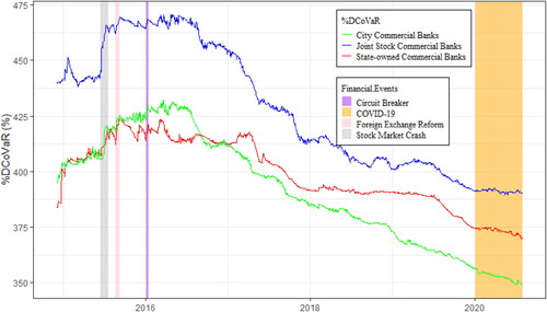
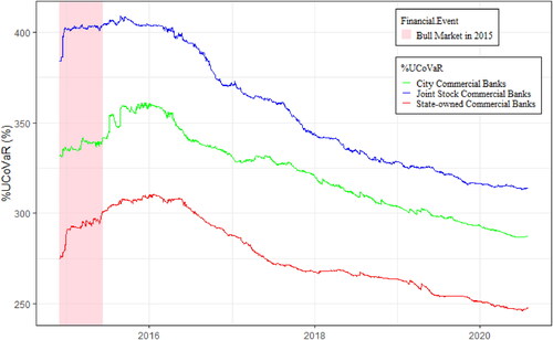
Figure 7. The dynamics of upside risk spillovers from the three kinds of banks to financial system in China from 2 December 2014 to 31 July 2020.

Source: Created by the authors.

According to the downside spillovers in Figure 6, we find that the downside spillovers rose rapidly to a high level and remained so for a long time since the Chinese stock market crash, from 15 June 2015 to mid-2016. Moreover, we also find the dynamic spillovers are sensitive to extreme negative events, such as the stock market crash of June 2015, the so-called 8.11 foreign exchange reform of 2015 and the new ‘circuit breaker’ mechanism implemented in early 2016. Finally, we explore the risk spillover of the banking sector since the COVID-19 epidemic spread globally starting from January 2020. We find that the downward trend of downside risk spillovers from JSCBs and SOCBs into the financial system rose at beginning of the pandemic. However, the downside risk spillovers remain stable as China takes some policies to control these risks, which are possibly caused by this epidemic. For example, the People’s Bank of China has provided 300 billion yuan in low-cost special reloan funds to major national banks and some local corporate banks in key provinces during the epidemic periods. Its utility in doing this is in easing the credit constraints in the banking sector.

Based on the upside risk spillovers in Figure 7, we find that they are higher than 275% on average, which provides clear evidence of upside risk spillovers sourced from the commercial banks. Moreover, JSCBs display the largest upside risk spillovers. This finding is in line with the results in Table 6. We also find that the upside spillovers from these three types of banks increase gradually and peak when the stock market is bullish. For example, we find that, between 2014 and 12 June 2015, the upside spillovers from JSCBs, SOCBs and CCBs gradually increased and became higher than that in other periods.

In summary, we find the upside and downside risk spillovers of JSCBs to be the highest and the upside risk spillovers of SOCBs and downside risk spillovers of CCBs to be the smallest, findings which are consistent with the studies by Wang et al. (2017, 2018), who also found that SOCBs contribute less to volatility connectedness than JSCBs and CCBs. The results of the dominance test in Table 7 corroborate this conclusion. The findings from Figures 6 and 7 indicate that dynamic risk spillovers can be a useful instrument for understanding how financial shocks are transmitted from commercial banks to the financial system.

Table 7. Dominance tests for the risk spillovers.

	Null hypothesis	Statistics	p-Value
Downside	$H_0:\mathrm{SOCBs }\mathrm{\ge }\mathrm{JSCBs}$	0.508	0.000***
	$H_0:C\mathrm{CBs}\ge JS\mathrm{CBs}$	0.503	0.000***
	$H_0:C\mathrm{CBs}\ge SO\mathrm{CBs}$	1	0.000***
Upside	$H_0:\mathrm{SOCBs }\mathrm{\ge }\mathrm{JSCBs}$	0.473	0.000***
	$H_0:C\mathrm{CBs}\ge JS\mathrm{CBs}$	0.508	0.000***
	$H_0:\mathrm{SOCBs}\ge \mathit{CCBs}$	0.503	0.000***

Note: The null hypothesis ‘SOCBs ≥ JSCBs’ means that the SOCBs are more or equally risky than the JSCBs when financial events with the same risk levels occur in these two kinds of commercial banks. Three asterisks indicate significance at the 1% level.

Source: Authors own estimations.

In addition, to assess whether one kind of commercial bank is significantly risky for the entire financial system, we implemented the significance test for the dynamic risk spillovers using bootstrap KS tests. The significance statistics and p-values are shown in Table 8. Note that the p-value of the significance statistics for risk spillovers is equal to 0, indicating that the downside and upside risks spillovers are significant at the 1% confidence level.

Table 8. Significance tests for the risk spillovers.

	Null hypothesis	Statistics	p-Value
Downside	$H_0:\Delta \mathit{DCoVaR}\mathit{\text{ of }}\mathrm{SOCBs}=0$	1	0.000***
	$H_0:\Delta \mathit{DCoVaR}\mathit{\text{ of }}\mathrm{JSCBs}=0$	1	0.000***
	$H_0:\Delta \mathit{DCoVaR}\mathit{\text{ of }}\mathrm{CCBs}=0$	1	0.000***
Upside	$H_0:\Delta \mathit{UCoVaR}\mathit{\text{ of }}\mathrm{SOCBs}=0$	1	0.000***
	$H_0:\Delta \mathit{UCoVaR}\mathit{\text{ of }}\mathrm{JSCBs}=0$	1	0.000***
	$H_0:\Delta \mathit{UCoVaR}\mathit{\text{ of }}\mathrm{CCBs}=0$	1	0.000***

Note: Three asterisks indicate significance at the 1% level.

Source: Authors own estimations.

Finally, the asymmetry test results in Table 9 indicate that the upside risk spillovers are smaller than the downside risk spillovers, suggesting that the financial system may suffer more severely when any type of commercial bank faces downside risk.

Table 9. Asymmetry tests for the risk spillovers from banks to China’s financial system.

Banks	Null hypothesis	Statistics	p-Value
SOCBs	$H_0:\%\mathit{UCoVaR}\ge \%\mathit{DCoVaR}$	1	0.000***
JSCBs	$H_0:\%\mathit{UCoVaR}\ge \%\mathit{DCoVaR}$	0.707	0.000***
CCBs	$H_0:\%\mathit{UCoVaR}\ge \%\mathit{DCoVaR}$	0.868	0.000***

Note: Three asterisks indicate significance at the 1% level.

Source: Authors own estimations.

6. Policy implications

Our findings have important policy implications for financial regulators and investors. Firstly, our findings have important guiding significance for the financial risk supervision department. We find the JSCBs, not the SOCBs, have the largest upside and downside risk spillovers, indicating that for the banking regulators, when identifying SIBs, they should consider not only a bank’s size, NPLs and VaR but also their risk spillovers. Thus, a scientific assessment mechanism based on risk spillover should be established to capture the truly important banks in the financial market accurately. Furthermore, it also indicates that the regulatory authorities can take their eyes away from SOCBs and should pay more attention to the risk level of JSCBs and their impacts on China’s financial system in the long run. At the same time, regulatory authorities can issue related risk management policies and establish a long-term risk early warning mechanism for JSCBs.

Besides, our findings can inspire investors to optimise their investment strategies. This paper shows that investors can track the risk evolution of China’s financial market by observing the risk of JSCBs mainly and then adjusting their investment strategies. For example, the asymmetric risk spillovers, with downside risk spillovers larger than upside risk spillovers, indicate that the fund managers with long positions in the financial industry will face larger risk during the times of bearish stock market than those with short positions during the periods of bullish stock market. Thus, fund managers should consider the asymmetric features of risk contagions and accordingly hedge and adjust their positions to optimise portfolios strategy. Moreover, the higher downside risk spillovers from the JSCBs indicate that portfolio managers with long positions in the financial industry will face greater risk during periods when the JSCBs are under distress than during periods when SOCBs and CCBs experience prices fall. Thus, fund managers should close their long positions or allocate proper instruments to hedge the risk spillovers on time when steep falls in three types of commercial banks begin, especially in the JSCBs. The economic implications of upside risk spillovers are similar to that for downside risk spillovers, but short positions are considered instead of long positions.

7. Conclusions

Systemic risk in the Chinese banking industry has increased dramatically in recent years due to the rapid expansion of credit and the high number of NPLs held by commercial banks. Therefore, it is urgent to investigate the risk spillovers from the banking sector into the financial system. Most conventional models used to compute CoVaR often ignore the nonlinearity of tail dependence structure among different financial variables. To addresses this issue, we proposed a new CQR-based CoVaR model. Using this newly proposed model, we have measured static and dynamic risk spillovers from three types of commercial banks into the financial system in China. We found that the risk spillovers exhibit time-varying heterogeneity and that the downward trend is significant after the onset of the stock market disaster from 15 June 2015 to mid-2016. We also found that JSCBs have the largest risk spillovers and are therefore the main contributors to systemic financial risk in the banking sector and should be the main target of subsequent regulation. Finally, we found that the risk spillovers are asymmetric, a finding which is consistent with the flight-to-quality phenomenon.

The generalisability of the empirical results is subject to certain limitations. For instance, the policy implications in this paper are not applicable to other economies due to the differences in economic environment and conditions in different countries. Furthermore, the empirical results are mainly based on daily data. However, daily data has more noise than weekly and monthly data, which may affect the accuracy of the results. In spite of its limitations, the study certainly adds to our understanding of the role the banking sector has played in the overall financial system in China.

In future, our research can be extended in two directions. First, different risk measures can be introduced into our model. In this study, the CoVaR is selected to measure systemic risk, which is not a coherent risk measure if the financial variables follow the SKST distribution. Therefore, we can use the coherent risk measures such as CoES for exploring the systemic financial risk under the more complicated scenario which can present the real financial market situation. Second, this highly data-driven framework for computing risk spillovers can be widely used as a monitoring device in the field of risk management. For example, it can be used to identify not only SIBs but also systemically important financial institutions. The risk spillovers calculated under this framework provide a market view on the downside and upside risk co-movements in financial markets.

Disclosure statement

No potential conflict of interest was reported by the authors.

Additional information

Funding

This research was supported by the National Natural Science Foundation of China (Nos. 72173096, 71873103, 71731003, 72101120), the Humanities and Social Sciences project of the Ministry of Education of China (No. 18YJC910011), the Chinese Universities Scientific Fund (No. 2452021189), the Social Science Foundation of Shaanxi Province, China (No. 2018D51), and the Innovation Capability Support Program of Shaanxi (No. 2019KJXX-070). Shi acknowledges the financial support from the Tang Scholar Program of Northwest A&F University, China (No. 2021-04).

Appendix A.

Simulations of the Clayton and Gumbel CQR functions

The Clayton and Gumbel CQR functions can accurately capture the nonlinearity of downside and upside tail dependence between financial variables, respectively. To illustrate this desirable property, we draw 1,000 random values of ($X,Y$) and depict 5 simulated curves for the Clayton and Gumbel CQR functions at quantiles 0.05, 0.25, 0.5, 0.75 and 0.95. Specifically, the Clayton CQR curves under the hypothesis of SKST margins ($X\sim \mathit{SKST}\left(0,1.5,4,0.8\right),Y\sim \mathit{SKST}\left(0,2,3,1.1\right)$) for $\delta =3$ are shown in Figure A1(a), which indicates that the Clayton CQR function cannot properly describe the upside tail dependence but does capture the downside tail dependence of $X$ and $Y.$

Figure A1. Clayton and Gumbel CQR curves.

Source: Created by the authors.

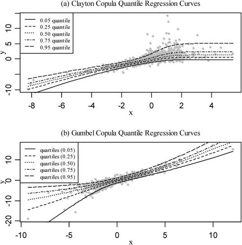
Similarly, the Gumbel CQR curves under the hypothesis of SKST margins ($X\sim \mathit{SKST}\left(0,2,4,1.2\right),\mathrm{ }Y\sim \mathit{SKST}\left(0,3,3,1.1\right)$) for $\delta =3$ are shown in Figure A1(b). It is obvious that the Gumbel CQR function cannot capture the downside tail dependence but does trace the upside tail dependence of $X$ and $Y.$

Appendix B.

The significance, dominance and asymmetry tests

To determine whether one type of commercial bank contributes significantly to the entire financial system, we employ the two-sample bootstrap KS test (Abadie, 2002) to compare the cumulative distribution functions (CDFs) of the dynamics of benchmark CoVaR and CoVaR. The associated statistic of the significance test is defined as follows: $$D_{mn}{=\left(mn/(m+n)\right)}^{0.5}sup\left|F_m\left(x\right)-G_n\left(x\right)\right|,$$ where $F_m(x)$ and $G_n(x)$ are the CDFs of the dynamics of benchmark CoVaR and CoVaR, respectively, and m and n represent the size of the two samples. The null hypotheses of downside and upside spillovers are defined as follows: $$H_0:\Delta D{\mathit{CoVaR}}_{0.05}^{s|i}={\mathit{DCoVaR}}_{0.05}^{s|{\mathit{VaR}}_{0.05}^i}-{\mathit{DCoVaR}}_{0.05}^{s|{\mathit{VaR}}_{0.5}^i}=0,$$ and $$H_0:\Delta U{\mathit{CoVaR}}_{0.95}^{s|i}={\mathit{UCoVaR}}_{0.95}^{s|{\mathit{VaR}}_{0.95}^i}-U{\mathit{CoVaR}}_{0.95}^{s|{\mathit{VaR}}_{0.5}^i}=0.$$

Similarly, to determine whether commercial banks of type $i$ contribute less to the financial system than type $j,$ we use the two-sample bootstrap KS test to compare the CDFs of the dynamics of %CoVaR and benchmark %CoVaR. The stochastic dominance statistic is defined as follows: $$D_{mn}{=\left(mn/(m+n)\right)}^{0.5}sup\left|A_m\left(x\right)-B_n\left(x\right)\right|,$$ where $A_m(x)$ and $B_n(x)$ represent the CDFs of the dynamics of %CoVaR and benchmark %CoVaR, respectively. The null hypotheses of the downside and upside risk-spillover intensity are defined as follows: $$H_0:\mathrm{\%}D{\mathit{CoVaR}}_{0.05}^{s|j}\ge \mathrm{\%}D{\mathit{CoVaR}}_{0.05}^{s|i},$$ and $$H_0:\mathrm{\%}U{\mathit{CoVaR}}_{0.95}^{s|j}\ge \mathrm{\%}U{\mathit{CoVaR}}_{0.95}^{s|i}.$$

Finally, the asymmetry tests can assess whether the upside spillover of one type of commercial bank contributes more to the financial system than the downside spillover. The asymmetry test can also be implemented by the two-sample bootstrap KS test. The null hypothesis is defined as follows: $$H_0:\mathrm{\%}U{\mathit{CoVaR}}_{0.95}^{s|i}\ge \mathrm{\%}D{\mathit{CoVaR}}_{0.05}^{s|i}.$$

References

- Abadie, A. (2002). Bootstrap tests for distributional treatment effects in instrumental variable models. Journal of the American Statistical Association, 97(457), 284–292. https://doi.org/10.1198/016214502753479419
- Acharya, V., Engle, R., & Richardson, M. (2012). Capital shortfall: A new approach to ranking and regulating systemic risks. American Economic Review, 102(3), 59–64. https://doi.org/10.1257/aer.102.3.59
- Acharya, V., Pedersen, L. H., Philippon, T., & Richardson, M. (2017). Measuring systemic risk. Review of Financial Studies, 30(1), 2–47. https://doi.org/10.1093/rfs/hhw088
- Adams, Z., Füss, R., & Gropp, R. (2014). Spillover effects among financial institutions: A state-dependent sensitivity value-at-risk approach. Journal of Financial and Quantitative Analysis, 49(3), 575–598. https://doi.org/10.1017/S0022109014000325
- Adrian, T., & Brunnermeier, M. K. (2016). CoVaR. American Economic Review, 106(7), 1705–1741. https://doi.org/10.1257/aer.20120555
- Ameur, H. B., Jawadi, F., Jawadi, N., & Cheffou, A. I. (2020). Assessing downside and upside risk spillovers across conventional and socially responsible stock markets. Economic Modelling, 88, 200–210. https://doi.org/10.1016/j.econmod.2019.09.023
- Bernal, O., Gnabo, J. Y., & Guilmin, G. (2014). Assessing the contribution of banks, insurance and other financial services to systemic risk. Journal of Banking & Finance, 47, 270–287. https://doi.org/10.1016/j.jbankfin.2014.05.030
- Bernardi, M., Maruotti, A., & Petrella, L. (2017). Multiple risk measures for multivariate dynamic heavy-tailed models. Journal of Empirical Finance, 43, 1–32. https://doi.org/10.1016/j.jempfin.2017.04.005
- Billio, M., Getmansky, M., Lo, A. W., & Pelizzon, L. (2012). Econometric measures of connectedness and systemic risk in the finance and insurance sectors. Journal of Financial Economics, 104(3), 535–559. https://doi.org/10.1016/j.jfineco.2011.12.010
- Bisias, D., Flood, M. D., Lo, A. W., & Valavanis, S. (2012). A survey of systemic risk analytics. U.S. Department of Treasury, Office of Financial Research No. 0001, https://ssrn.com/abstract=1983602 or https://doi.org/10.2139/ssrn.1983602.
- Borri, N., & Giorgio, G. D. (2022). Systemic risk and the COVID challenge in the European banking sector. Journal of Banking & Finance, 140, 106073. https://doi.org/10.1016/j.jbankfin.2021.106073
- Bouyé, E., & Salmon, M. (2009). Dynamic copula quantile regressions and tail area dynamic dependence in forex markets. The European Journal of Finance, 15(7-8), 721–750. https://doi.org/10.1080/13518470902853491
- Brownlees, C., & Engle, R. (2017). SRISK: A conditional capital shortfall measure of systemic risk. Review of Financial Studies, 30(1), 48–79. https://doi.org/10.1093/rfs/hhw060
- Charpentier, A., & Segers, J. (2007). Lower tail dependence for Archimedean copulas: Characterizations and pitfalls. Insurance: Mathematics and Economics, 40(3), 525–532.
- Dell’Ariccia, G., Igan, D., Laeven, L., & Tong, H. (2016). Credit booms and macrofinancial stability. Economic Policy, 31(86), 299–355. https://doi.org/10.1093/epolic/eiw002
- Fan, X. Q., Du, M. D., & Long, W. (2017). Risk spillover effect of Chinese commercial banks: Based on indicator method and CoVAR approach. Procedia Computer Science, 122, 932–940. https://doi.org/10.1016/j.procs.2017.11.457
- Ghulam, Y., & Doering, J. (2018). Spillover effects among financial institutions within Germany and the United Kingdom. Research in International Business and Finance, 44, 49–63. https://doi.org/10.1016/j.ribaf.2017.03.004
- Girardi, G., & Ergün, A. (2013). Systemic risk measurement: Multivariate GARCH estimation of CoVaR. Journal of Banking & Finance, 37(8), 3169–3180. https://doi.org/10.1016/j.jbankfin.2013.02.027
- Glasserman, P., & Young, P. (2015). How likely is contagion in financial networks? Journal of Banking & Finance, 50, 383–399. https://doi.org/10.1016/j.jbankfin.2014.02.006
- Ji, Q., Liu, B., & Fan, Y. (2019). Risk dependence of CoVaR and structural change between oil prices and exchange rates: A time-varying copula model. Energy Economics, 77, 80–92. https://doi.org/10.1016/j.eneco.2018.07.012
- Ji, Q., Liu, B. Y., Zhao, W. L., & Fan, Y. (2020). Modelling dynamic dependence and risk spillover between all oil price shocks and stock market returns in the BRICS. International Review of Financial Analysis, 68, 101238. https://doi.org/10.1016/j.irfa.2018.08.002
- Karimalis, E. N., & Nomikos, N. K. (2018). Measuring systemic risk in the European banking sector: A copula CoVaR approach. The European Journal of Finance, 24(11), 944–975. https://doi.org/10.1080/1351847X.2017.1366350
- Koenker, R. (2005). Quantile regression. Cambridge University Press.
- Kolari, J. W., Lopez-Iturriaga, F. J., & Sanz, I. P. (2020). Measuring systemic risk in the US Banking system. Economic Modelling, 91, 646–658. https://doi.org/10.1016/j.econmod.2019.12.005
- Laeven, L., Ratnovski, L., & Tong, H. (2016). Bank size, capital, and systemic risk: Some international evidence. Journal of Banking & Finance, 69, S25–S34. https://doi.org/10.1016/j.jbankfin.2015.06.022
- Lin, E. M. H., Sun, E. W., & Yu, M. T. (2018). Systemic risk, financial markets, and performance of financial institutions. Annals of Operations Research, 262(2), 579–603. https://doi.org/10.1007/s10479-016-2113-8
- López-Espinosa, G., Moreno, A., Rubia, A., & Valderrama, L. (2015). Systemic risk and asymmetric responses in the financial industry. Journal of Banking & Finance, 58(152), 471–485. https://doi.org/10.1016/j.jbankfin.2015.05.004
- Medina-Olivares, V., Calabrese, R., Dong, Y. Z., & Shi, B. F. (2022). Spatial dependence in microfinance credit default. International Journal of Forecasting, 38(3), 1071–1085. https://doi.org/10.1016/j.ijforecast.2021.05.009
- Nelsen, R. B. (2006). An introduction to copulas (2nd ed.). Springer.
- Ouyang, Z. S., Huang, Y., Jia, Y., & Luo, C. Q. (2020). Measuring systemic risk contagion effect of the banking industry in China: A directed network approach. Emerging Markets Finance and Trade, 56(6), 1312–1335. https://doi.org/10.1080/1540496X.2019.1711368
- Pham, T. N., Powell, R., & Bannigidadmath, D. (2021). Systemically important banks in Asian emerging markets: Evidence from four systemic risk measures. Pacific-Basin Finance Journal, 70, 101670. https://doi.org/10.1016/j.pacfin.2021.101670
- Raffestin, L. (2014). Diversification and systemic risk. Journal of Banking & Finance, 46, 85–106. https://doi.org/10.1016/j.jbankfin.2014.05.014
- Reboredo, J., & Ugolini, A. (2015). Systemic risk in European sovereign debt markets: A CoVaR-copula approach. Journal of International Money and Finance, 51(3), 214–244. https://doi.org/10.1016/j.jimonfin.2014.12.002
- Reboredo, J., Rivera-Castro, M., & Ugolini, A. (2016). Downside and upside risk spillovers between exchange rates and stock prices. Journal of Banking & Finance, 62, 76–96. https://doi.org/10.1016/j.jbankfin.2015.10.011
- Roukny, T., Battiston, S., & Stiglitz, J. E. (2018). Interconnectedness as a source of uncertainty in systemic risk. Journal of Financial Stability, 35(4), 93–106. https://doi.org/10.1016/j.jfs.2016.12.003
- Sun, Y., Chai, N. N., Dong, Y. Z., & Shi, B. F. (2022). Assessing and predicting small industrial enterprises’ credit ratings: A fuzzy decision making approach. International Journal of Forecasting, 38(3), 1158–1172. https://doi.org/10.1016/j.ijforecast.2022.01.006
- Teply, P., & Kvapilikova, I. (2017). Measuring systemic risk of the US banking sector in time-frequency domain. Journal of Economics and Finance, 42, 461–472.
- Tiwari, A. K., Jena, S. K., Kumar, S., & Hille, E. (2022). Is oil price risk systemic to sectoral equity markets of an oil importing country? Evidence from a dependence-switching copula delta CoVaR approach. Annals of Operations Research, 315(1), 429–461. https://doi.org/10.1007/s10479-021-04218-6
- Wang, G. J., Xie, C., He, K., & Stanley, H. E. (2017). Extreme risk spillover network: Application to financial institutions. Quantitative Finance, 17(9), 1417–1433. https://doi.org/10.1080/14697688.2016.1272762
- Wang, G. J., Xie, C., Zhao, L. F., & Jiang, Z. Q. (2018). Volatility connectedness in the Chinese banking system: Do state-owned commercial banks contribute more? Journal of International Financial Markets, Institutions & Money, 57, 205–230. https://doi.org/10.1016/j.intfin.2018.07.008
- Warshaw, E. (2019). Extreme dependence and risk spillovers across North American equity markets. The North American Journal of Economics and Finance, 47, 237–251. https://doi.org/10.1016/j.najef.2018.12.012
- Xiao, Y. (2020). The risk spillovers from the Chinese stock market to major East Asian stock markets: A MSGARCH-EVT-copula approach. International Review of Economics & Finance, 65, 173–186. https://doi.org/10.1016/j.iref.2019.10.009
- Xu, Q., Chen, L., Jiang, C., & Jing, Y. (2018). Measuring systemic risk of the banking industry in China: A DCC-MIDAS-t approach. Pacific-Basin Finance Journal, 51, 13–31. https://doi.org/10.1016/j.pacfin.2018.05.009
- Xu, Q., Jin, B., & Jiang, C. (2021). Measuring systemic risk of the Chinese banking industry: A wavelet-based quantile regression approach. The North American Journal of Economics and Finance, 55, 101354. https://doi.org/10.1016/j.najef.2020.101354
- Yang, J., Yu, Z. L., & Ma, J. (2019). China’s financial network with international spillovers: A first look. Pacific-Basin Finance Journal, 58, 101222. https://doi.org/10.1016/j.pacfin.2019.101222
- Yang, K., Wei, Y., Li, S. W., & He, J. M. (2020). Asymmetric risk spillovers between Shanghai and Hong Kong stock markets under China’s capital account liberalization. The North American Journal of Economics and Finance, 51, 101100. https://doi.org/10.1016/j.najef.2019.101100
- Yang, Z., & Li, D. (2018). An investigation of the systemic risk of Chinese banks: An application based on leave-one-out. Economic Research, 8, 36–51.
- Ye, J., Zhang, A., & Dong, Y. (2019). Banking reform and industry structure: Evidence from China. Journal of Banking & Finance, 104, 70–84. https://doi.org/10.1016/j.jbankfin.2019.05.004
- Zhu, X. (2021). The varying shadow of China’s banking system. Journal of Comparative Economics, 49(1), 135–146. https://doi.org/10.1016/j.jce.2020.07.006