Can jumps improve the futures margin level? An empirical study based on an SE-SVCJ-GPD model

Abstract

In addition to the characteristics of leptokurtic fat-tailed distribution, financial sequences also exhibit typical volatility and jumps. Moreover, jumps exhibit self-exciting and clustering characteristics under extreme events. However, studies on dynamic margin levels often ignore jumps. In this study, we combine the self-exciting stochastic volatility with correlated jumps (SE-SVCJ) model with a generalized Pareto distribution (GPD) to measure the optimal margin level for the stock index futures market. Value at risk (VaR) is estimated and forecasted using the SE-SVCJ-GPD, SVCJ-GPD, and generalized autoregressive conditional heteroskedasticity with GPD (GARCH-GPD) models. SE-SVCJ-GPD can undertake more risks in the long or short trading position of stock index futures contracts. Moreover, the backtesting experiment results show that the SE-SVCJ-GPD model provides a more accurate margin level forecast than the other methods in both positions. This study’s findings have practical significance and theoretical value for assessing the level of risk and taking corresponding risk-prevention measures.

Keywords:

• Futures margin level
• jump
• self-exciting
• generalized Pareto distribution
• value at risk

JEL CODES:

• C40
• C45
• C53

1. Introduction

Extreme events, such as the Asian financial crisis, the subprime mortgage crisis in the United States, and the global COVID-19 pandemic, have a significant effect on the global financial market (Goodell, 2020; Iglesias, 2022), and investors have become more concerned about market risk (Mansor et al., 2019). Stock index futures are products based on stock market indices. As an important investment tool in the capital market, futures products have many advantages such as hedging, reducing spot volatility, and improving transaction quality. Investors are required to pay a certain percentage of deposits to futures exchanges when trading stock index futures as a financial guarantee for the performance of the futures contracts. However, setting the margin level creates a dilemma: how should market liquidity and the probability of default be balanced? If the margin level is set too high, the investors’ opportunity cost will increase, which causes less market liquidity and a lower probability of default risk. If the margin level is set too low, the investors’ opportunity cost will decrease, which causes more market liquidity and a larger probability of default risk. Therefore, academia has devoted much time to exploring more accurate margin level forecasts in their exploration of management risk.

The traditional characteristics of financial time series, such as leptokurtic fat-tailed distribution, asymmetry, and bias, are well known. GARCH or SV models describe these properties well. However, numerous studies have confirmed the importance of jumps (Akgiray & Booth, 1988, Tucker & Pond, 1988, Hsieh, 1989). In existing research, the common treatment method combines the jump structure with the GARCH or SV models. The GARCH or SV models explain the steady fluctuation of financial asset returns, whereas the jump structure captures the large discrete changes in asset returns. Contemporaneous studies have also shown the importance of jumps, such as providing more explanations for portfolios (Aït-Sahalia, 2004), and more accurate VaR predictions (Duffie & Pan, 2001). However, studies of dynamic margin levels often ignore jumps, therefore, this study combines extreme value theory with the SVCJ and SE-SVCJ models that characterize jumps to dynamically measure the optimal margin level for the index futures market. This study aims to consider jump characteristics using a theoretical method to set the dynamic margin level. This has practical significance and theoretical value for the stable operation of the futures market, which can enhance the ability to resist risk and improve fund utilization efficiency.

The remainder of this paper is organized as follows. Section 2 provides background information and a literature review. Section 3 describes the theory and model and Section 4 presents the experimental environment, conditions, and results. Finally, Section 5 concludes.

2. Literature review

Research on futures margin setting has a long history, with the earliest studies being Figlewski (1984) and Gay et al. (1986). They assumed that the distribution of stock index futures returns obeyed a normal distribution and set the margin levels for different trading positions. Edwards and Neftci (1988) used time series data of futures prices to calculate the margin exposure, and its distribution was assumed to be normal. However, the normal distribution assumption has been questioned by many researchers. Venkateswaran et al. (1993), Longin (1996) and Broussard (2001) showed that it underestimates the margin level, and the result is more conservative than non-parametric statistical methods, extreme value theory, and actual probability distribution.

As an effective financial risk measurement tool, VaR is widely used in financial risk management (Hogenboom et al., 2015; Junior et al., 2022; Patra, 2021; Song et al., 2021; Wang et al., 2021; Yao et al., 2022). A statistical model based on VaR can help select the appropriate margin requirements. Booth et al. (1997) applied extreme value theory to study the probability that the return of Finnish stock index futures exceeds the pre-set margin level. The results show that the margin level estimated by extreme value theory exceeds the theoretical value and is close to the true probability. Cotter (2001) proposed using extreme value theory to set the margin level and found that the long and short positions of different contracts should be set at different margin levels. Moreover, this reflects the degree to which the long and short positions bear different risks. Longin (1999) and McNeil and Frey (2000) apply statistical methods based on extreme values in different futures markets, and the probability of price changes based on the extreme value method may help the margin-setting committee’s decision.

An important factor in setting a reasonable margin is estimating and predicting the VaR from the time series of financial asset returns (Angelidis et al., 2004). Volatility and residual series are key factors for calculating the VaR (Broussard, 2001). Various models have been proposed to predict volatility, such as the autoregressive conditional heteroscedasticity (ARCH) model proposed by Engle (1982), GARCH model proposed by Bollerslev (1986), and stochastic volatility (SV) model. It is important to note that financial time series, such as volatility clustering, asymmetry, and the leverage effect, are usually non-Gaussian. Therefore, it is necessary to set the SV model further. One direction is to combine the GARCH model with a non-normal distribution to overcome the limitations of these financial time series; however, this cannot solve the essential problem. Maciel (2021) and Samuel (2008) combined extreme value theory and the Markov-switching ARCH (SWARCH) model to describe the tail distribution of the SWARCH model. They found that their proposed model is better than the SWARCH and GARCH models because it may capture non-normality and provide accurate VaR predictions from the processed residuals. Orhan and Köksal (2012) show that the GARCH(1,1) and student-t distributions are better than the normal GARCH model distributions by comparing a comprehensive list of GARCH models to quantify the VaR. Chen and Yu (2020) combined GARCH-type methods and GPD to study the optimal margin level of the Hang Seng stock index futures, and compared them with the APARCH-t and EWMA models. The results show that the GARCH-type methods under a GPD provide more optimal margin levels than other models and have better one-day forecasts for long and short positions. The second direction is to consider the jump process of return and volatility. Duffie et al. (2000), Bates (1996) and Eraker et al. (2003) show that the jump process of return and volatility can capture large changes in asset prices. Yu (2004) and Carr and Wu (2017) show that one extreme volatility in the financial market is often accompanied by the other extreme volatility, which leads to clustering jumps. Bates (2019), Fulop et al. (2015) and Aït-Sahalia et al. (2015) proposed different self-exciting jump diffusion models, and their studies show that the self-exciting jump diffusion model can not only better capture return outliers, but can also improve the predictive ability of option pricing and volatility.

Based on the abovementioned research, the futures margin level is determined by the distribution of tail extreme values and the volatility of futures prices. Chen and Yu (2020) shows that GPD has the strongest ability to describe the tail distribution. This study focuses on this distribution and considers jump characteristics, whereas the GARCH model does not consider these factors, especially self-exciting and clustering jumps. Based on this point of view, this study combines two models with jumps and the GPD, depicting the tail to provide more accurate estimates and predictions.

3. Theory and model

3.1. GARCH model

Bollerslev (1986) expanded on the ARCH model and proposed the GARCH (p,q) model. Existing empirical research shows that the GARCH (1) model is the most popular and best choice. The GARCH (1) model is as follows: (1) $$\begin{array}{cc}\hfill & r_t=\mu +{\sigma }_t{z}_t\hfill \\ \hfill & {\sigma }_t^2={\alpha }_0+{\alpha }_1{z}_{t-1}^2+{\beta }_1{\sigma }_{t-1}^2\hfill \\ \hfill & z_t\sim N(0,1)\hfill \end{array}$$(1) where r_t is the return, μ is the conditional mean of the return, and σ_t is the conditional variance.

3.2. SVCJ model versus SE-SVCJ model

The SV model appeared almost at the same time as the GARCH model; however, because the likelihood function of the SV model is difficult to handle, the GARCH model initially received more attention. Subsequent research has overcome the estimation difficulties of the SV model, which is now considered an attractive alternative to the GARCH model. However, a large amount of theoretical and empirical evidence shows that the standard SV model cannot properly capture the important characteristics that naturally occur in financial markets. Some scholars have considered jumps based on the SV model to capture the non-Gaussian nature of financial asset returns. The SVCJ model is widely used, and is expressed as follows: (2) $$\begin{array}{cc}\hfill & r_t=\mu +\sqrt{{\sigma }_t}{\epsilon }_t^1+Z_t^r{J}_t^r\hfill \\ \hfill & {\sigma }_t={\sigma }_{t-1}+\gamma \left(\theta -{\sigma }_{t-1}\right)+{\sigma }_v\sqrt{{\sigma }_{t-1}}{\epsilon }_t^2+Z_t^V{J}_t^r\hfill \\ \hfill & {\epsilon }_t^1,{\epsilon }_t^2\sim N(0,1)\hspace{1em}{J}_t^r\sim \text{Bernoulli}\left({\lambda }_t={\lambda }_0\right)\hfill \end{array}$$(2) where $Z_t^r{J}_t^r$ is the jump term for the return and volatility processes. $J_t^r$ is the Poisson counting process and the jump intensity is constant, λ₀. μ is the conditional mean of the returns. σ_t is the volatility process, which is an unobservable state variable; The last is the setting of the jump intensity. If the jump intensity and volatility are linear, ${\lambda }_t={\lambda }_0+{\lambda }_1{\sigma }_t,$ the model will evolve into a self-exciting SVCJ (SE-SVCJ) model.

3.3. Measuring VaR

We assume that the random variable sequence X₁, X₂,…, X_n is independent and identically distributed, and the distribution function is F(x). Consider a number μ that is less than the upper bound of the sequence and define μ as the threshold of the sequence; then, $X_i>\mu$ is called an exceedance. Let $Y_i=X_i-\mu ,$ then the distribution function of Y is expressed as follows: (3) $$F_{\mu }(y)=p(X-\mu \le y\mid X>\mu )=\frac{F(\mu +y)-F(\mu )}{1-F(\mu )}$$(3)

Pickands (1975) proved that when $u\to \infty ,$ the distribution function of the exceedance function Y can be approximated by the GPD: (4) $$G_{\xi ,\sigma }(y)=\{\begin{array}{c}1-{\left(1+\xi \frac{y}{\sigma }\right)}^{-1/\xi },\xi \ne 0\\ 1-\hspace{0.17em}\exp \hspace{0.17em}\left(-\frac{y}{\sigma }\right),\xi =0\end{array}$$(4) where ξ is the shape parameter, and σ is the scale parameter. When $\xi >0,$ and y > 0. When $\xi <0,$ and $-\sigma /\xi >y>0.$ In addition, using formula (4), we can obtain the log-likelihood function of the GPD: (5) $$\hspace{0.17em}\log \hspace{0.17em}L(\sigma ,\xi ;y)=\{\begin{array}{c}-n\hspace{0.17em}\log \hspace{0.17em}\sigma -\left(\frac{1}{\xi }+1\right)\sum _{i=1}^n\hspace{0.17em}\log \hspace{0.17em}\left(1+\xi \frac{y_i}{\sigma }\right),\hspace{1em}\xi \ne 0\\ -n\hspace{0.17em}\log \hspace{0.17em}\sigma -\frac{1}{\sigma }\sum _{i=1}^n\hspace{0.17em}\log \hspace{0.17em}{y}_i,\xi =0\end{array}$$(5)

In this study, the likelihood moment estimation method is used to estimate the parameters of the GPD (Zhang, 2007), and the estimated values of the parameters ξ and σ are (6) $$\widehat{\xi }=\frac{1}{n}\sum _{i=1}^n\hspace{0.17em}\log \hspace{0.17em}\left(1-b{X}_i\right),\widehat{\sigma }=-\widehat{\xi }/b$$(6)

The equation for solving b is (7) $$n^{-1}\sum _{i=1}^n{\left(1+b{X}_i\right)}^p-{(1-r)}^{-1}=0,p=rn/\sum _{i=1}^n\hspace{0.17em}\log \hspace{0.17em}\left(1+b{X}_i\right),r<1$$(7)

By replacing $F_{\mu }(y)$ with the GPD, (3) can be expressed as (8) $$F(X)=F(\mu )+(1-F(\mu ))G_{\widehat{\xi },\widehat{\sigma }}(X-\mu )$$(8)

Furthermore, we use (n-$N_{\mu }$)/n as an approximate estimate of F(μ), where n is the total number of observations in the sample and $N_{\mu }$ is the number that exceeds the threshold μ in random variable sequence X. Therefore, Equation (8)(8) $$F(X)=F(\mu )+(1-F(\mu ))G_{\widehat{\xi },\widehat{\sigma }}(X-\mu )$$(8) can be written as (9) $$F(X)=1-\frac{N_{\mu }}{n}{\left(1+\widehat{\xi }\frac{X-\mu }{\widehat{\sigma }}\right)}^{-1/\xi }$$(9)

Therefore, when $X>\mu ,$ the estimated value of the tail quantile α can be obtained using the inverse solution (10) $${\widehat{X}}_{\alpha }=\mu +\frac{\widehat{\xi }}{\widehat{\sigma }}\left[{\left(\left(\frac{n}{N_{\mu }}(1-\alpha )\right)\right)}^{-\widehat{\xi }}-1\right]$$(10)

The steps of combining the GPD and GARCH, SVCJ and SE-SVCJ models to perform VaR measurement are:

In the first step, the GARCH, SVCJ, and SE-SVCJ models use return data to obtain the conditional mean $\widehat{\mu },$ volatility sequence $\widehat{\sigma },$ jump sequence $\widehat{J},$ and residual sequence $\widehat{X}.$

The second step is to apply the POT theory to model the residual sequence. Under the confidence level, the VaR prediction formula for day t + 1 is (11) $$Va{R}_{t+1}(1-\alpha )=\widehat{\mu }+{\widehat{\sigma }}_{t+1}{\widehat{X}}_{\alpha }+{\widehat{J}}_{t+1}$$(11)

4. Empirical results

4.1. Empirical data

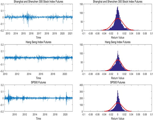
The empirical data used in this study are the daily return sequences of the main contracts of the Shanghai and Shenzhen 300 (CSI 300) stock index futures, Hang Seng stock index futures, and S&P 500 futures. The time span for the CSI 300 stock index futures is 2012/7/24–2021/4/23. The time span for the Hang Seng stock index futures is 2009/11/19–2021/4/23. The time span for the S&P500 futures is 2008/1/2–2021/4/23. The left column of Figure 1 shows the return sequence diagram of the three futures markets and the right column shows the return sequence distribution diagram for all three markets. We find that the extreme price fluctuations of the CSI 300 stock index futures are concentrated in the period from June to September 2015 and the beginning of 2020. The extreme price volatility of the S&P500 futures was concentrated from 2008 to 2009 and in the first half of 2020, and there were significant jumps. The right column of Figure 1 shows the distribution of the three futures markets’ return sequences, and we find that the return series all have the phenomenon of peaks and thick tails, and there are left-biased characteristics.

Figure 1. Campus environment detection system.

Source: Drawn by authors with the help of MATLAB software.

4.2. Margin VaR value

Under the three models, that is, GARCH-GPD, SVCJ-GPD and SE-SVCJ-GPD, we calculated the margin levels of the CSI 300, Hang Seng, and S&P 500 stock index futures under the default probabilities of 0.05, 0.025 and 0.01. The VaR values of the long and short positions for the futures of each stock index are listed in Table 1.

Table 1. Margin level estimation table for long and short positions.

CSI 300
	α = 0.05		α = 0.025		α = 0.01
	Model	Mean	moDel	Mean	Model	Mean
Long position	Garch-Gpd	−0.0208	Garch-Gpd	−0.0244	Garch-Gpd	−0.0319
	Svcj-Gpd	−0.0234	Svcj-Gpd	−0.0268	Svcj-Gpd	−0.0339
	SE-Svcj-Gpd	−0.0246	SE-Svcj-Gpd	−0.0258	SE-Svcj-Gpd	−0.0351
Short position	Garch-Gpd	0.0196	Garch-Gpd	0.0225	Garch-Gpd	0.0282
	Svcj-Gpd	0.0223	Svcj-Gpd	0.0251	Svcj-Gpd	0.0309
	SE-Svcj-Gpd	0.0238	SE-Svcj-Gpd	0.0281	SE-Svcj-Gpd	0.0338
Hang Seng
	α = 0.05		α = 0.025		α = 0.01
	Model	Mean	Model	Mean	Model	Mean
Long position	Garch-Gpd	−0.0171	Garch-Gpd	−0.0195	Garch-Gpd	−0.0243
	Svcj-Gpd	−0.0193	Svcj-Gpd	−0.0216	Svcj-Gpd	−0.0264
	SE-Svcj-Gpd	−0.0185	SE-Svcj-Gpd	−0.0220	SE-Svcj-Gpd	−0.0278
Short position	Garch-Gpd	0.0170	Garch-Gpd	0.0194	Garch-Gpd	0.0241
	Svcj-Gpd	0.0189	Svcj-Gpd	0.0213	Svcj-Gpd	0.0261
	SE-Svcj-Gpd	0.0182	SE-Svcj-Gpd	0.0218	SE-Svcj-Gpd	0.0266
SP 500
	α = 0.05		α = 0.025		α = 0.01
	Model	Mean	Model	Mean	Model	Mean
Long position	Garch-Gpd	−0.0142	Garch-Gpd	−0.0167	Garch-Gpd	−0.0178
	Svcj-Gpd	−0.0159	Svcj-Gpd	−0.0181	Svcj-Gpd	−0.0224
	SE-Svcj-Gpd	−0.0172	SE-Svcj-Gpd	−0.0215	SE-Svcj-Gpd	−0.0264
Short position	Garch-Gpd	0.0187	Garch-Gpd	0.0190	Garch-Gpd	0.0232
	Svcj-Gpd	0.0156	Svcj-Gpd	0.0178	Svcj-Gpd	0.0221
	SE-Svcj-Gpd	0.0195	SE-Svcj-Gpd	0.0197	SE-Svcj-Gpd	0.0245

Source: Calculated by authors via MATLAB software.

It can be seen from Table 1 that as the probability of default increases, the margin level increases significantly. This result remains consistent across the three futures markets. In general, the margin levels in the different futures markets are significantly different. It can be observed that the CSI 300 stock index futures market has the highest margin levels, followed by the Hang Seng Stock Index futures market, and the S&P 500 futures market is the smallest. We believe that one of the reasons for this is that the CSI 300 stock index futures market has a shorter establishment time than the Hang Seng and S&P 500 futures markets, the operation and supervision mechanisms are not mature enough, and the market is more likely to experience high volatility. By contrast, the VaR values obtained by the GARCH-GPD model are generally smaller than those of the SVCJ-GPD and SE-SVCJ-GPD models, which consider jumps. This indicates that the GARCH model has an insufficient market risk capture effect, and we can further consider jumps. In particular, self-exciting and clustering jumps can improve the ability to estimate market risk. It is worth noting that in the S&P 500 futures market, the margin level of the SVCJ-GPD model for short positions is lower than the GARCH-GPD model under the three default probabilities, but the SE-SVCJ-GPD model does not have such anomalies. The estimated results maintain stable consistency in different markets.

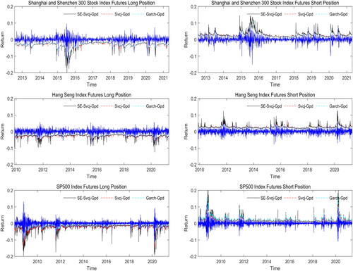
To better compare the empirical effects of each model; we take the default probability of 0.01 as an example. Figure 2 shows the predicted values of the long- and short-margin levels and the true returns of the three stock index futures markets. during periods of high volatility, the SE-SVCJ-GPD model captures more downside risks than the SVCJ-GPD and GARCH-GPD models for long positions, and the SE-SVCJ-GPD model captures more upper risks than the SVCJ-GPD and GARCH-GPD models for short positions. This shows that the SE-SVCJ-GPD model provides a more accurate prediction of the margin level than the SVCJ-GPD and GARCH-GPD models do. The main reason for this result is that jumps are an important source of risk in futures markets, and volatility under extreme events increases rapidly and becomes highly persistent. Its dynamics are not sufficiently characterized by Brownian motion alone. Therefore, the GARCH model has errors in estimating the risk above and below.

Figure 2. Real returns and VaR value of the three models.

Source: Drawn by authors with the help of MATLAB software.

4.3. Backtesting

To judge the predictive effect of the three types of models in this study, the failure frequency test method was used for backtesting (Kupiec, 1995). If the VaR of the dynamic margin for the long (short) positions is less than (greater than) the actual returns on the day, the prediction fails once. Table 2 shows the predicted and true values of the violation time and violation rate for the three markets under different default levels.

Table 2. Backtesting results: violation time and violation rate. Expect represents the true violation time at significance level α.

CSI 300	Long position		Short position
Model	Violation time	Violation rate	Violation time	Violation rate
Expect	107 (α = 0.05)
Garch-Gpd	113	0.0527	164	0.0765
Svcj-Gpd	91	0.0424	117	0.0546
SE-Svcj-Gpd	105	0.0490	110	0.0513
Model	Violation time	Violation rate	Violation time	Violation rate
Expect	53 (α = 0.025)
Garch-Gpd	81	0.0378	115	0.0536
Svcj-Gpd	65	0.0303	87	0.0406
SE-Svcj-Gpd	57	0.0266	57	0.0266
Model	Violation time	Violation rate	Violation time	Violation rate
Expect	21 (α = 0.01)
Garch-Gpd	35	0.0205	64	0.0298
Svcj-Gpd	29	0.0135	40	0.0186
SE-Svcj-Gpd	26	0.0121	34	0.0158
Hang Seng	Long position		short position
Model	Violation time	Violation rate	Violation time	Violation rate
Expect	144 (α = 0.05)
Garch-Gpd	205	0.0711	183	0.0634
Svcj-Gpd	208	0.0551	123	0.0433
SE-Svcj-Gpd	150	0.0519	128	0.0443
Model	Violation time	Violation rate	Violation time	Violation rate
Expect	72 (α = 0.025)
Garch-Gpd	149	0.0516	111	0.0384
Svcj-Gpd	116	0.0402	89	0.0308
SE-Svcj-Gpd	79	0.0273	63	0.0218
Model	Violation time	Violation rate	Violation time	Violation rate
Expect	29 (α = 0.01)
Garch-Gpd	74	0.0256	52	0.0180
Svcj-Gpd	63	0.0218	43	0.0149
SE-Svcj-Gpd	34	0.0117	22	0.0076
SP 500	Long position		short position
Model	Violation time	Violation rate	Violation time	Violation rate
Expect	174 (α = 0.05)
Garch-Gpd	292	0.0839	110	0.0316
Svcj-Gpd	233	0.0669	192	0.0551
SE-Svcj-Gpd	179	0.0514	183	0.0525
Model	Violation time	Violation rate	Violation time	Violation rate
Expect	87 (α = 0.025)
Garch-Gpd	209	0.0601	69	0.0198
Svcj-Gpd	167	0.0479	130	0.0373
SE-Svcj-Gpd	100	0.0287	90	0.0258
Model	Violation time	Violation rate	Violation time	Violation rate
Expect	35 (α = 0.01)
Garch-Gpd	175	0.0502	26	0.0075
Svcj-Gpd	107	0.0307	54	0.0155
SE-Svcj-Gpd	52	0.0149	30	0.0086

Source: Calculated by authors via MATLAB software.

In the three futures markets, the VaR and real returns are compared and analyzed in the three futures markets. The GARCH-GPD model roughly covers the volatility risk of a return sequence. However, when it is compared with SVCJ-GPD and SE-SVCJ-GPD models, the prediction effect of the GPD model is still not ideal, especially in the case of a short position, the GPD model has significant prediction errors. Under the 0.01 default level of the Hang Seng Stock Index futures market, the margin level obtained by the GARCH-GPD model is low, which results in a large number of days when the VaR value is less than the true return. This model cannot adequately cover volatility risk, which causes explosions. The possibility of warehouses has increased significantly. By contrast, the SVCJ-GPD and SE-SVCJ-GPD models, which consider jumps have a lower violation rate and are closer to the true default level. We believe that the main reason for this result is that, on the one hand, although the GARCH model can reflect the instantaneous fluctuation of prices in time, the volatility will increase rapidly and be highly persistent under extreme events. This type of volatility is difficult to capture through volatility diffusion norms, and its dynamics rely only on Brownian motion. On the other hand, the SVCJ model with a general jump process can be used to capture large changes in asset prices; once an extreme event occurs, the collapse of asset prices is not a single price jump. It has an obvious amplification and contagion effect, which makes jumps self-exciting and clustering under extreme events. Therefore, the SE-SVCJ model has a better ability to capture tail outliers and a better prediction effect than the SVCJ model.

5. Conclusion and discussion

5.1. Conclusion

This study combines extreme value theory with the SVCJ and SE-SVCJ models that characterize jumps to construct the SVCJ-GPD and SE-SVCJ-GPD models, which dynamically measure the optimal margin level for the index futures market and improve the forecast performance of VaR over the GARCH-GPD model. This hybrid method can appropriately model the leptokurtic fat-tailed distribution, asymmetry, leverage and clustering jumps of future returns and specifically capture extreme risk.

This study makes three major contributions to the literature: First, the VaR values obtained by the SVCJ-GPD and SE-SVCJ-GPD models are generally larger than the GARCH-GPD model (Chen & Yu, 2020). Jumps, especially self-exciting and clustering jumps, can improve the ability to estimate market risk and dynamically cover the risk of market price fluctuations.

Second, the SE-SVCJ-GPD model consistently provides optimal margin levels. In the S&P 500 futures market, the margin level based on the SVCJ-GPD model for short positions is lower than the GARCH-GPD model under the three default probabilities, but the SE-SVCJ-GPD model does not result in this type of anomaly.

Finally, during extreme events, the long (short) position based on the SE-SVCJ-GPD model captures more extreme lower (upper) risks than the SVCJ-GPD model, indicating that the SE-SVCJ-GPD model can provide more useful information and has the best dynamic margin setting ability.

5.2. Discussion

This study provides a better understanding of the futures markets. Financial regulators can establish a market-wide risk early warning mechanism to avoid risk spread, and risk managers can effectively assess risk levels and implement corresponding risk-prevention measures. However, this study has some limitations. We only verified the effectiveness of the method for the stock index, and the data used had some limitations. In the future, we can extend the application of this method to derivatives markets, commodity markets, and other fields. Second, this study proposes a hybrid method that integrates different models to obtain better results. In the next step, we can consider finding better statistics to improve prediction accuracy to adapt to complex financial environments.

Disclosure statement

No potential conflict of interest was reported by the authors.

Additional information

Funding

This work is partially supported by the MOE Layout Foundation of Humanities and Social Sciences (Grant No. 22YJA790007), the Science and Technology Innovation Program of Hunan Province (Grant No. 2021RC3057), and the Fundamental Research Funds for the Central Universities.

References

- Aït-Sahalia, Y. (2004). Disentangling diffusion from jumps. Journal of Financial Economics, 74(3), 487–528.
- Aït-Sahalia, Y., Cacho-Diaz, J., & Laeven, R. J. (2015). Modeling financial contagion using mutually exciting jump processes. Journal of Financial Economics, 117(3), 585–606. https://doi.org/10.1016/j.jfineco.2015.03.002
- Akgiray, V., & Booth, G. G. (1988). Mixed diffusion-jump process modeling of exchange rate movements. The Review of Economics and Statistics, 70(4), 631–637. https://doi.org/10.2307/1935826
- Angelidis, T., Benos, A., & Degiannakis, S. (2004). The use of Garch models in Var estimation. Statistical Methodology, 1(1-2), 105–128. https://doi.org/10.1016/j.stamet.2004.08.004
- Bates, D. S. (1996). Jumps and stochastic volatility: Exchange rate processes implicit in deutsche mark options. Review of Financial Studies, 9(1), 69–107. https://doi.org/10.1093/rfs/9.1.69
- Bates, D. S. (2019). How crashes develop: Intradaily volatility and crash evolution. The Journal of Finance, 74(1), 193–238. https://doi.org/10.1111/jofi.12732
- Bollerslev, T. (1986). Generalized autoregressive conditional heteroskedasticity. Journal of Econometrics, 31(3), 307–327. https://doi.org/10.1016/0304-4076(86)90063-1
- Booth, G. G., Broussard, J. P., Martikainen, T., & Puttonen, V. (1997). Prudent margin levels in the Finnish stock index futures market. Management Science, 43(8), 1177–1188. https://doi.org/10.1287/mnsc.43.8.1177
- Broussard, J. P. (2001). Extreme-value and margin setting with and without price limits. The Quarterly Review of Economics and Finance, 41(3), 365–385. https://doi.org/10.1016/S1062-9769(00)00083-1
- Carr, P., & Wu, L. (2017). Leverage effect, volatility feedback, and self-exciting market disruptions. Journal of Financial and Quantitative Analysis, 52(5), 2119–2156. https://doi.org/10.1017/S0022109017000564
- Chen, Y., & Yu, W. (2020). Setting the margins of Hang Seng index futures on different positions using an aparch-gpd model based on extreme value theory. Physica A: Statistical Mechanics and Its Applications, 544(123207), 123207. https://doi.org/10.1016/j.physa.2019.123207
- Cotter, J. (2001). Margin exceedences for European stock index futures using extreme value theory. Journal of Banking & Finance, 25(8), 1475–1502. https://doi.org/10.1016/S0378-4266(00)00137-0
- Duffie, D., & Pan, J. (2001). Analytical value-at-risk with jumps and credit risk. Finance and Stochastics, 5(2), 155–180. https://doi.org/10.1007/PL00013531
- Duffie, D., Pan, J., & Singleton, K. (2000). Transform analysis and asset pricing for affine jump-diffusions. Econometrica, 68(6), 1343–1376. https://doi.org/10.1111/1468-0262.00164
- Edwards, F. R., & Neftci, S. N. (1988). Extreme price movements and margin levels in futures markets. Journal of Futures Markets, 8(6), 639–655. https://doi.org/10.1002/fut.3990080602
- Engle, R. F. (1982). Autoregressive conditional heteroscedasticity with estimates of the variance of united kingdom inflation. Econometrica, 50(4), 987–1007. https://doi.org/10.2307/1912773
- Eraker, B., Johannes, M., & Polson, N. (2003). The impact of jumps in volatility and returns. The Journal of Finance, 58(3), 1269–1300. https://doi.org/10.1111/1540-6261.00566
- Figlewski, S. (1984). Margins and market integrity: Margin setting for stock index futures and options. Journal of Futures Markets, 4(3), 385–416. https://doi.org/10.1002/fut.3990040307
- Fulop, A., Li, J., & Yu, J. (2015). Self-exciting jumps, learning, and asset pricing implications. Review of Financial Studies, 28(3), 876–912. https://doi.org/10.1093/rfs/hhu078
- Gay, G. D., Hunter, W. C., & Kolb, R. W. (1986). A comparative analysis of futures contract margins. The Journal of Futures Markets (1986-1998), 6(2), 307.
- Goodell, J. W. (2020). COVID-19 and finance: Agendas for future research. Finance Research Letters, 35(101512), 101512.
- Hogenboom, F., Michael, d W., Frasincar, F., & Kaymak, U. (2015). A news event-driven approach for the historical value at risk method. Expert Systems with Applications, 42(10), 4667–4675. https://doi.org/10.1016/j.eswa.2015.02.002
- Hsieh, D. (1989). Testing for nonlinearity in daily foreign exchange rate changes. The Journal of Business, 62(3), 339–368. https://doi.org/10.1086/296466
- Iglesias, E. M. (2022). The influence of extreme events such as BREXIT and COVID-19 on equity markets. Journal of Policy Modeling, 44(2), 418–430. https://doi.org/10.1016/j.jpolmod.2021.10.005
- Junior, P. O., Tiwari, A. K., Tweneboah, G., & Asafo-Adjei, E. (2022). Gas and garch based value-at-risk modeling of precious metals. Resources Policy, 75, 102456.
- Kupiec, P. (1995). Techniques for verifying the accuracy of risk measurement models. The Journal of Derivatives, 3(2), 73–84.
- Longin, F. M. (1996). The asymptotic distribution of extreme stock market returns. The Journal of Business, 69(3), 383–408. https://doi.org/10.1086/209695
- Longin, F. M. (1999). Optimal margin level in futures markets: Extreme price movements. Journal of Futures Markets, 19(2), 127–152. https://doi.org/10.1002/(SICI)1096-9934(199904)19:2<127::AID-FUT1>3.0.CO;2-M
- Maciel, L. (2021). Cryptocurrencies value-at-risk and expected shortfall: Do regime-switching volatility models improve forecasting? International Journal of Finance & Economics, 26(3), 4840–4855. https://doi.org/10.1002/ijfe.2043
- Mansor, F., Al Rahahleh, N., & Bhatti, M. I. (2019). New evidence on fund performance in extreme events. International Journal of Managerial Finance, 15(4), 511–532. https://doi.org/10.1108/IJMF-07-2018-0220
- McNeil, A. J., & Frey, R. (2000). Estimation of tail-related risk measures for heteroscedastic financial time series: an extreme value approach. Journal of Empirical Finance, 7(3-4), 271–300. https://doi.org/10.1016/S0927-5398(00)00012-8
- Orhan, M., & Köksal, B. (2012). A comparison of garch models for var estimation. Expert Systems with Applications, 39(3), 3582–3592. https://doi.org/10.1016/j.eswa.2011.09.048
- Patra, S. (2021). Revisiting value-at-risk and expected shortfall in oil markets under structural breaks: The role of fat-tailed distributions. Energy Economics, 101, 105452. https://doi.org/10.1016/j.eneco.2021.105452
- Pickands, J. III, (1975). Statistical inference using extreme order statistics. The Annals of Statistics, 3, 119–131.
- Samuel, Y. M. Z-t. (2008). Value at risk and conditional extreme value theory via Markov regime switching models. Journal of Futures Markets, 28(2), 155–181. https://doi.org/10.1002/fut.20293
- Song, G., Xia, Z., Basheer, M. F., & Shah, S. M. A. (2021). Co-movement dynamics of us and Chinese stock market: Evidence from COVID-19 crisis. Economic Research-Ekonomska Istraživanja, 35(1), 2460–2476.
- Tucker, A. L., & Pond, L. (1988). The probability distribution of foreign exchanges: Tests of candidate processes. The Review of Economics and Statistics, 70(4), 638–647. https://doi.org/10.2307/1935827
- Venkateswaran, M., Wade, B. B., & Hall, J. A. (1993). The distribution of standardized futures price changes. Journal of Futures Markets, 13(3), 279–298. https://doi.org/10.1002/fut.3990130305
- Wang, L., Xu, Y., & Salem, S. (2021). Theoretical and experimental evidence on stock market volatilities: A two-phase flow model. Economic Research-Ekonomska Istraživanja, 34(1), 3245–3269. https://doi.org/10.1080/1331677X.2021.1874459
- Yao, Y., Cai, S., & Wang, H. (2022). Are technical indicators helpful to investors in china’s stock market? A study based on some distribution forecast models and their combinations. Economic Research-Ekonomska Istraživanja, 35(1), 2668–2692
- Yu, J. (2004). Empirical characteristic function estimation and its applications. Econometric Reviews, 23(2), 93–123. https://doi.org/10.1081/ETC-120039605
- Zhang, J. (2007). Likelihood moment estimation for the generalized pareto distribution. Australian & New Zealand Journal of Statistics, 49(1), 69–77. https://doi.org/10.1111/j.1467-842X.2006.00464.x