Government debt and household wealth inequality: evidence from China

Abstract

This study attempts to explain the relationship between government debt and household wealth inequality, and further discusses possible channels of influence to provide ideas for mitigating the increasing gap between rich and poor. This study puts forward relevant assumptions in the theoretical model, further analyses the composition of household wealth, and verifies that household housing investment is an essential factor. This study finds that the expansion of government debt raises the price of housing, leading to faster wealth growth for wealthy households with relatively more real estate and widening the gap between rich and poor. This study argues that in economic development, government debt should be tilted towards livelihood protection and infrastructure construction, providing guaranteed housing to eligible relatively poor and narrowing the gap between rich and poor to a reasonable extent.

Keywords:

• Government debt
• wealth distribution
• Gini coefficient
• land supply
• housing price

JEL CLASSIFICATIONS:

• D14
• H63
• H31

1. Introduction

In recent decades, income and wealth gaps in most countries have widened at different speeds. According to the World Inequality Report (Alvaredo et al., 2018) issued by the World Inequality Lab, the total income of the top 10% of China’s income accounted for 41% of the total national income in 2016; at the same time, from 1995 to 2015, the share of national wealth held by the wealthiest 1% increased from 15% to 30%.

A widening wealth gap is detrimental to economic growth and social stability (Liao & Zhang, 2021; Zhang et al., 2021). Fisher et al. (2020) studied the difference in the marginal propensity to consume in the distribution of wealth and found that low-wealth households cannot smooth consumption as much as other households do, implying that rising wealth inequality may reduce aggregate consumption, which in turn limits economic growth. Thorbecke and Charumilind (2002) explored the relationship between income inequality and social problems such as political instability, education, health and crime, and confirmed that income inequality is an important influencing factor. Therefore, where the gap between the rich and the poor widens, it is of great theoretical and practical importance to explore the issue of inequality.

As an essential component of fiscal policy, the impact of government debt on wealth distribution should be considered. According to data released by Ministry of Finance, the total debt of the Chinese government had reached 29.95 trillion Yuan by the end of 2017. These data exceeded one-third of the GDP of that year. While government debt covers the fiscal deficits and promotes economic development, the social welfare problems cannot be ignored. Existing studies have focused more on the impact of government debt on economic growth and implied financial risks (Arai et al., 2018; Dumitrescu et al., 2022; Fseifes & Warrad, 2020) and less on the distributional effects of government debt. Government debt is deferred taxation, reflecting certain distributional relationships. The existence of idle capital in society makes it possible for the government to issue debt, which means that the beneficiaries of government debt are the groups with idle capital in society, that is, the richer groups in society, and thus the phenomenon of the poor subsidising the rich (Salotti & Trecroci, 2018).

Because it is challenging to differentiate wealth among family members after an individual forms a family, some studies have measured wealth in terms of the household (e.g., the English Longitudinal Study of Ageing [Marshall et al., 2014]). In China’s current economic environment, how does government debt affect wealth distribution, and what are the channels through which its effects play out? Is there any variability across regions? As an extension of the study of the economic welfare of government debt, this study constructs a theoretical model based on existing studies and conducts an empirical analysis using China Household Finance Survey (hereafter abbreviated as CHFS).

The possible contributions of this study are as follows: First, by measuring the distribution of household wealth at the prefectural level in China, instead of choosing cross-country data, the interference of country-specific differences in the existing literature owing to political and economic systems or cultural practices on the empirical results is avoided. Second, by exploring the relationship between government debt and household wealth inequality, this study further reveals the impact of government debt from a micro perspective and also discusses the differences in the effect of government debt on household wealth inequality in regions with different economic development and different land structures. The findings of this study provide a targeted basis for the relevant departments to formulate government debt-related policies and provide ideas to achieve inclusive economic growth by weighing the efficiency and equity issues.

2. Literature review and theoretical models

2.1. Literature review

Wealth is a stock concept derived from income and wealth transfers in terms of the path of wealth accumulation. Income is transformed into wealth over time; thus, the long-term income inequality problem is likely to be transformed into a significant wealth inequality problem (Grabka, 2015). The initial wealth inequality caused by intergenerational transmission also influences the formation of new wealth inequality (Benton & Keister, 2017; Isaac, 2014; Klimaviciute et al., 2019).

From an income perspective, unequal distribution among factors is responsible for income disparities, with the rich holding a relatively larger share of capital income and the poor holding a relatively larger share of labour income, and a decline in the share of labour income, leading to a decline in wealth accumulation among the middle and lower classes (Wan & Zhou, 2005). Luo (2020) links rising inequality to a decline in labour share. Suppose the rate of return on capital is greater than that of economic growth. In that case, the share of capital rises, where ownership is concentrated in a minority group, and an increase in inequality is inevitable. The decline in labour share is mainly caused by external stochastic shocks, such as the structural transformation of the economy, capital-biased technological progress, and the development of financial markets (Zhang, 2017). Other studies analyse income inequality among workers based on heterogeneity. The shift in the mode of production is more substitutable for unskilled labour and less substitutable for skilled labour. Thus the change in market demand for labour raises the skill premium, exacerbating the income inequality among workers (Agranov & Palfrey, 2020; Ge & Yang, 2014; Shi, 2021).

From a wealth transfer perspective, wealth transfer inequality stems mainly from initial wealth inequality and inequality in the inheritance of labour endowments because of intergenerational transmission (Alan et al., 2015; Cagetti, 2003; Dynan et al., 2004). Compared with the poor, the rich prefer to save more, which allows them to accumulate more wealth. The rich give away more of their savings and inheritance to their children; thus, wealth inequality is rooted in savings behaviour and intergenerational linkages in wealth accumulation (Kotlikoff & Summers, 1981). Dynan et al. (2004) note that the combination of prevention and bequest motives stimulates savings in higher-income groups while having less impact on lower-income households. In addition, the redistribution system also amplifies the inequality of the primary distribution, and the rich group can enjoy more financial resources, tax incentives and financial subsidies from the government.

The impact of government debt on wealth inequality can also be analysed in terms of the two paths of wealth accumulation. Government debt affects the income distribution of both labour and capital. From the source of government debt funds, the funds required by the government are mainly financed through commercial banks and other financial institutions. By contrast, savings from idle funds finances the financial sector. The debt service of government debt can be indirectly passed on to individuals through financial institutions or directly through bond proceeds by issuing government bonds, raising the capital income of this group (Eltrudis & Monfardini, 2020; Galindo & Panizza, 2018). If the amount of government debt held is more progressive in the higher-income brackets than that of taxes paid, the government paying off debt with taxes leads to a flow of wealth from the lower-income brackets to the higher-income brackets (Salti, 2015). Mankiw (2000) has similar findings, where higher levels of debt imply the need to pass higher taxes to pay interest on the debt, and taxes affect both savers’ and spenders’ impact.

Nevertheless, savers bear interest payments entirely, whereas spenders already have lower income and consumption than savers; thus, higher debt levels increase income and consumption inequality. For the expenditure of government debt funds, the primary purpose of Chinese government debt issuance is to raise funds for national construction, most of which is used for national infrastructure construction. An increase in government debt investment in infrastructure construction increases the marginal rewards received by the capital factor in the development of various industries. However, the wage rewards of workers increase slowly (Huang et al., 2020).

Furthermore, increases in government debt also widen the gap in the initial inequality of wealth distribution. Michel and Pestieau (2005) argue that, although public debt is neutral in general, wealthy altruists with large capital stocks and public debt can increase their steady-state wealth by increasing their investment in public debt, causing a redistribution of wealth from poorer non-altruists to more affluent. Borissov and Kalk (2020) construct an endogenous growth model, arguing that the critical mechanism by which long-run wealth inequality arises relies on factors related to social status. Consumers’ consideration of consumption levels depends not only on absolute consumption levels but also on social status. In a two-tier system, eventually, the rich own all the capital and public debt in society, and all other poor people become poorer. Furthermore, government policies aimed at reducing inequality by increasing public debt can increase inequality in the long run when the initial wealth is unequally distributed in a given environment.

2.2. Theoretical model

The theoretical model builds on the framework constructed by Bräuninger (2005), which analyzes the impact of public debt on economic growth. The model in this study is extended: the original homogeneous group is divided into two groups, the rich and the poor, and indicators measuring wealth inequality are introduced while calculating wealth accumulation, which in turn allows the impact of government debt on wealth inequality to be analysed in the dynamic model; at the same time, considering that household wealth is accumulated from both income and wealth transfer channels, the factor of inherited bequests is added to the utility function of the household sector.

2.2.1. Family sector

In this study, each individual’s life cycle contains two periods, and individuals born in the period $t$ are noted as $t$ generation. Thus, there are two generations in the period $t:$ generation $t$ (younger generation) and generation $t-1$ (older generation). The household sector is divided into the poor and the rich, denoted as $P$ and $R.$ Suppose that the share of the rich in the household sector is $\theta$ (among others $\theta \in (0,1)$). In each period, the number of newborns is $N_t.$ Each individual provides undifferentiated labour for labour remuneration in the younger period, and the total labour supply is the same as the number of newborns. The older period will withdraw from the labour market, rely on the wealth accumulated in the younger period, and gift part of it to future generations.

The maximum utility of each individual born in the period $t$ is: (1) $$U_t^i=(1-{\alpha }_i)\hspace{0.17em}\log \hspace{0.17em}{c}_t^{1i}+{\alpha }_i[(1-\beta )\hspace{0.17em}\log \hspace{0.17em}{c}_{t+1}^{2i}+\beta \hspace{0.17em}\log \hspace{0.17em}{b}_{t+1}^i]$$(1) where $c_t^{1i}$ is consumption in the younger period, $c_{t+1}^{2i}$ is consumption in the older period, and $b_{t+1}^i$ is wealth gifted to future generations. ${\alpha }_i$ is the intertemporal preference parameter (${\alpha }_i\in (0,1)$), and $\beta$ is the gifting preference parameter ($\beta \in (0,1)$). Referring to the settings and empirical data in the existing literature, the rich will choose to save more income compared to the poor, and thus the intertemporal preference parameter is larger for the rich than for the poor, i.e., ${\alpha }_R>{\alpha }_P$ (Becker, 1980; Dynan et al., 2004). The gifting preference parameter does not differ between the rich and the poor (Bossmann et al., 2007). In addition, this study assumes that the initial wealth endowment of the older generation is greater for the rich than for the poor. The following relationship is satisfied for the consumption levels of the two phases of the $t$ generations. （2a） $$c_t^{1i}=(1-{\tau }_t)w_t-s_t^i+b_t^i$$（2a） （2b） $$c_{t+1}^{2i}=[1+(1-{\tau }_{t+1})r_{t+1}]s_t^i-b_{t+1}^i$$（2b） where $s_t^i$ is savings in the young period, $w_t$ is the wage rate, ${\tau }_t$ is the tax rate, and $r_{t+1}$ is the return on capital (risk-adjusted). The savings are obtained to satisfy the following relationship. (3) $$s_t^i={\alpha }_i[(1-{\tau }_t)w_t+\beta (1+(1-{\tau }_t)r_t)s_{t-1}^i]$$(3)

Total social savings $M_t$ (total wealth) in period $t$ are: (4) $$M_t=\theta s_t^R{N}_t+(1-\theta )s_t^P{N}_t$$(4)

Combining Equations (3)(3) $$s_t^i={\alpha }_i[(1-{\tau }_t)w_t+\beta (1+(1-{\tau }_t)r_t)s_{t-1}^i]$$(3) and (4)(4) $$M_t=\theta s_t^R{N}_t+(1-\theta )s_t^P{N}_t$$(4) yields: (5) $$M_t=\overline{\alpha }(1-{\tau }_t)w_t{N}_t+\beta [1+(1-{\tau }_t)r_t][{\alpha }_R{s}_{t-1}^R\theta N_t+{\alpha }_P{s}_{t-1}^P(1-\theta )N_t]$$(5) where $\overline{\alpha }=\theta {\alpha }_R+(1-\theta ){\alpha }_P.$ Let the ratio of the wealth held by the rich to the total wealth of society be ${\sigma }_t.$ This ratio measures the degree of inequality, i.e., ${\sigma }_t=\theta s_t^R{N}_t/M_t.$

2.2.2. Corporate sector

Assume that the firm sectors produce a single final good through technology, capital, and labour, and that their production functions obey the Cobb-Douglas form. (6) $$Y_t=A{K}_t^{\gamma }{(a_t{N}_t)}^{1-\gamma }(0<\gamma <1)$$(6) where $a_t$ is labour productivity. This study assumes that the average capital per worker has a positive external influence on labour productivity, which depends on the accumulation of knowledge through ‘learning by doing’ and the existence of $a_t=K_t/N_t.$ The household sector invests in two broad assets: physical capital and government bonds, which pay the same rate of return on capital $r_t.$ The capital and labour markets are perfectly competitive, and the supply of capital and labour is exogenous in each period. As a result of market competition, the rate of return on capital and the wage rate adjust to equalise the supply and demand of capital and labour when the interest rate corresponds to the marginal product of capital and the wage rate corresponds to the marginal product of labour. The wage rate and the rate of return on capital satisfy the following equations. （7a） $$w_t=A(1-\gamma )K_t/N_t$$（7a） （7b） $$r_t=A\gamma$$（7b）

2.2.3. Government sector

Government departments obtain funds for government spending through collection taxes and bond issuance, and the government budget constraint satisfies the following equation. (8) $$D_{t+1}-D_t+T_t=G_t+r_t{D}_t$$(8) where government spending is $G_t.$ According to the existing literature (Bräuninger, 2005), this study assumes a fixed ratio $g$ ($g\in (0,1)$) between government spending and GDP. Let the government debt ratio be $d$ and the government tax revenue be $T_t.$ Although most of the household assets are deposited in pension accounts for some Western countries, capital income cannot be ignored in the case of China. At the same time, China has not yet levied relevant taxes on inheritance income. Hence, the taxation sources are wage and capital income, and the relationship between the variables is satisfied. （9a） $$G_t=g{Y}_t$$（9a） （9b） $$D_{t+1}-D_t=d{Y}_t$$（9b） （9c） $$T={\tau }_t(w_t{N}_t+r_t{M}_{t-1})$$（9c）

Let the ratio of government debt to private investment be $x_t,$ i.e. $x_t=D_t/K_t.$ Combining Equations (6)(6) $$Y_t=A{K}_t^{\gamma }{(a_t{N}_t)}^{1-\gamma }(0<\gamma <1)$$(6) , (7b)（7b） $$r_t=A\gamma$$（7b） , (8)(8) $$D_{t+1}-D_t+T_t=G_t+r_t{D}_t$$(8) , (9a)（9a） $$G_t=g{Y}_t$$（9a） , (9b)（9b） $$D_{t+1}-D_t=d{Y}_t$$（9b） and (9c)（9c） $$T={\tau }_t(w_t{N}_t+r_t{M}_{t-1})$$（9c） , the tax rate ${\tau }_t$ is: (10) $${\tau }_t=1-(1+d-g)/(1+\gamma x_t)$$(10)

2.2.4. Market equilibrium analysis

The purpose is to compare the equilibrium levels of wealth inequality at steady states with different government debt rates. The resource constraints that are satisfied at market equilibrium are: (11) $$Y_t=(\theta (c_t^{1R}+c_t^{2R})N_t+(1-\theta )(c_t^{1P}+c_t^{2P})N_t)+(K_{t+1}-K_t)+G_t$$(11)

The market clearing condition is $M_t=K_{t+1}+D_{t+1},$ by substituting $x_t,$ the following relationship is obtained. (12) $$K_t=M_{t-1}/(1+x_t)$$(12)

The above conditions allow for analysing the equilibrium path of the variables in the economy.

First, measure the growth rate of total social savings, calculate $M_t/M_{t-1},$ and substitute Equations (7a)（7a） $$w_t=A(1-\gamma )K_t/N_t$$（7a） , (7b)（7b） $$r_t=A\gamma$$（7b） , (10)(10) $${\tau }_t=1-(1+d-g)/(1+\gamma x_t)$$(10) and (12)(12) $$K_t=M_{t-1}/(1+x_t)$$(12) into Equation (5)(5) $$M_t=\overline{\alpha }(1-{\tau }_t)w_t{N}_t+\beta [1+(1-{\tau }_t)r_t][{\alpha }_R{s}_{t-1}^R\theta N_t+{\alpha }_P{s}_{t-1}^P(1-\theta )N_t]$$(5) to obtain the following relationship. （13a） $$G^M(x_t,{\sigma }_{t-1})=\frac{M_t}{M_{t-1}}=\frac{\overline{\alpha }(1-\gamma )\mu }{(1+x_t)(1+\gamma x_t)}+\beta (1+\frac{\gamma \mu }{1+\gamma x_t})[({\alpha }_R-{\alpha }_P){\sigma }_{t-1}+{\alpha }_P]$$（13a） where $\mu =A(1+d-g).$

Next, the growth rate of government debt $D_{t+1}/D_t$ is calculated, and by associating Equations (6)(6) $$Y_t=A{K}_t^{\gamma }{(a_t{N}_t)}^{1-\gamma }(0<\gamma <1)$$(6) and (9b), the following relationship is obtained. （13b） $$G^D(x_t)=D_{t+1}/D_t=1+dA/x_t$$（13b）

Finally, the growth rate of private investment, calculated $K_{t+1}/K_t,$ by associating Equations (12)(12) $$K_t=M_{t-1}/(1+x_t)$$(12) and (9b), yields the following relationship. （13c） $$\begin{array}{c}{G}^K(x_t,{\sigma }_{t-1})=\mathrm{ }\mathrm{ }{K}_{t+1}/K_t=M_t/K_t-(d{Y}_t+D_t)/K_t\mathrm{ }\\ =\mathrm{ }\mathrm{ }(1+x_t)G^M(x_t,{\sigma }_{t-1})-(x_t+dA)\end{array}$$（13c）

According to Bräuninger (2005), capital and public debt growth depend on the deficit and the debt-to-capital ratios. If the debt-to-capital ratio remains constant, capital and public debt growth rates remain constant. In the steady state, public debt and capital grow at the same rate. Thus when the economy is in a steady state, i.e., $x_t=x_{t-1},$ the growth rate of government debt remains the same as the growth rate of private investment. Combining Equations (13b) and (13c) and substituting (13a) yields the following relationship. (14) $${\sigma }_{t-1}=\frac{(1+\gamma x_t)(1+x_t)(1+dA/x_t)-\overline{\alpha }(1-\gamma )\mu }{\beta (1+x_t)[1+\gamma (x_t+\mu )]({\alpha }_R-{\alpha }_P)}-\frac{{\alpha }_P}{{\alpha }_R-{\alpha }_P}$$(14)

Derivation of ${\sigma }_{t-1}$ from Equation (14)(14) $${\sigma }_{t-1}=\frac{(1+\gamma x_t)(1+x_t)(1+dA/x_t)-\overline{\alpha }(1-\gamma )\mu }{\beta (1+x_t)[1+\gamma (x_t+\mu )]({\alpha }_R-{\alpha }_P)}-\frac{{\alpha }_P}{{\alpha }_R-{\alpha }_P}$$(14) yields the relationship between the government debt ratio $d$ and the ratio ${\sigma }_{t-1}$ of wealth owned by the rich to the total wealth of society. (15) $$\frac{\mathrm{d}{\sigma }_{t-1}}{\mathrm{d}d}=\frac{A(1+\gamma x_t)[(1+x_t^{-1})(1+\gamma \mu -\gamma dA)-(1-\gamma )\overline{\alpha }]}{({\alpha }_R-{\alpha }_P)\beta (1+x_t){[1+\gamma (x_t+\mu )]}^2}$$(15) where $1+x_t^{-1}>1,$ $1+\gamma \mu -\gamma dA=1+\gamma A(1-g)>1,$ $0<(1-\gamma )\overline{\alpha }<1,$ ${\alpha }_R>{\alpha }_P,$ therefore $\mathrm{d}{\sigma }_{t-1}/\mathrm{d}d>0.$

This result reflects a positive relationship between the government debt ratio and wealth inequality; that is, increasing government debt promotes wealth inequality. Therefore, this study proposes the hypothesis:

H1: Higher government debt rates will lead to increased wealth inequality.

3. Data description and statistical analysis

3.1. Data source

The data used in this study to measure household wealth comes from CHFS. In 2013, 2015 and 2017, a total of 29 provinces (excluding Tibet and Xinjiang) in China were surveyed, and in 2011, 25 provinces (excluding Tibet, Xinjiang, Inner Mongolia, Fujian, Hainan and Ningxia) in China were surveyed.

3.2. Variable description

3.2.1. Dependent variable: household wealth inequality

Since it is challenging to differentiate wealth among family members after respondents form a household, household wealth is measured by household’s net worth on a household basis. There are many proxy variables to measure inequality in the existing literature. This study selects two indicators to measure wealth inequality, the top 20% household wealth share and the wealth Gini Coefficient. The sample was quintile-scored by year by year in a prefecture-level city. After conducting quintiles, the sample size of each group accounted for approximately 20%.

3.2.2. Independent variable: government debt ratio

The government debt ratio is the ratio of government debt to GDP. Referring to existing measures of government debt in China, government debt arises mainly from the imbalance between government revenues and expenditures. The external funds the government needs can be based on the investment expenditure on municipal infrastructure construction minus the available revenue. The obtainable revenue includes three components: budgetary funds, funds from land concessions for investment, and the funds obtained from the cash income of investment projects. Government debt includes two components, the sum of the government bond balance and the municipal bond balance.

3.2.3. Control variables and mechanism variables

Mechanism variables explore how government debt affects household wealth inequality. This study also controls for individual and year-fixed effects to control for the effects of factors associated with individuals that do not vary over time and the effects of macroeconomic factors associated with a particular year.

Table 1 provides details of the variables. Table 2 reports the results of descriptive statistics for the sample data. This study subjected all continuous variables to a 1% tail reduction.

Table 1. The symbol and definition of the variables.

Variable	Variable symbol	Definition
Dependent variable
Top 20% household wealth share (Ratio)	Wealth_top20	The ratio of the highest group to the overall wealth
Wealth Gini Coefficient (Ratio)	Wealth_gini	The difference between the ratio of the highest group and the lowest group to the overall wealth
Independent variable
Government Debt Ratio (Ratio)	Gebt_gdp	The ratio of government debt to GDP
Control variable
Economic Development Level	Ingdp	The natural logarithm of GDP
Financial development Level (Ratio)	Finance_gdp	The ratio of deposits and loans to GDP
Unemployment rate (Ratio)	Unemploy_rate	The ratio of unemployed labor force to total labour force
Fiscal deficit ratio (Ratio)	Deficit_gdp	The ratio of deficit to GDP
Mechanism variable
Bank loan (log)	Loan	Bank loans obtained by households
Household wealth (log)	Wealth	Total household wealth
Real Estate (Dummy)	Real Estate	Whether the household own house
Purchase Demand (Dummy)	Purchase Demand	Whether the household has the desire to purchase a house
Share of Real Estate (Ratio)	House Share	The ratio of house value to total wealth
Edu	Edu	Years of education (Head of household)
Age	Age	Age (Head of household)
Marriage (Dummy)	Marriage	Married or not (Head of household)
Health (Dummy)	Health	Health Level (Head of household)

Source: Authors Calculation.

Table 2. Data statistics.

Variable	Mean	Std.	25% quantile	Median	75% quantile
Wealth_top20	0.626	0.083	0.574	0.622	0.680
Wealth_gini	0.619	0.091	0.564	0.613	0.678
Gebt_gdp	0.087	0.049	0.052	0.079	0.110
Ingdp	9.899	0.783	9.477	9.945	10.359
Finance_gdp	0.032	0.031	0.018	0.026	0.035
Unemploy_rate	3.373	0.575	3.100	3.400	3.700
Deficit_gdp	0.111	0.102	0.049	0.075	0.123

Source: Authors Calculation.

3.3. Statistical analysis

The 2017 CHFS survey data shows that the average household wealth is about $1,247,800. Table 3 shows the household wealth breakdown of the 2017 CHFS survey. The household sample contains both rural and urban samples. Among the wealth held by households, real estate accounts for about 74.10% of the total wealth, which is the main component of household wealth.

Table 3. Household sub-wealth status (Unit: million yuan).

	10%	25%	50%	75%	90%	Mean
Production and operation	0.05	0.14	0.58	4.00	20.15	15.52
Real estate	0.00	3.01	26.04	87.08	240.00	92.46
Vehicles	1.00	3.00	7.00	13.50	24.00	10.78
Financial assets	0.05	0.21	1.30	7.00	24.00	9.18
Other assets	0.05	0.27	1.00	2.00	5.00	1.89
(Other liabilities)	(0.27)	(0.80)	(2.00)	(5.00)	(11.00)	(5.05)

Source: Authors Calculation.

4. Empirical analysis

4.1. Benchmark regression

To explore the effect of government debt on household wealth inequality, the study constructs a benchmark regression model as shown in Equation (16)(16) $$\mathit{Wealth}\_\mathit{unequalit}{y}_{it}={\alpha }_0+{\alpha }_{1}D\mathit{ebt}\_gd{p}_{it}+Z_{it}^{\prime }\alpha +D_i+D_t+{\epsilon }_{it}$$(16) . (16) $$\mathit{Wealth}\_\mathit{unequalit}{y}_{it}={\alpha }_0+{\alpha }_{1}D\mathit{ebt}\_gd{p}_{it}+Z_{it}^{\prime }\alpha +D_i+D_t+{\epsilon }_{it}$$(16)

The dependent variables are household wealth inequality, measured by the top 20% household wealth share ($\mathit{Wealth}\_\mathit{top}{20}_{it}$) and wealth Gini coefficient ($\mathit{Wealth}\_\mathit{gin}{i}_{it}$). The core explanatory variable is the government debt rate ($\mathit{Gebt}\_gd{p}_{it}$). The vector group of control variables $Z_{it}^{\prime }$ covers economic development status ($\mathit{Ingd}{p}_{it}$ and $\mathit{Ingdp}{2}_{it}$), unemployment rate ($\mathit{Unemploy}\_\mathit{rat}{e}_{it}$), level of financial development ($\mathit{Finance}\_gd{p}_{it}$) and fiscal deficit rate ($\mathit{Deficit}\_gd{p}_{it}$). Both individual fixed effects ($D_i$) and year fixed effects ($D_t$) are introduced into the regression equation.

In terms of model selection, considering the characteristics of the panel structure of ‘big N and small T’, both fixed-effects and random-effects models are used for regression to ensure the consistency of the estimation result. The data used in this study have some time series correlation, so columns (3) and (7) are corrected for clustering robust standard errors according to regions. Since the data used in this study are small samples, columns (4) and (8) are further considered in the small sample case using the Jackknife method. The results in Table 4 show that the estimated coefficients of government debt on household wealth inequality are significantly positive in all regressions.

Table 4. Relationship between government debt and household wealth inequality.

Variable	Wealth_top20				Wealth_gini
	FE	FE	RE +  Clustering	RE +  Jackknife	FE	FE	RE +  Clustering	RE +  Jackknife
	(1)	(2)	(3)	(4)	(5)	(6)	(7)	(8)
Gebt_gdp	0.282** (0.127)	0.305** (0.134)	0.429*** (0.117)	0.429*** (0.103)	0.322** (0.137)	0.350** (0.141)	0.490*** (0.126)	0.490*** (0.110)
Ingdp		−0.181 (0.233)	0.034 (0.109)	0.034 (0.103)		−0.276 (0.247)	0.026 (0.124)	0.026 (0.120)
Ingdp2		0.008 (0.012)	−0.002 (0.005)	−0.002 (0.005)		0.014 (0.012)	−0.002 (0.006)	−0.002 (0.006)
Unemploy_rate		−0.021 (0.017)	−0.002 (0.009)	−0.002 (0.009)		−0.023 (0.018)	−0.003 (0.010)	−0.003 (0.009)
Finance_gdp		−0.107 (0.098)	−0.117 (0.120)	−0.117 (0.105)		−0.126 (0.107)	−0.149 (0.129)	−0.149 (0.115)
Deficit_gdp		−0.096 (0.083)	−0.043 (0.081)	−0.043 (0.067)		−0.116 (0.090)	0.055 (0.084)	0.055 (0.073)
Individual fixed effect	Yes	Yes	Yes	Yes	Yes	Yes	Yes	Yes
Year fixed effect	Yes	Yes	Yes	Yes	Yes	Yes	Yes	Yes
Sample size	574	574	574	574	574	574	574	574
R-squared	0.175	0.121	0.190	0.190	0.181	0.091	0.197	0.197

Source: Authors Calculation.

The impact of government debt on each subgroup is reported in Table 5. The estimated coefficients of government debt on the wealth share of the top 20% and the next highest 20% of households are positive. In comparison, the estimated coefficients of the other three groups are negative. This result supports the conclusion that the effect is achieved by increasing the relatively rich households’ wealth share and decreasing the relatively poor households’.

Table 5. Results of subgroup test.

Variable	Minimum 20%	Next lower 20%	Middle 20%	Next higher 20%	Maximum20%
	(1)	(2)	(3)	(4)	(5)
Gebt_gdp	−0.126*** (0.034)	−0.076** (0.039)	−0.079* (0.047)	0.029 (0.122)	0.305** (0.134)
Ingdp	−0.081 (0.055)	0.007 (0.068)	0.053 (0.085)	0.096 (0.182)	−0.181 (0.233)
Ingdp2	0.006* (0.003)	0.000 (0.003)	−0.002 (0.004)	−0.004 (0.009)	0.008 (0.012)
Unemploy_rate	0.005*** (0.002)	0.004 (0.004)	0.003 (0.005)	−0.002 (0.007)	−0.021 (0.017)
Finance_gdp	0.023 (0.020)	0.010 (0.023)	0.034 (0.035)	−0.024 (0.055)	−0.107 (0.098)
Deficit_gdp	0.026* (0.015)	0.017 (0.021)	0.043 (0.028)	0.060 (0.054)	−0.096 (0.083)
Individual fixed effect	Yes	Yes	Yes	Yes	Yes
Year fixed effect	Yes	Yes	Yes	Yes	Yes
Sample size	574	574	574	574	574
R-squared	0.160	0.128	0.092	0.010	0.121

Source: Authors Calculation.

Further examination of the survey data shows that property land accounts for about 74.10% of total household wealth and is the main wealth held by households, especially in the top 20% of households where real estate accounts for about 83.12% of total wealth comprising the real estate of the bottom 20% which accounts for about 32.48%. The existing literature confirms the role of government debt in driving house prices, and government debt revenue is an essential component of broad-based land finance, which positively drives local house prices (Cai et al., 2021; Hu et al., 2021). The capital-attracting effect of government debt leads to an over-allocation of land resources to the industrial sector and, therefore, a shortage of commercial land resources, leading to a rapid increase in house prices (Akai & Sato, 2011; Cai & Treisman, 2005). The increase in government debt promotes the appreciation of property land, and relatively wealthy households own more property, so the wealth of relatively wealthy households grows faster, which widens household wealth inequality.

4.2. Robustness test

4.2.1. Change the proxy variables

The proxy variable of household wealth inequality is changed, and the calibre of its measurement is changed from prefecture-level city to province-based. Change the proxy variable for government debt, using the sum of government bond balance and municipal investment debt to GDP (Gebt_gdp2). The results in Table 6 show that government debt still has a significant positive effect on household wealth inequality after changing the proxy variables.

Table 6. Results of robustness test.

Variable	Wealth_top20		Wealth_gini
	Province	City	Province	City
	(1)	(2)	(3)	(4)
Gebt_gdp	0.387** (0.181)		0.662** (0.293)
Gebt_gdp2		0.391** (0.189)		0.431** (0.248)
Controls	Yes	Yes	Yes	Yes
Individual fixed effect	Yes	Yes	Yes	Yes
Year fixed effect	Yes	Yes	Yes	Yes
Sample size	112	574	112	574
R-squared	0.191	0.050	0.133	0.013

Note: Other control variables (Controls) are the same as in Table 4 and are not reported due to space limitations (Same below).

Source: Authors Calculation.

4.2.2. Deal with the endogeneity problem

Table 7 uses systematic GMM regression analysis to mitigate the endogeneity problem due to reverse causality, omitted variables, and other issues.

Table 7. Results of endogeneity problem.

Variable	Wealth_top20		Wealth_gini
	City	Province	City	Province
	(1)	(2)	(3)	(4)
Gebt_gdp	0.498*** (0.188)	0.459*** (0.179)	0.550** (0.221)	0.539*** (0.200)
Controls	Yes	Yes	Yes	Yes
Individual fixed effect	Yes	Yes	Yes	Yes
Year fixed effect	Yes	Yes	Yes	Yes
Sample size	574	112	574	112
AR (1)	0.032	0.007	0.092	0.057
AR (2)	0.230	0.956	0.232	0.164
Hansen	0.199	0.681	0.669	0.577

Note: AR (1), AR (2) and Hansen in the GMM regressions report the p-values of the GMM first-order and second-order serial correlation tests and the Hansen test.

Source: Authors Calculation.

4.3. Mechanism analysis

According to existing studies, local governments’ monopoly on agricultural land acquisition and land use is the basis of land finance (Liu et al., 2022; Wang et al., 2021). Many local governments have established urban construction investment companies as government financing platforms. So the governments have raised large-scale debt with land as collateral and land concession proceeds as the source of repayment (Cheng et al., 2022).

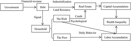
From the point of view of the household sector, the government’s issuance of debt undoubtedly releases the signal that house prices will rise in the future, attracting the household sector to invest in real estate. Regarding psychological factors, the rich are more willing to invest capital relative to their sources (Chiodi et al., 2012). In terms of external resources, the rich are more likely to use their existing property as security to obtain bank credit resources (Sakuragawa et al., 2021). Thus, the rich accumulate household wealth by purchasing a house through bank loans. In addition, families with a house can pass it on intergenerationally and inherit it from the next generation. The poor can only accumulate wealth through their daily wages. Rising house prices lead to a higher value of the house, and thus the rich accumulate wealth faster, leading to greater wealth inequality.

Figure 1 depicts this impact pathway, and the next part of the study focuses on the household sector to verify this impact pathway. Also, this study further validates this pathway by classifying regions through property purchase restriction policies and industrial land size.

Figure 1. Analysis of impact mechanism.

Source: The authors.

4.3.1. Micro-level mechanism analysis

The following analysis of its impact mechanism complements the micro-level empirical evidence. For this purpose, this study uses data from the CHFS survey for 2015 and 2017; mainly through the channel that government debt affects household capital investment and thus amplifies pre-existing wealth inequality. According to the previous analysis of household wealth composition, housing is an important component of household wealth, and the impact of housing price fluctuations on households’ financial participation and asset portfolios cannot be ignored (Waxman et al., 2020; Zhang, 2019).

First, this study analyses whether the level of household wealth affects the size of credit they obtain when purchasing a house. Since financial resources are scarce, households with specific wealth accumulation can enjoy more financial resources. The size of the credit acquired to purchase a house is used as a proxy variable through the logarithm of the commercial bank loan, and the independent variable is household wealth. This study controls factors related to human capital, including the age of the household head and its squared term, years of education, marital status, and health status. Column (1) in Table 8 reports the relationship between household wealth and the size of the credit. The results indicate that the greater the household’s initial wealth, the greater the size of the credit. The relationship between government debt and household wealth is further analysed. The results are shown in column (2) of Table 8, where an increase in government debt raises the initial wealth of households. The results indicate that an increase in government debt increases the household’s wealth, which helps the household obtain more home purchase loans.

Table 8. Results of microscopic mechanism test.

Variable	Loan	Wealth	Real Estate	Purchase Demand	House share
	(1)	(2)	(3)	(4)	(5)
Panel A: OLS
Wealth	0.035*** (0.002)
Debt_gdp		3.236*** (0.220)	0.183*** (0.023)	0.269*** (0.023)	0.059** (0.024)
Edu	0.008*** (0.001)	0.100*** (0.001)	0.002*** (0.000)	0.002*** (0.000)	0.004*** (0.000)
Age	−0.016*** (0.001)	0.020*** (0.002)	0.015*** (0.001)	−0.008*** (0.001)	0.013*** (0.001)
Age2	0.011*** (0.001)	−0.014*** (0.002)	−0.014*** (0.001)	0.004** (0.001)	−0.011*** (0.001)
Marriage	0.022*** (0.005)	0.238*** (0.013)	0.105*** (0.004)	0.006* (0.003)	0.065*** (0.004)
Health	0.015*** (0.004)	0.266*** (0.009)	0.015*** (0.002)	0.017*** (0.003)	0.004 (0.003)
Sample size	77 056	77 056	77 056	77 056	77 056
R-squared	0.039	0.246	0.030	0.041	0.017
Panel B: 2SLS
Wealth	0.298*** (0.013)
Debt_gdp		1.739*** (0.548)	0.273*** (0.046)	0.128*** (0.045)	0.130*** (0.048)
Controls	Yes	Yes	Yes	Yes	Yes
Sample size	77,056	77,056	77,056	77,056	77,056
R-squared	0.272	0.246	0.030	0.041	0.017

Note: Control variables in Panel B are the same as those in Panel A.

Source: Authors Calculation.

On this basis, the impact of government debt on household capital investment is examined. Households with access to more financial resources are more likely to make capital investments, especially in real estate. Columns (3) and (4) of Table 8 report the effect of government debt on whether a household owns the house and whether it intends to purchase a house in the future, respectively. The results show that households with a house and those purchasing a house increase under the influence of high government debt. Thus, soaring government debt promotes household investment in real estate.

Meanwhile, column (5) of Table 8 analyses the effect of government debt on the value of a house as a share of total household wealth, and the results show that as government debt increases, the ratio of the house also increases. Since different households own different shares of houses, they are affected by government debt differently. Relatively wealthy households own more houses, and their wealth grow faster, and government debt contributes to household wealth growth while increasing household wealth inequality.

To further eliminate the effect of the endogeneity problem, this study uses the instrumental variables. The instrumental variable chosen for household initial wealth is the initial wealth of other households in this prefecture-level city. Because household wealth is influenced not only by its economic factors but also by the status of local economic and social development. At the same time, the wealth level of other households can only influence the size of the loan obtained by this household when purchasing a house through the wealth level of this household. The instrumental variable chosen for government debt is lagged one-period land concession revenue. The government can quickly obtain construction funds by using land concession revenue as a guarantee, and there is a strong correlation between land concession revenue and government debt. The government’s land concession revenue does not directly affect household wealth but indirectly through economic growth, house prices, and land prices. The regression results of two-stage least squares are reported in Panel B of Table 8, which are consistent with the estimation results in each part of Panel A.

4.3.2. Heterogeneity analysis

This section classifies the sample into eastern and other regions to analyse whether the effect of government debt on household wealth inequality differs across different economic development levels. The results are shown in columns 1 and 2 of Table 9. In other regions, as government debt increases, household wealth inequality also increases, but the relationship between the two is not significant in the eastern region. This is because Beijing took the lead in introducing purchase restrictions in 2010, and the 24 cities that introduced purchase restrictions between 2010 and 2011 are mainly located in the eastern region, which has a more comprehensive housing management policy than other regions. The introduction of housing policies has led to the return of the role of housing from capital investment to residential use. It has been effective to a certain extent, so the impact of government debt on household wealth inequality in the eastern region is not significant.

Table 9. Results of heterogeneity test.

Variable	Economic development level		Industrial land
	Eastern	Other	More	Less
	(1)	(2)	(3)	(4)
Debt_gdp	0.127 (0.308)	0.378** (0.174)	0.367** (0.150)	0.227 (0.352)
Controls	Yes	Yes	Yes	Yes
Individual fixed effect	Yes	Yes	Yes	Yes
Year fixed effect	Yes	Yes	Yes	Yes
Sample size	178	396	306	268
R-squared	0.254	0.200	0.220	0.202

Note: The proxy variable for household wealth inequality is the ratio of wealth of the top 20% of wealth households to total wealth.

Source: Authors Calculation.

The sample is grouped according to land supply structure into areas with more industrial land and less industrial land to analyse whether the impact of government debt on household wealth inequality differs in areas with different land supply structures. The land supply structure is the industrial land supply ratio to residential land supply (Fan et al., 2021; Sun et al., 2020). The sample was grouped according to the mean value of this ratio in 2011, and the results are shown in columns 3 and 4 of Table 9. The results show that the effect of government debt on household wealth inequality is more significant in areas with more industrial land. At the same time, the relationship between the two is not significant in areas with less industrial land. The reason is that the government drives industrial development by attracting investment and promoting the inflow of talent, which increases the demand for local housing and increases the proportion of industrial land in construction land. The proportion of residential land decreases accordingly, leading to higher housing prices. The undersupply of residential land is more pronounced in regions with more industrial land. Thus the impact of government debt on household wealth inequality is greater in regions with more industrial land.

5. Discussion

5.1. Relationship between government debt and inequality

This study finds that government debt significantly increases inequality in the distribution of household wealth; specifically, the increase in government debt increases the share of the wealth of relatively wealthy households and decreases the share of the wealth of relatively poor households.

From the existing literature, government bond issuance benefits economic growth, but the impact differs for different individuals. For example, there are differences between different regions (Wu et al., 2021) and firms with different ownership (Zhang et al., 2022). The results of this study on the impact of government policies on households are similar to the discussion of household income in the existing literature, with the high-income group relying primarily on capital income and the low-income group relying primarily on labour income. Acemoglu (2003) shows that the labour income share can remain stable on the equilibrium growth path. However, technological progress during economic transition is often not neutral but capital-biased, which can raise the capital income share and lower the labour income share. Röhrs and Winter (2017) have similar findings that by reducing debt, the government raises the amount of capital available for production, which raises the equilibrium wage rate, thus benefiting those households that rely heavily on labour income.

However, it is also essential to see that when government debt is reduced to a certain threshold, the benefits to these households do not outweigh the increase in welfare costs. Simply encouraging linear government debt reduction issuance is not a viable measure.

5.2. Impact of housing on household wealth

To further explain the difference between rich and poor households, this study analyses the composition of household wealth based on research data and finds that housing is an essential component of household wealth. Wealthy households have more than one home, while relatively poor households can only rely on rented housing; thus, property values affect household wealth.

Walder and He (2014) suggest that household wealth is relatively evenly distributed among middle-class households in urban China because many recognised households have benefited from welfare housing. By contrast, housing privatisation reforms have led to profound household wealth inequality owing to changes in capital gains from housing assets. Zhou and Song (2016) pointed out that China’s rapid economic growth has depended on paying high returns to various types of capital, including financial capital and real estate, while ownership of capital is highly unequal. This suggests that the concentration of property in the hands of a few people leads to a more inequitable distribution of wealth. Knight (2014) attributes the main reason for the higher wealth Gini coefficient than the income Gini coefficient in rural and urban areas to differences in housing quality and value. Urban dwellers acquired homeownership at a very early stage through cheap loans from state-owned banks and enjoyed substantial capital gains. This initial wealth inequality widened further as income increased.

The government should ensure the legitimacy of housing privatisation and not neglect the construction of guaranteed housing.

6. Conclusions and practical implications

6.1. Conclusions

This study finds that government debt significantly increases the inequality of household wealth distribution through empirical analysis; specifically, government debt helps increase the share of wealth held by relatively rich households while decreasing the share of wealth held by relatively poor households.

From the micro mechanism, we can see that an increase in government debt affects household capital investment, which increases the wealth inequality gap. Specifically, an increase in government debt can increase the wealth of households, which can help households obtain more loans for home purchases, and households with property and those with the intention of home purchase increase under the influence of high government debt. At the same time, an increase in government debt also pulls the house price increases. Property is the primary source of household wealth, and a change in property values affects household wealth. Relatively wealthy households own more property as a proportion of total wealth. They are, therefore, more affected by government debt, and their wealth grows faster. In contrast, relatively poor households are less affected by government debt, and their wealth grows slower, and government debt widens the wealth gap between households.

Further analysis shows that the impact of government debt on household wealth inequality is lesser in the eastern region because these places have stricter policies to control housing prices. The impact is greater in regions with more industrial land because the government has driven local housing development through investment promotion. The problem of insufficient residential land supply is more evident in areas with more industrial land because the government has driven industrial development and increased the demand for local housing through investment promotion.

6.2. Practical implications

6.2.1. Debt funding tilted towards livelihood protection areas

Although local government debt issuance increases household wealth inequality, reducing the total amount of local debt issuance may not be an option to promote economic growth in the face of external environmental shocks. Capital is invested in infrastructure construction and industrial investment to boost economic development. Although it achieves specific results in the short term, the capital-pull production model may widen the gap between the rich and poor in the long run.

Therefore, government funds should be used in a way that tilts towards livelihood protection, underwriting essential livelihood expenditures, and focusing on the livelihood of the relatively poor. To encourage local officials to be proactive in livelihood development, it is suggested that indicators of livelihood development be included in the debt management evaluation system.

6.2.2. Improve the construction of guaranteed housing

Because relatively low-income families do not own property, special debt funds can be invested in construction guaranteed housing. Collective construction land, enterprises, and institutions are used to build guaranteed housing, thus avoiding competitive allocation with commercial, residential, and industrial land and ensuring the independence of the guaranteed housing land supply mechanism.

Some cities can gradually relax restrictions on access to subsidised housing according to their conditions. After meeting the needs of low-income families with housing difficulties, they should consider the housing problems of middle-income families and those above. They can further expand the scope of protection by providing talented housing for groups, such as college graduates and professional and technical personnel. Providing subsidised rental housing for new urban entrants and migrant workers by effectively diversifying the demand for commercial housing will stabilise the price.

Disclosure statement

No potential conflict of interest was reported by the authors.

Additional information

Funding

This study was supported by the 2021 National Social Science Fund of China (21AJY005).

References

- Acemoglu, D. (2003). Labor and capital augmenting technical change. Journal of the European Economic Association, 1(1), 1–37. https://doi.org/10.1162/154247603322256756
- Agranov, M., & Palfrey, T. R. (2020). The effects of income mobility and tax persistence on income redistribution and inequality. European Economic Review, 123, 103372. https://doi.org/10.1016/j.euroecorev.2020.103372
- Akai, N., & Sato, M. (2011). A simple dynamic decentralized leadership model with private savings and local borrowing regulation. Journal of Urban Economics, 70(1), 15–24. https://doi.org/10.1016/j.jue.2011.02.002
- Alan, S., Atalay, K., & Crossley, T. F. (2015). Do the rich save more? Evidence from Canada. Review of Income and Wealth, 61(4), 739–758. https://doi.org/10.1111/roiw.12131
- Alvaredo, F., Chancel, L., Piketty, T., Saez, E. & Zucman, G. (2018). World Inequality Report 2018. Cambridge: Harvard University Press. https://doi.org/10.4159/9780674984769
- Arai, R., Naito, K., & Ono, T. (2018). Intergenerational policies, public debt, and economic growth. Journal of Public Economics, 166(12), 39–52. https://doi.org/10.1016/j.jpubeco.2018.08.006
- Becker, R. A. (1980). On the long-run steady state in a simple dynamic model of equilibrium with heterogeneous households. The Quarterly Journal of Economics, 95(2), 375–382. https://doi.org/10.2307/1885506
- Benton, R. A., & Keister, L. A. (2017). The lasting effect of intergenerational wealth transfers: Human capital, family formation, and wealth. Social Science Research, 68(12), 1–14. https://doi.org/10.1016/j.ssresearch.2017.09.006
- Borissov, K., & Kalk, A. (2020). Public debt, positional concerns and wealth in equality. Journal of Economic Behavior & Organization, 170(2), 96–111. https://doi.org/10.1016/j.jebo.2019.11.029
- Bossmann, M., Kleiber, C., & Wälde, K. (2007). Bequests, taxation and the distribution of wealth in a general equilibrium model. Journal of Public Economics, 91(7-8), 1247–1271. https://doi.org/10.1016/j.jpubeco.2007.01.002
- Bräuninger, M. (2005). The budget deficit, public debt, and endogenous growth. Journal of Public Economic Theory, 7(5), 827–840. https://doi.org/10.1111/j.1467-9779.2005.00247.x
- Cagetti, M. (2003). Wealth accumulation over the life cycle and precautionary savings. Journal of Business & Economic Statistics, 21(3), 339–353. https://doi.org/10.1198/073500103288619007
- Cai, H., & Treisman, D. (2005). Does competition for capital discipline governments? Decentralization, globalization, and public policy. American Economic Review, 95(3), 817–830. https://doi.org/10.1257/0002828054201314
- Cheng, Y., Jia, S., & Meng, H. (2022). Fiscal policy choices of local governments in China: Land finance or local government debt. International Review of Economics & Finance, 80, 294–308. https://doi.org/10.1016/j.iref.2022.02.070
- Chiodi, V., Jaimovich, E., & Montes-Rojas, G. (2012). Migration, remittances and capital accumulation: Evidence from rural Mexico. Journal of Development Studies, 48(8), 1139–1155. https://doi.org/10.1080/00220388.2012.688817
- Cai, M., Fan, J., Ye, C. & Zhang, Q. (2021). Government debt, land financing and distributive justice in China. Urban Studies, 58(11), 2329–2347. https://doi.org/10.1177/0042098020938523
- Dumitrescu, B. A., Kagitci, M., & Cepoi, C. O. (2022). Nonlinear effects of public debt on inflation. Finance Research Letters, 46, 102255. https://doi.org/10.1016/j.frl.2021.102255
- Dynan, K. E., Skinner, J., & Zeldes, S. P. (2004). Do the rich save more. Journal of Political Economy, 112(2), 397–444. https://doi.org/10.1086/381475
- Eltrudis, D., & Monfardini, P. (2020). Are central government rules okay? Assessing the hidden costs of centralised discipline for municipal borrowing. Sustainability, 12(23), 9932. https://doi.org/10.3390/su12239932
- Fan, J., Zhou, L., Yu, X., & Zhang, Y. (2021). Impact of land quota and land supply structure on China’s housing prices: Quasi-natural experiment based on land quota policy adjustment. Land Use Policy, 106, 105452. https://doi.org/10.1016/j.landusepol.2021.105452
- Fisher, J. D., Johnson, D. S., Smeeding, T. M., & Thompson, J. P. (2020). Estimating the marginal propensity to consume using the distributions of income, consumption, and wealth. Journal of Macroeconomics, 65(5), 103218. https://doi.org/10.1016/j.jmacro.2020.103218
- Fseifes, E. A. K., & Warrad, T. M. (2020). The nonlinear effect of public debt on economic growth in Jordan over the period 1980-2018. International Journal of Business and Economics Research, 9(2), 60–67. https://doi.org/10.11648/j.ijber.20200902.11
- Galindo, A. J., & Panizza, U. (2018). The cyclicality of international public sector borrowing in developing countries. World Development, 112, 119–135. https://doi.org/10.1016/j.worlddev.2018.08.007
- Ge, S., & Yang, D. T. (2014). Changes in China’s wage structure. Journal of the European Economic Association, 12(2), 300–336. https://doi.org/10.1111/jeea.12072
- Grabka, M. M. (2015). Income and wealth inequality after the financial crisis: The case of Germany. Empirica, 42(2), 371–390. https://doi.org/10.1007/s10663-015-9280-8
- Hu, M., Liu, X., Guo, R., & Li, X. (2021). Has land finance increased local financial risks in China. Sustainability, 13(11), 5937–5937. https://doi.org/10.3390/su13115937
- Huang, Y., Pagano, M., & Panizza, U. (2020). Local crowding-out in China. The Journal of Finance, 75(6), 2855–2898. https://doi.org/10.1111/jofi.12966
- Isaac, A. G. (2014). The intergenerational propagation of wealth inequality. Metroeconomica, 65(4), 571–584. https://doi.org/10.1111/meca.12057
- Klimaviciute, J., Pestieau, P., & Onder, H. (2019). The inherited inequality: How demographic aging and pension reforms can change the intergenerational transmission of wealth. German Economic Review, 20(4), e872–e891. https://doi.org/10.1111/geer.12193
- Knight, J. (2014). Inequality in China: An overview. The World Bank Research Observer, 29(1), 1–19. https://doi.org/10.1093/wbro/lkt006
- Kotlikoff, L. J., & Summers, L. H. (1981). The role of intergenerational transfers in aggregate capital accumulation. Journal of Political Economy, 89(4), 706–732. https://doi.org/10.1086/260999
- Liao, Y., & Zhang, J. (2021). Hukou status, housing tenure choice and wealth accumulation in urban China. China Economic Review, 68(2), 101638. https://doi.org/10.1016/j.chieco.2021.101638
- Liu, Y., Gao, H., Cai, J., Lu, Y., & Fan, Z. (2022). Urbanization path, housing price and land finance. Land Use Policy, 113, 105866. https://doi.org/10.1016/j.landusepol.2021.105866
- Luo, W. (2020). Inequality and government debt: Evidence from OECD panel data. Economics Letters, 186(1), 108869. https://doi.org/10.1016/j.econlet.2019.108869
- Mankiw, N. G. (2000). The savers-spenders theory of fiscal policy. American Economic Review, 90(2), 120–125. https://doi.org/10.1257/aer.90.2.120
- Marshall, A., Jivraj, S., Nazroo, J., Tampubolon, G., & Vanhoutte, B. (2014). Does the level of wealth inequality within an area influence the prevalence of depression amongst older people. Health & Place, 27(5), 194–204. https://doi.org/10.1016/j.healthplace.2014.02.012
- Michel, P., & Pestieau, P. (2005). Fiscal policy with agents differing in altruism and ability. Economica, 72(285), 121–135. https://doi.org/10.1111/j.0013-0427.2005.00404.x
- Sakuragawa, M., Tobe, S., & Zhou, M. (2021). Chinese housing market and bank credit. Journal of Asian Economics, 76, 101361. https://doi.org/10.1016/j.asieco.2021.101361
- Salotti, S., & Trecroci, C. (2018). Cross-country evidence on the distributional impact of fiscal policy. Applied Economics, 50(51), 5521–5542. https://doi.org/10.1080/00036846.2018.1487001
- Salti, N. (2015). Income inequality and the composition of public debt. Journal of Economic Studies, 42(5), 821–837. https://doi.org/10.1108/JES-01-2014-0015
- Shi, L. (2021). Labor industry allocation, industrial structure optimization, and economic growth. Discrete Dynamics in Nature and Society, 2021, 1–8. https://doi.org/10.1155/2021/5167422
- Sun, W., Song, Z., & Xia, Y. (2020). Government-enterprise collusion and land supply structure in Chinese cities. Cities, 105, 102849. https://doi.org/10.1016/j.cities.2020.102849
- Röhrs, S., & Winter, C. (2017). Reducing government debt in the presence of inequality. Journal of Economic Dynamics and Control, 82(C), 1–20. https://doi.org/10.1016/j.jedc.2017.05.007
- Thorbecke, E., & Charumilind, C. (2002). Economic inequality and its socioeconomic impact. World Development, 30(9), 1477–1495. https://doi.org/10.1016/S0305-750X(02)00052-9
- Walder, A. G., & He, X. (2014). Public housing into private assets: Wealth creation in urban China. Social Science Research, 46, 85–99. https://doi.org/10.1016/j.ssresearch.2014.02.008
- Wan, G., & Zhou, Z. (2005). Income inequality in rural China: Regression-based decomposition using household data. Review of Development Economics, 9(1), 107–120. https://doi.org/10.1111/j.1467-9361.2005.00266.x
- Wang, D., Ren, C., & Zhou, T. (2021). Understanding the impact of land finance on industrial structure change in China. Land Use Policy, 103, 105323. https://doi.org/10.1016/j.landusepol.2021.105323
- Waxman, A., Liang, Y., Li, S., Barwick, P. J., & Zhao, M. (2020). Tightening belts to buy a home: Consumption responses to rising housing prices in urban China. Journal of Urban Economics, 115, 103190. https://doi.org/10.1016/j.jue.2019.103190
- Wu, H., Yang, J., & Yang, Q. (2021). The pressure of economic growth and the issuance of Urban Investment Bonds: Based on panel data from 2005 to 2011 in China. Journal of Asian Economics, 76(C), 101341. https://doi.org/10.1016/j.asieco.2021.101341
- Zhang, H. (2017). Wealth inequality and financial development: Revisiting the symmetry breaking mechanism. Economic Theory, 63(4), 997–1025. https://doi.org/10.1007/s00199-016-0977-0
- Zhang, M., Brookins, O. T., & Huang, X. (2022). The crowding out effect of central versus local government debt: Evidence from China. Pacific-Basin Finance Journal, 72(C), 101707. https://doi.org/10.1016/j.pacfin.2022.101707
- Zhang, P., Sun, L., & Zhang, C. (2021). Understanding the role of homeownership in wealth inequality: Evidence from urban China. China Economic Review, 69(2), 101657. https://doi.org/10.1016/j.chieco.2021.101657
- Zhang, Y. (2019). Household debt, financial intermediation, and monetary policy. Journal of Macroeconomics, 59, 230–257. https://doi.org/10.1016/j.jmacro.2018.12.001
- Zhou, Y., & Song, L. (2016). Income inequality in China: Causes and policy responses. China Economic Journal, 9(2), 186–208. https://doi.org/10.1080/17538963.2016.1168203