A revaluation of carbon intensity factors through the carbon decomposition approach in a developing economy

Abstract

The issue of climate change and its impact on every field of life has increased manifold during the 4.0 industrial revolution. We explore the driving factors of a sector-level carbon intensity which is essential to determine the targeted emissions reduction strategy in the developing economy. To execute this purpose, the study has been integrated by joining production and index decomposition with a spatial-temporal decomposition analysis to estimate the comparative performance of a sector. We cover nine significant factors for this purpose: the economic efficiency effect, the intensity effect, the gross domestic product gap effect, the structure effect, and the energy use efficiency effect. Moreover, this study utilized an updated set of data from three economic sectors, including the agriculture, services, and industrial sectors during 2006–2019 to estimate the energy-related carbon dioxide emission. According to our results based on the above classification, the performances of all these sectors are relatively either above, average, or below level. The economic and energy usage efficiency effects have a high association with one another, and both have above-average performance; however, the GDP gap effect has a lower performance. The service sector shows mixed results, whereas the performance of the agriculture sector remained unsatisfactory in this perspective.

Keywords:

• Carbon decomposition method
• economic efficiency effect
• energy efficiency
• sectorial analysis
• spatial-temporal decomposition

JEL CODES:

• C21
• Q4
• Q5

1. Introduction

Environmental degradation has become a critical issue due to the rapid economic and industrialization growth over the past century (Pant et al., 2020). Greenhouse gas emissions created by human activities and energy usage are the most probable reason behind this environmental change. Due to this, most of the discussions and conferences are arranged nowadays on climate change because it has become a critical factor for the sustainability of this planet. These greenhouse gases (GHG) contain methane, carbon dioxide, and nitrogen oxide emissions and are produced while using carbonized energy like coal and oil. According to the International Energy Agency (2020) currently, available energy sources contribute 90% of carbon emissions, followed by 9% methane and 1% nitrogen oxide respectively. Consequently, more balanced environmental and economic stability is required to tackle climate change. This defined stability through the carbon release amount is (carbon emission per unit of GDP) more meaningful to measure the environment and economic development (Gazheli et al., 2016). According to Arora and Mishra (2021), it is better to manage the world’s average temperature under 2 °C to escape the enormous harm of climate change by the end of this century.

Developing economies like Pakistan also exist on the list of vulnerable countries and are expected to be affected by greenhouse gasses (GHG) emissions. According to Hina et al. (2021), Pakistan is one of the few nations facing extreme atmospheric conditions resulting in floods, hurricanes, and earthquakes. Although Pakistan is a developing economy, contributes to a minimal amount of World carbon emissions (about 0.8%), and exists above 130th in terms of global CO₂ emission contributors, it has to bear a 6 billion USD loss in terms of climate mitigation annually (Samuwai & Hills, 2018). Thus, even with a tiny economic share, the country still faces the effects of climate change. Therefore, these challenges are expected to become more complex in the future if serious efforts could not be taken to diminish CO₂ emissions. Imbalance industrialization, extensive use of energy, deterioration of agriculture and forest, carbonized transportation systems, and unplanned urbanization are some primary sources of CO₂ emissions in Pakistan (Ali et al., 2022). Therefore, moving towards a green and clean economy with the latest technological innovation efficiency is obligatory. Thus, it needs to categorize and weigh the factors that are the core sources of CO₂ emissions.

During the COP21 about climate change held in Paris, Pakistan submitted a 2025 vision to cope with the climate change issues. This document aims for three important initiatives: sustainable economic growth, reducing climate change, and solving energy crises. However, due to the energy shortage, Pakistan uses coal reserves to improve the deficiencies. Conversely, the country engaged in a 46 billion USD project with China named ‘China-Pakistan Economic Corridor,’ which is the most critical bilateral project for economic growth and sustainability. In CPEC, nearly a 33.8billion USD is devoted to sustainable energy projects in the country. Therefore, the success of the CPEC not only opened up a new economic horizon for Pakistan but is expected to help sustain energy production with minimal carbonized sources. Consequently, well-defined and targeted CO₂ emission reduction initiatives must attain these objectives. Accordingly, the causes of the growth in CO₂ emissions in Pakistan need to be adequately identified before the implication of the CPEC. Therefore, it is important to know how the various sectors of Pakistan’s economy contribute to its CO₂ emissions. As a result, the current study attempted to examine Pakistan’s industrial, agricultural, and transportation sectors to see how they contribute to energy conservation and CO₂ pollution prevention.

Factors contributing to CO₂ emissions have been influential in research, including qualitative or quantitative decomposition methods (Q. Wang et al., 2015). Studies on the above topic attempted to develop models to check the comparative analysis of energy-related CO₂ emissions for different regions (Su & Ang, 2012; Wei et al., 2021). Therefore, researchers have devoted their time to carbon decomposition analysis; most are focused on factors of energy decomposition, for example, mainly on Divisia and Lapsers index in the IDA approach. The approach which easier to understand the “zero-value” problem is the Lapsers index; however, the obtained outcomes take more significant residual terms (Sun, 1998). The SDA approach focuses mainly on input-output tables in qualitative economics to perform carbon decomposition for a specific year. In the PDA approach, further advancement focuses on the Data Envelopment Analysis (DEA), production function, and distance function in the energy and ecological investigation part (Zhou & Ang, 2008). Another dimension in decomposition studies has been adopted which is based on integrating the decomposition method to analyze the sectorial level carbon intensity factors (Jiang et al., 2020). Though, integrating IDA and PDA approaches attain significance in recent energy decomposition literature in this context. Wang et al. (2018) developed an integrated system that aims not only to target the structural effects as well to identify the contribution of the regional factors in individual deriving factors of carbon intensity.

Most recent development in decomposition approaches includes spatial decomposition approaches related to a reference area (J. W. Wang, 2020). According to these methods, regions can be ranked based on obtained results. In addition, earlier attempts have provided inter-spatial-temporal decomposition for CO₂ and energy intensity (Bartoletto & Rubio, 2008). However, all of these methods consider longitudinal influence for comparison of dissimilar areas in a combined way similar to IDA-spatial temporal, SDA & IDA combination with temporal-spatial. Notably, the inter-temporal-spatial viewpoint matter greatly in the IDA framework and PDA method combination in the decomposition framework.

Finally, using a recent spatial-temporal decomposition method, we contribute to the current literature specific to Pakistan. Wang et al. (2018) examined the energy strength and carbon strength in manufacturing divisions across 30 provinces in China, whereas the study researched energy strength and CO₂ emissions strength analysis by integrating spatial decomposition methodology with the IDA method. However, the current IDA and PDA approaches can be expanded by employing spatial-temporal decomposition approaches (Q. Wang et al., 2018). At the same time, Pakistan has only one relevant proof (Azam et al., 2021). Though, a number of criticisms were made about previously done Pakistan-specific research. First, due to the study’s outdated data collection, we could not locate any new empirical evidence. Second, the dataset at the sectorial level was insufficient and it excluded crucial sectors. Based on the work of Azam et al. (2021) we also employ an integrated spatial-temporal technique in this study for further comparison of results. We took advantage of the work of (Azam et al., 2021) in a couple of distinct ways. First, we apply the framework of spatial-temporal decomposition by merging the PDA and IDA approaches, both of which were missing from their earlier works. Another essential component of the decomposition analysis is the integrated decomposition, which we perform while using the SDA framework (Xu et al., 2017). The proposed model offers improved policy solutions for addressing CO₂ emissions. From a policy standpoint, it is vital to compare or benchmark the energy consumption of various industries or CO₂ emissions. Therefore, this study also outlines the significant contributors to carbon emissions in Pakistan. The suggested research generates fresh insights to formulate energy-driven economic strategies, which can pave the way for sustainable development.

The remainder of the article is structured as follows: the next section presents a review of the relevant prior research, Section 2 presents a discussion of the data and methodology, and Section 3 presents the empirical findings for Pakistan. The discussion of the conclusion can be found in the final section.

1.1. Literature review

With the increase in balancing environmental degradation and economic growth problems, policymakers are concentrating more on tackling global climate change issues. As discussed earlier, some decomposition approaches overcome their deficiencies; some researchers have started combining PDA and IDA to analyze the carbon emission and energy consumption relationship. For example, (Sheinbaum et al., 2010) applied a combined PDA and IDA approach to decompose the industrial CO₂ emissions from 1990 to 2006 for OECD & Non-OECD states. The study established the fiscal activity effect (GDP) which is the leading factor that raises CO₂ emissions, whereas the energy mix effect and energy intensity effect reduced it. There are mixed efficiency results, but it is shown that OECD countries generally remain efficient as compared to non-OECD countries.

Furthermore, Du et al. (2017) combined PDA & IDA approaches for china regions to investigate CO₂ emission trends during 2006–2012. The decomposition results indicated that only the economic activity effect contributes to CO₂ emissions, while energy mix, energy efficiency change, and energy intensity are significant factors behind the CO₂ emission reduction. Lin and Ahmad (2017) integrated PDA & IDA approach to find CO₂ emissions changes in all provinces of China, an emerging economy, including GDP technical efficiency (economic efficiency) and change in economic efficiency. The results illustrated that economic activities (GDP) remain the significant contributor to increase CO₂ emission. Still, at the same time, the energy intensity effect of GDP technology change is at a second position to contribute to CO₂ emissions change.

In comparison, Liu et al. (2018) integrated the PDA and IDA approach to find eight-element energy consumption factors in China. The outcomes of the study confirmed the contribution of energy consumption. Furthermore, it catches out potential energy economic development effects and major contributors to energy consumption growth while technological efficiency and energy-saving policies significantly reduce energy consumption. With the rapid economic growth and environment, problems are getting severe, and policymakers are emphasizing the country’s performance in CO₂ emissions and energy consumption factors. This third study analyzes decomposition models of industrial and energy-related emission change differences in different regions/sectors.

The second kind contains studies related to multi-country temporal analysis, which deals with many countries. Where temporal analysis is done within every state individually and then decomposed, outcomes are compared between countries to evaluate differences. These studies express increasing fame. In these studies, critical attention was given to comparing the performance or development of the regions, countries, or a group of countries those who have completed a specific time zone. However, Villa et al. (2014) believed that these studies have assessments that are unintended because there are no mathematically direct relations among the results of the compared countries. Therefore, the third form of study is dissimilar to the first two. The spatial analysis is conducted to use the data for a specific period. The outcomes gained from the study are adequate for the specific period of the study to evaluate differences between sectors or regions e.g. (Nag et al., 2016). In this approach, the inconsistencies in the overall energy intensity (total energy consumption divided by GDP) among the two regions might be studied by calculating the causative factors which indicate a deviation between them in the activity effect and the effect of energy intensity.

While discussing the integrated Spatial-temporal Decomposition and Index Decomposition analysis, (Paz-Kagan et al., 2016) categorized the spatial IDA method into bilateral regions (B-R), multi-regions (M-R), and radial regions (R-R). The results were found easier to recognize, but this method is unrealistic when the number of areas is enlarged. Both R-R & M-R models might be in their place of use to resolve the trouble. In the Radial Region Method, every section is equated with the reference area, and many decompositions must be conducted. For example, in the Multi-Region approach, more than two areas can be compared directly after assessments are done within every region through reference regions. It applies very small decompositions compared to the R-R model (Nag et al., 2016).

Additionally, this study identifies significant literature gaps and attempts to address them. First, in integrated decomposition literature, no study observes integrating PDA & IDA decomposition with the spatial-temporal method (W. Ding et al., 2021) and (T. Ding et al., 2021). In the current literature, we did not observe a single empirical evidence that has decomposed the carbon intensity factors for the environment in Pakistan. Azam et al. (2021) covered the Spatial Decomposition Method, but the analysis was limited to 2016, with only three selected sectors. On the other hand, studies like (Nag et al., 2016) provided empirical evidence of China. The current study also follows these two studies and makes a substantial modification. First, we take PDA & IDA methods and combined them with their inter-spatial-temporal techniques. Therefore, this study fills the literature gap by considering updated data sets and new sectors specific to Pakistan. This approach will simultaneously assess the performance gaps between different spatial and temporal regions. This study mainly focuses on decomposing CO₂ emissions intensity and not a single research work was found to have a comparison with other indicators, e.g. emission and energy.

2. Data description and method

2.1. Data description

The dataset of agriculture, industry, and transport sector of Pakistan was collected during 2006–2019. This study uses the intervals of three years to decompose 2006, 2009, 2012, 2015, and 2018 as the base period for 2007, 2010, 2013, 2016, and 2017 respectively. In addition, energy consumption data are collected through Pakistan Energy Yearbook, while economic productivity data is collected from the Economic Survey of Pakistan. Furthermore, the GDP is calculated in millions of PKR (local currency) based on 2005–06 baseline prices. We have to calculate CO₂ emissions following the IPPC guideline for each type of energy because it has a different pollution level. Therefore, this study adopted the following procedures to estimate CO₂ emissions from different energy types. First, the given energy dataset is converted into a joint energy unit named Terra Joule (TJ) because, in Pakistan Energy Yearbook, final energy consumption is available as TOE. For this purpose, the study utilized the following method TJ = TOE*41868/106. The rationale is that Terra Joule is a standard unit and the carbon emission coefficient is available in Terra Joule. After this conversion, the carbon emission is calculated by multiplying Terra Joule energy and carbon emission coefficient (CEC) as below: CI = CEC* Terra Joule. Finally, to estimate the CO₂ emissions, CE values are multiplied by (44/12). (2.1) $$\mathit{Cij}={\sum }_{i=1}^n\mathit{Eij}\times \mathit{CEC}\times \left(\frac{44}{12}\right)$$(2.1)

2.2. Method

As we have used the Spatial Decomposition Method in this study, the following significant steps are involved through this method. Assuming a sectoral level economy applies to regions i (ị=1 to N), an individual province consumes Energy (E), denoting desired as an input. Attains GDP (Y) economic growth and carbon emissions (C) which shows undesired output (Wang et al., 2018; Zhou & Ang, 2008). (2.2) $${\mathrm{S}}^{\mathrm{n}}=\left\{\right({\mathrm{E}}^{\mathrm{n}},{\mathrm{Y}}^{\mathrm{n}},{\mathrm{C}}^{\mathrm{n}}):\mathrm{where}\mathrm{ }{\mathrm{E}}^{\mathrm{n}} \text{can generate} {\mathrm{C}}^{\mathrm{n}} \& {\mathrm{Y}}^{\mathrm{n}}\}$$(2.2)

Here, both in energy inputs and economic outputs, there exists strong disposability. Chung et al. (1997) assumed to be an insignificant joint and the weak disposability necessary to describe the combined production technology, which contains economic output & undesirable outputs (Färe et al., 1994). Considering the strong disposability, the easily disposable axiom expresses that disposability in inputs and economic outputs is available at zero cost. It is suggested if (Eⁿ, Yⁿ, Cⁿ) ∈ Sⁿ, E^'n >Eⁿ or (Y'n < Yⁿ) then (E'ⁿ, Yⁿ, Cⁿ) ∈ Sⁿ. Null joint assumption showing undesirable outputs in the production procedure. Moreover, it is required to end all production to abolish undesirable outputs. It suggests that if (En, Yn, Cn) ((Sn) when Cn is zero, Yn ultimately becomes zero. However, the weak disposability axiom defines the possibility of proportionately decreasing economic and undesirable outputs. It indicates that if (Eⁿ, Yⁿ, Cⁿ) ∈ Stand 0 ≤ θ≤ 1, then (Eⁿ, ⱷYⁿ, ⱷCⁿ) ∈Sⁿ. (Zhou & Ang, 2008) also describes environmental production technology. Equation (2.3)(2.3) $$\sum _{i=1}^I{a}_i{C}_i^n=C_{i^{\prime }}^n$$(2.3) uses DEA programming methodology assuming constant returns to scale. $$S^n=\left\{\right(E^n,Y^n,C^n)\sum _{i=1}^I{a}_i{E}_i^n\le E_{i^{\prime }}^n$$ $$\sum _{i=1}^I{a}_i{Y}_i^n\ge Y_{i^{\prime }}^n$$ (2.3) $$\sum _{i=1}^I{a}_i{C}_i^n=C_{i^{\prime }}^n$$(2.3) $$a_i\ge 0,\mathrm{ }i=1,2,3\dots \dots .n\}$$ $\mathrm{where}\mathrm{ }{a}_i$ denotes weightiness of each province/sector i. At the same time, 1st and 2nd inequity restraints denote, respectively, the solid disposability of energy inputs and economic outputs. Moreover, the 3rd equality limitation states weak disposability as byproducts. Secondly, Shepherd Distance Function is decided. Following (H. Wang et al., 2018), the Shepherd distance functions on behalf of energy input and economic output in the sector stated in Equations (2.4)(2.4) $${\mathrm{D}}_{\mathrm{E}}\left({\mathrm{E}}^{\mathrm{n}},{\mathrm{Y}}^{\mathrm{n}},{\mathrm{C}}^{\mathrm{n}}\right)=\sup \{\mathrm{\alpha }:({\mathrm{E}}^{\mathrm{n}}/\mathrm{\alpha },{\mathrm{Y}}^{\mathrm{n}},{\mathrm{C}}^{\mathrm{n}}) \varepsilon {\mathrm{S}}^{\mathrm{n}}$$(2.4) and (2.5)(2.5) $${\mathrm{D}}_{\mathrm{ay}}\left({\mathrm{E}}^{\mathrm{n}},{\mathrm{Y}}^{\mathrm{n}},{\mathrm{C}}^{\mathrm{n}}\right)=\inf \{\mathrm{\beta }:({\mathrm{E}}^{\mathrm{n}},{\mathrm{Y}}^{\mathrm{n}}/\mathrm{\beta },{\mathrm{C}}^{\mathrm{n}}) \varepsilon {\mathrm{S}}^{\mathrm{n}}$$(2.5) , respectively (Lin & Du, 2014). (2.4) $${\mathrm{D}}_{\mathrm{E}}\left({\mathrm{E}}^{\mathrm{n}},{\mathrm{Y}}^{\mathrm{n}},{\mathrm{C}}^{\mathrm{n}}\right)=\sup \{\mathrm{\alpha }:({\mathrm{E}}^{\mathrm{n}}/\mathrm{\alpha },{\mathrm{Y}}^{\mathrm{n}},{\mathrm{C}}^{\mathrm{n}}) \varepsilon {\mathrm{S}}^{\mathrm{n}}$$(2.4) (2.5) $${\mathrm{D}}_{\mathrm{ay}}\left({\mathrm{E}}^{\mathrm{n}},{\mathrm{Y}}^{\mathrm{n}},{\mathrm{C}}^{\mathrm{n}}\right)=\inf \{\mathrm{\beta }:({\mathrm{E}}^{\mathrm{n}},{\mathrm{Y}}^{\mathrm{n}}/\mathrm{\beta },{\mathrm{C}}^{\mathrm{n}}) \varepsilon {\mathrm{S}}^{\mathrm{n}}$$(2.5)

Here, Equation (2.4)(2.4) $${\mathrm{D}}_{\mathrm{E}}\left({\mathrm{E}}^{\mathrm{n}},{\mathrm{Y}}^{\mathrm{n}},{\mathrm{C}}^{\mathrm{n}}\right)=\sup \{\mathrm{\alpha }:({\mathrm{E}}^{\mathrm{n}}/\mathrm{\alpha },{\mathrm{Y}}^{\mathrm{n}},{\mathrm{C}}^{\mathrm{n}}) \varepsilon {\mathrm{S}}^{\mathrm{n}}$$(2.4) explains reduced energy involvement Eⁿ, energies to diminish energy intake as potential with the given economic outcomes, and CO₂ emissions (byproduct) at given invention technology. D_E (Eⁿ, Yⁿ, Cⁿ) ≥ 1 required condition for (Eⁿ/α, Yⁿ, Cⁿ) when Dⁿ_E (Eⁿ, Yⁿ, Cⁿ) ισ greater than 1, then production technology is considered ineffective. On the other hand, when Dⁿ_E (Eⁿ, Yⁿ, Cⁿ) equals unity, it indicates the invention technology is considered effective. At the same time, Equation (2.5)(2.5) $${\mathrm{D}}_{\mathrm{ay}}\left({\mathrm{E}}^{\mathrm{n}},{\mathrm{Y}}^{\mathrm{n}},{\mathrm{C}}^{\mathrm{n}}\right)=\inf \{\mathrm{\beta }:({\mathrm{E}}^{\mathrm{n}},{\mathrm{Y}}^{\mathrm{n}}/\mathrm{\beta },{\mathrm{C}}^{\mathrm{n}}) \varepsilon {\mathrm{S}}^{\mathrm{n}}$$(2.5) explains maximizing economic outputs (GDP) at the given level of energy inputs, the byproduct (CO₂ emission), and technology.

Likewise, D_ay (Eⁿ, Yⁿ, Cⁿ) ≤ 1 is a sufficient condition for economic output at a given level of energy input and byproduct (Eⁿ, Yⁿ/β, Cⁿ), against the minimum energy economic efficiency an inefficient when D_ay (Eⁿ, Yⁿ, Cⁿ) <1. The well-organized situation for production technology when Dⁿ_y (Eⁿ, Yⁿ, Cⁿ) equals unity.

Furthermore, the study adopts the DEA technique to develop a Production Decomposition Analysis model. Shepherd’s four economic output distance parameters and Shepherd’s energy input distance parameters were estimated by (Zhou & Ang, 2008). In the above Equations (2.4)(2.4) $${\mathrm{D}}_{\mathrm{E}}\left({\mathrm{E}}^{\mathrm{n}},{\mathrm{Y}}^{\mathrm{n}},{\mathrm{C}}^{\mathrm{n}}\right)=\sup \{\mathrm{\alpha }:({\mathrm{E}}^{\mathrm{n}}/\mathrm{\alpha },{\mathrm{Y}}^{\mathrm{n}},{\mathrm{C}}^{\mathrm{n}}) \varepsilon {\mathrm{S}}^{\mathrm{n}}$$(2.4) and (2.5)(2.5) $${\mathrm{D}}_{\mathrm{ay}}\left({\mathrm{E}}^{\mathrm{n}},{\mathrm{Y}}^{\mathrm{n}},{\mathrm{C}}^{\mathrm{n}}\right)=\inf \{\mathrm{\beta }:({\mathrm{E}}^{\mathrm{n}},{\mathrm{Y}}^{\mathrm{n}}/\mathrm{\beta },{\mathrm{C}}^{\mathrm{n}}) \varepsilon {\mathrm{S}}^{\mathrm{n}}$$(2.5) , m, n ∈{t, t + 1} on behalf of a region, and here ‘m’ represents the technology period. At the same time, n denotes the period of obtained output. While estimating the various epoch distance parameters, that is, m, n ∈ {t, t + 1}, m ≠ n, there is the possibility of an infeasibility delinquent due to strict equality limitations on undesirable outputs (Pasurka, 2006). Following (Q. Wang et al., 2015), this study has applied the approach to overcome the infeasibility issue. The environmental DEA model is estimated for the Shepherd economic output distance functions and Shepherd energy input distance functions in Equations (2.6)(2.6) $${\mathrm{ }z}_i\ge 0,\mathrm{ }{\partial }_i\ge 0,\mathrm{ }i=1,2,3\dots .I$$(2.6) and (2.7)(2.7) $${\mathrm{ }z}_i\ge 0,\mathrm{ }{\partial }_i\ge 0\mathrm{ },\mathrm{ }i=1,2,3\dots .I$$(2.7) , respectively. Whereas ${\partial }_i$ t represents possible carbon emissions deficiency region or sectoral potential energy consumption deficiency in province i is denoted by ${\delta }_{i }.$ According to (Q. Wang et al., 2015), these variables must be non-negative. $$[{D_E^{t+1}\left(E^t,Y^t,C^t\right)]}^{-1}=\text{min ∅}$$ $$\mathrm{ }s.t.\mathrm{ }\sum _{i=1}^I{z}_i{E}_i^{t+1}\le {\alpha E}_{i^{\prime }}^t$$ $$\sum _{i=1}^I{z}_i{Y}_i^{t+1}\ge Y_{i^{\prime }}^t$$ $$\sum _{i=1}^I{z}_i{C}_i^{t+1}=C_{i^{\prime }}^t+{\partial }_i$$ (2.6) $${\mathrm{ }z}_i\ge 0,\mathrm{ }{\partial }_i\ge 0,\mathrm{ }i=1,2,3\dots .I$$(2.6) $$\left\{t\ne t+1\right\}$$ $$[{D_y^{t+1}\left(E^t,Y^t,C^t\right)]}^{-1}=\max \mathrm{ }\phi$$ $$\mathrm{ }s.t.\mathrm{ }\sum _{i=1}^I{z}_i{E}_i^{t+1}\le E_{i^{\prime }}^t\mathrm{ }+{\delta }_i$$ $$\sum _{i=1}^I{z}_i{Y}_i^{t+1}\ge \beta Y_{i^{\prime }}^t$$ $$\sum _{i=1}^I{z}_i{C}_i^{t+1}=C_{i^{\prime }}^t$$ (2.7) $${\mathrm{ }z}_i\ge 0,\mathrm{ }{\partial }_i\ge 0\mathrm{ },\mathrm{ }i=1,2,3\dots .I$$(2.7) $$\left\{t\ne t+1\right\}$$

For the STD method, we identify the elements influencing sectoral carbon intensity variation; the sector level CO₂ emissions intensity of the entire region in the time zone t (CEI ^t) is expressed in Equation (4), constructed extended Kaya identity. (2.8) $$CE{I}^t=\sum _{i=1}^I\sum _{j=1}^J\frac{C_{ij}^t}{E_{ij}^t}\times \frac{E_{ij}^t}{E_i^t}\times \frac{E_i^t}{Y_i^t}\times \frac{Y_i^t}{Y^t}$$(2.8)

Here, (E^t_ij) showing consume j kind energy sector i, and (C^t_ij) shows CO₂ emissions of j type energy sector i. The (E^t) is a complete energy consumption sector i, while (Y^t) refers to the gross domestic product through all sectors. Finally, (Yti) is the gross domestic product in an individual sector i. Whereas (C^t_ij/E^t_ij) carbon intensity of j energy nature in a sector, (E^t_ij/E^t_i) shows energy mix of the sector i. (E^t_i/Y^t_i) energy concentration in sector i, (Y^t_i/Y^t) showing subdivision productivity construction. This study uses the efficiency model of economic output and energy use input as mentioned above in kaya identity for finding carbon intensity change as follows: (2.9) $${\mathit{CEI}}^{t\mathrm{ }}=\sum _{i=1}^I\sum _{j=1}^J\frac{E_{ij}^t}{E_i^t}\times \frac{{Y_i^t\left[D_Y^t\left(E^t,Y^t,C^t\right)D_Y^{t+1}\left(E^t,Y^t,C^t\right)\right]}^{\frac{1}{2}}}{\sum _{i=1}^i{Y_i^t\left[D_Y^t\left(E^t,Y^t,C^t\right)D_Y^{t+1}\left(E^t,Y^t,C^t\right)\right]}^{\frac{1}{2}}}\times \frac{E_i^t}{{Y_i^t\left[D_E^t\left(E^t,Y^t,C^t\right)D_E^{t+1}\left(E^t,Y^t,C^t\right)\right]}^{\frac{1}{2}}}\times \frac{C_i^t}{E_i^t}\times \frac{{Y_i^{1\mathrm{ }}\left[D_Y^t\left(E^t,Y^t,C^t\right)D_Y^{t+1}\left(E^t,Y^t,C^t\right)\right]}^{\frac{1}{2}}}{Y^t}\times D_Y^t\left(E^t,Y^t,C^t\right)\times [{\frac{D_E^{t+1}\left(E^t,Y^t,C^t\right)}{D_E^t\left(E^t,Y^t,C^t\right)}]}^{\frac{1}{2}}\times \frac{1}{D_Y^t\left(E^t,Y^t,C^t\right)}\times [{\frac{D_Y^t\left(E^t,Y^t,C^t\right)}{D_Y^{t+1}\left(E^t,Y^t,C^t\right)}]}^{\frac{1}{2}}$$(2.9)

Likewise, the sector-level CO₂ emissions intensity period t + 1 (CEI ^t+1) can be estimated through the following equation: $${\mathit{CEI}}^{t+1\mathrm{ }}=\sum _{i=1}^I\sum _{j=1}^J\frac{E_{ij}^{t+1}}{E_i^{t+1}}\times \frac{{Y_i^{t\mathrm{ }}\left[D_Y^{t+1}\left(E^{t+1},Y^{t+1},C^{t+1}\right)D_Y^{t+1}\left(E^{t+1},Y^{t+1},C^{t+1}\right)\right]}^{\frac{1}{2}}}{\sum _{i=1}^i{Y_i^{t\mathrm{ }}\left[D_Y^t\left(E^t,Y^t,C^t\right)D_Y^{t+1}\left(E^t,Y^t,C^t\right)\right]}^{\frac{1}{2}}}\times \frac{E_i^{t+1}}{{Y_i^{t+1}\left[D_E^t\left(E^{t+1},Y^{t+1},C^{t+1}\right)D_E^{t+1}\left(E^{t+1},Y^{t+1},C^{t+1}\right)\right]}^{\frac{1}{2}}}\times \frac{C_i^{t+1}}{E_i^{t+1}}\times \frac{{Y_i^{t+1\mathrm{ }}\left[D_Y^t\left(E^{t+1},Y^{t+1},C^{t+1}\right)D_{\mathrm{Y}}^{t+1}\left(E^{t+1},Y^{t+1},C^{t+1}\right)\right]}^{\frac{1}{2}}}{Y^{t+1}}\times D_Y^{t+1}\left(E^{t+1},Y^{t+1},C^{t+1}\right)\times [{\frac{D_E^t\left(E^{t+1},Y^{t+1},C^{t+1}\right)}{D_E^{t+1}\left(E^{t+1},Y^{t+1},C^{t+1}\right)}]}^{\frac{1}{2}}\times$$ (2.10) $$\frac{1}{D_Y^{t+1}\left(E^{t+1},Y^{t+1},C^{t+1}\right)}\times [{\frac{D_Y^t\left(E^{t+1},Y^{t+1},C^{t+1}\right)}{D_Y^{t+1}\left(E^{t+1},Y^{t+1},C^{t+1}\right)}]}^{\frac{1}{2}}$$(2.10)

In all these, the left side equation shows total CO₂ emissions as a dependent variable, whereas the right has nine factors accountable for carbon emission. 1st factor indicates the energy mix change effect (Δ_EMX). Next, a factor indicates how much energy is being used by the economy. It is computed by dividing the total power usage across all economic sectors by a specific sector. The 2nd factor indicates the sectoral economic output structure under the condition without economic output inefficiency—the factor name as potential output structure effect (Δ_PSE). 3rd term is an energy intensity change effect without energy inefficiency; an element has a potential energy intensity change effect (Δ_PEI). 4th is the carbon emissions intensity change effect (Δ_CEI), calculated by dividing carbon emission by energy consumption. 5th component shares potential economic outputs with real economic outputs of all sectors, known as the effect of production gaps (Δ_PGE). Six factors are named the energy used efficiency effect (Δ_EUE), which is calculated by using a shepherd distance function to determine how energy-efficient the sector is compared with other sectors. The effect of changing energy consumption on technical efficiency is the subject of the seventh part (Δ_EUT), which has to calculate by dividing the energy use efficiency by t + 1 and t time. The eight-part is an economic efficiency effect (Δ_YEE), also known as an estimate generated by the Shepherd distance function. It is used to determine how one sector compares to another in terms of economic production while considering the amount of energy available. In conclusion, the nine-term effect of the change in economic efficiency (Δ_YEC) is a ratio of the economic efficiency evaluated in time t + I to time t.

While applying a spatial Temporal Accepting B-R approach as a reference region that assists benchmark to evaluation requires selecting first. Group A shows the reference region as an existing region, while Group B explains that it could be a hypothetical region. Meanwhile, the critical role of spatial IDA is to examine regional differences; it creates a sense that equates every region to compare with another region, which is symbolic and significant. Approach A1 permits the thinker to select a region that is the finest in their precise requirements, whereas approaches A2 and A3 are easy to compare at extreme one, the worst, or the best performer in a considered group.

If a comparison with the sector average level is required, it is essential to adopt Group B approaches. It is possible to establish an artificial region whose characteristics and indicators are assumed to be determined by the weight, or simple average of the regions that were researched (this is technique B.1). Apart from eliminating the effect of the area underneath the valuation is usual, it’s well to accept the B2 approach in this imaginary region by creating an average of all the regions in the data set except the region which is compared to. Select a reference region ‘A’ approach that helps the policymakers where can they best accommodate their requirements for the representatives. However, A2 and A3 compare the best or the worst regions from all of the regions. According to Nag et al. (2016), B.1 and B.2, both approaches are comprehensive as compared to A1 and A2. As A.1, A.2.

The M-R model is applied when there are many large-scale comparisons of regions. Approach B is the finest for the selection of reference regions. An approach assumed reference region construct under B1 by an average of entire study regions. B2 is a weighted average of the remaining region apart from the region, which is compared. Nag et al. (2016) indicate a reference region using the B1 strategy to compare energy consumption performance in three economic sectors of Pakistan.

In order to perform Multi-Regional Spatial Decomposition, each region is evaluated with the reference region. Now, the study examines Multi-Regional Decomposition Analysis, in which the M-R decomposition model is used as the reference region. Most of this information comes from calculating the average of all regions, which is then evaluated with all zones. In M-R, model reduction in the decomposition to other B-R and R-R models is compared. Figure 2 shows the multi-regional decomposition approach where unbroken lines directly compare the targeted region and a reference region for the period, zero and T, called spatial decomposition. This method is preferable to the B-R model because it involves dealing with fewer numbers of decompositions, and using it to choose a reference region is far less difficult than using the R-R method. The comparison with a similar average value of the entire region, the region can be graded; it is much simple to take a decision regarding all regions. A real comparison is available in all parts of the study, and there is no disagreement in predicting the consequences of indirect interactions between any two locations.

For Spatial-temporal Decomposition, the most critical step is selecting the reference region. Therefore, the reference region was chosen for this investigation using method B1, which was accepted. The question then arises as to which period must be utilized to construct the reference region. According to Wang et al. (2015), there are three possible outcomes in this kind of scenario. First, choose the year’s weighted average of all regions. In the second place, use the weighted average of all regions from the previous year as a reference. In the third place, a simple average of all regions over all periods might be utilized. According to Nag et al. (2016), the last decision is suitable as compared to the others in a present fair and clear image of the region’s performance concluded all-time period. Therefore, the third available choice was selected to facilitate this conversation better to determine the comparable region R as the baseline zone.

Moreover, the logarithmic Mean Divisia Index (LMDI) method, which contains LMDI-LMDI-II, may be adopted. The multiplicative LMDI-I method is appropriate for our construction, and indirect decomposition results can be attained by following Equations (2.11a)(2.11a) $$\Delta {\mathit{CEI}}_{\mathit{EMX}}^t=\exp \left(\sum _{i=1}^I\sum _{j=1}^J{w}_{ij}^{s-j}ln\frac{{\Delta }_{\mathit{EMX}}^{R1,0}}{{\Delta }_{\mathit{EMX}}^{R\mu }}-\sum _{i=1}^I\sum _{j=1}^J{w}_{ij}^{s-j}ln\frac{{\Delta }_{\mathit{EMX}}^{R3,0}}{{\Delta }_{\mathit{EMX}}^{R\mu }}\right)-\exp \left(\sum _{i=1}^I\sum _{j=1}^J{w}_{ij}^{s-j}ln\frac{{\Delta }_{\mathit{EMX}}^{R3,0}}{{\Delta }_{\mathit{EMX}}^{R\mu }}-\sum _{i=1}^I\sum _{j=1}^J{w}_{ij}^{s-j}ln\frac{{\Delta }_{\mathit{EMX}}^{R4,0}}{{\Delta }_{\mathit{EMX}}^{R\mu }}\right)\dots -\exp \left(\sum _{i=1}^I\sum _{j=1}^J{w}_{ij}^{s-j}ln\frac{{\Delta }_{\mathit{EMX}}^{Rn,0}}{{\Delta }_{\mathit{EMX}}^{R\mu }}-\sum _{i=1}^I\sum _{j=1}^J{w}_{ij}^{s-j}ln\frac{{\Delta }_{\mathit{EMX}}^{R2,0}}{{\Delta }_{\mathit{EMX}}^{R\mu }}\right)$$(2.11a) to (2.11i)(2.11i) $$\Delta {\mathit{CEI}}_{\mathit{YEE}}^t\Delta {\mathit{CEI}}_{\mathit{YEC}}^t=\exp \left(\sum _{i=1}^I\sum _{j=1}^J{w}_{ij}^{s-j}ln\frac{{\Delta }_{\mathit{YEC}}^{R1,0}}{{\Delta }_{\mathit{YEC}}^{R\mu }}-\sum _{i=1}^I\sum _{j=1}^J{w}_{ij}^{s-j}ln\frac{{\Delta }_{\mathit{YEC}}^{R3,0}}{{\Delta }_{\mathit{YEC}}^{R\mu }}\right)-\exp \left(\sum _{i=1}^I\sum _{j=1}^J{w}_{ij}^{s-j}ln\frac{{\Delta }_{\mathit{YEC}}^{R3,0}}{{\Delta }_{\mathit{YEC}}^{R\mu }}-\sum _{i=1}^I\sum _{j=1}^J{w}_{ij}^{s-j}ln\frac{{\Delta }_{\mathit{YEC}}^{R4,0}}{{\Delta }_{\mathit{YEC}}^{R\mu }}\right)\dots -\exp \left(\sum _{i=1}^I\sum _{j=1}^J{w}_{ij}^{s-j}ln\frac{{\Delta }_{\mathit{YEC}}^{Rn,0}}{{\Delta }_{\mathit{YEC}}^{R\mu }}-\sum _{i=1}^I\sum _{j=1}^J{w}_{ij}^{s-j}ln\frac{{\Delta }_{\mathit{YEC}}^{R2,0}}{{\Delta }_{\mathit{YEC}}^{R\mu }}\right)$$(2.11i) . (2.11a) $$\Delta {\mathit{CEI}}_{\mathit{EMX}}^t=\exp \left(\sum _{i=1}^I\sum _{j=1}^J{w}_{ij}^{s-j}ln\frac{{\Delta }_{\mathit{EMX}}^{R1,0}}{{\Delta }_{\mathit{EMX}}^{R\mu }}-\sum _{i=1}^I\sum _{j=1}^J{w}_{ij}^{s-j}ln\frac{{\Delta }_{\mathit{EMX}}^{R3,0}}{{\Delta }_{\mathit{EMX}}^{R\mu }}\right)-\exp \left(\sum _{i=1}^I\sum _{j=1}^J{w}_{ij}^{s-j}ln\frac{{\Delta }_{\mathit{EMX}}^{R3,0}}{{\Delta }_{\mathit{EMX}}^{R\mu }}-\sum _{i=1}^I\sum _{j=1}^J{w}_{ij}^{s-j}ln\frac{{\Delta }_{\mathit{EMX}}^{R4,0}}{{\Delta }_{\mathit{EMX}}^{R\mu }}\right)\dots -\exp \left(\sum _{i=1}^I\sum _{j=1}^J{w}_{ij}^{s-j}ln\frac{{\Delta }_{\mathit{EMX}}^{Rn,0}}{{\Delta }_{\mathit{EMX}}^{R\mu }}-\sum _{i=1}^I\sum _{j=1}^J{w}_{ij}^{s-j}ln\frac{{\Delta }_{\mathit{EMX}}^{R2,0}}{{\Delta }_{\mathit{EMX}}^{R\mu }}\right)$$(2.11a) (2.11b) $$\Delta {\mathit{CEI}}_{\mathit{PSE}}^t=\exp \left(\sum _{i=1}^I\sum _{j=1}^J{w}_{ij}^{s-j}ln\frac{{\Delta }_{\mathit{PSE}}^{R1,0}}{{\Delta }_{\mathit{PSE}}^{R\mu }}-\sum _{i=1}^I\sum _{j=1}^J{w}_{ij}^{s-j}ln\frac{{\Delta }_{\mathit{PSE}}^{R3,0}}{{\Delta }_{\mathit{PSE}}^{R\mu }}\right)-\exp \left(\sum _{i=1}^I\sum _{j=1}^J{w}_{ij}^{s-j}ln\frac{{\Delta }_{\mathit{PSE}}^{R3,0}}{{\Delta }_{\mathit{PSE}}^{R\mu }}-\sum _{i=1}^I\sum _{j=1}^J{w}_{ij}^{s-j}ln\frac{{\Delta }_{\mathit{PSE}}^{R4,0}}{{\Delta }_{\mathit{PSE}}^{R\mu }}\right)\dots -\exp \left(\sum _{i=1}^I\sum _{j=1}^J{w}_{ij}^{s-j}ln\frac{{\Delta }_{\mathit{PSE}}^{Rn,0}}{{\Delta }_{\mathit{PSE}}^{R\mu }}-\sum _{i=1}^I\sum _{j=1}^J{w}_{ij}^{s-j}ln\frac{{\Delta }_{\mathit{PSE}}^{R2,0}}{{\Delta }_{\mathit{PSE}}^{R\mu }}\right)$$(2.11b) (2.11c) $$\Delta {\mathit{CEI}}_{\mathit{CEI}}^t=\exp \left(\sum _{i=1}^I\sum _{j=1}^J{w}_{ij}^{s-j}\frac{{\Delta }_{\mathit{CEI}}^{R1,0}}{{\Delta }_{\mathit{CEI}}^{R\mu }}-\sum _{i=1}^I\sum _{j=1}^J{w}_{ij}^{s-j}ln\frac{{\Delta }_{\mathit{CEI}}^{R3,0}}{{\Delta }_{\mathit{CEI}}^{R\mu }}\right)-\exp \left(\sum _{i=1}^I\sum _{j=1}^J{w}_{ij}^{s-j}ln\frac{{\Delta }_{\mathit{CEI}}^{R3,0}}{{\Delta }_{\mathit{CEI}}^{R\mu }}-\sum _{i=1}^I\sum _{j=1}^J{w}_{ij}^{s-j}ln\frac{{\Delta }_{\mathit{CEI}}^{R4,0}}{{\Delta }_{\mathit{CEI}}^{R\mu }}\right)\dots -\exp \left(\sum _{i=1}^I\sum _{j=1}^J{w}_{ij}^{s-j}ln\frac{{\Delta }_{\mathit{CEI}}^{Rn,0}}{{\Delta }_{\mathit{CEI}}^{R\mu }}-\sum _{i=1}^I\sum _{j=1}^J{w}_{ij}^{s-j}ln\frac{{\Delta }_{\mathit{CEI}}^{R2,0}}{{\Delta }_{\mathit{CEI}}^{R\mu }}\right)$$(2.11c) (2.11d) $$\Delta {\mathit{CEI}}_{\mathit{PEI}}^t=\exp \left(\sum _{i=1}^I\sum _{j=1}^J{w}_{ij}^{s-j}ln\frac{{\Delta }_{\mathit{PEI}}^{R1,0}}{{\Delta }_{\mathit{PEI}}^{R\mu }}-\sum _{i=1}^I\sum _{j=1}^J{w}_{ij}^{s-j}ln\frac{{\Delta }_{\mathit{PEI}}^{R3,0}}{{\Delta }_{\mathit{PEI}}^{R\mu }}\right)-\exp \left(\sum _{i=1}^I\sum _{j=1}^J{w}_{ij}^{s-j}ln\frac{{\Delta }_{\mathit{PEI}}^{R3,0}}{{\Delta }_{\mathit{PEI}}^{R\mu }}-\sum _{i=1}^I\sum _{j=1}^J{w}_{ij}^{s-j}ln\frac{{\Delta }_{\mathit{PEI}}^{R4,0}}{{\Delta }_{\mathit{PEI}}^{R\mu }}\right)\dots -\exp \left(\sum _{i=1}^I\sum _{j=1}^J{w}_{ij}^{s-j}ln\frac{{\Delta }_{\mathit{PEI}}^{Rn,0}}{{\Delta }_{\mathit{PEI}}^{R\mu }}-\sum _{i=1}^I\sum _{j=1}^J{w}_{ij}^{s-j}ln\frac{{\Delta }_{\mathit{PEI}}^{R2,0}}{{\Delta }_{\mathit{PEI}}^{R\mu }}\right)$$(2.11d) (2.11e) $$\Delta {\mathit{CEI}}_{\mathit{PGE}}^t=\exp \left(\sum _{i=1}^I\sum _{j=1}^J{w}_{ij}^{s-j}ln\frac{{\Delta }_{\mathit{PGE}}^{R1,0}}{{\Delta }_{\mathit{PGE}}^{R\mu }}-\sum _{i=1}^I\sum _{j=1}^J{w}_{ij}^{s-j}ln\frac{{\Delta }_{\mathit{PGE}}^{R3,0}}{{\Delta }_{\mathit{PGE}}^{R\mu }}\right)-\exp \left(\sum _{i=1}^I\sum _{j=1}^J{w}_{ij}^{s-j}ln\frac{{\Delta }_{\mathit{PGE}}^{R3,0}}{{\Delta }_{\mathit{PGE}}^{R\mu }}-\sum _{i=1}^I\sum _{j=1}^J{w}_{ij}^{s-j}ln\frac{{\Delta }_{\mathit{PGE}}^{R4,0}}{{\Delta }_{\mathit{PGE}}^{R\mu }}\right)\dots -\exp \left(\sum _{i=1}^I\sum _{j=1}^J{w}_{ij}^{s-j}ln\frac{{\Delta }_{\mathit{PGE}}^{Rn,0}}{{\Delta }_{\mathit{PGE}}^{R\mu }}-\sum _{i=1}^I\sum _{j=1}^J{w}_{ij}^{s-j}ln\frac{{\Delta }_{\mathit{PGE}}^{R2,0}}{{\Delta }_{\mathit{PGE}}^{R\mu }}\right)$$(2.11e) (2.11f) $$\Delta {\mathit{CEI}}_{\mathit{EUT}}^t=\exp \left(\sum _{i=1}^I\sum _{j=1}^J{w}_{ij}^{s-j}ln\frac{{\Delta }_{\mathit{EUT}}^{R1,0}}{{\Delta }_{\mathit{EUT}}^{R\mu }}-\sum _{i=1}^I\sum _{j=1}^J{w}_{ij}^{s-j}ln\frac{{\Delta }_{\mathit{EUT}}^{R3,0}}{{\Delta }_{\mathit{EUT}}^{R\mu }}\right)-\exp \left(\sum _{i=1}^I\sum _{j=1}^J{w}_{ij}^{s-j}ln\frac{{\Delta }_{\mathit{EUT}}^{R3,0}}{{\Delta }_{\mathit{EUT}}^{R\mu }}-\sum _{i=1}^I\sum _{j=1}^J{w}_{ij}^{s-j}ln\frac{{\Delta }_{\mathit{EUT}}^{R4,0}}{{\Delta }_{\mathit{EUT}}^{R\mu }}\right)\dots -\exp \left(\sum _{i=1}^I\sum _{j=1}^J{w}_{ij}^{s-j}ln\frac{{\Delta }_{\mathit{EUT}}^{Rn,0}}{{\Delta }_{\mathit{EUT}}^{R\mu }}-\sum _{i=1}^I\sum _{j=1}^J{w}_{ij}^{s-j}ln\frac{{\Delta }_{\mathit{EUT}}^{R2,0}}{{\Delta }_{\mathit{EUT}}^{R\mu }}\right)$$(2.11f) (2.11g) $$\Delta {\mathit{CEI}}_{\mathit{EUE}}^t=\exp \left(\sum _{i=1}^I\sum _{j=1}^J{w}_{ij}^{s-j}ln\frac{{\Delta }_{\mathit{EUE}}^{R1,0}}{{\Delta }_{\mathit{EUE}}^{R\mu }}-\sum _{i=1}^I\sum _{j=1}^J{w}_{ij}^{s-j}ln\frac{{\Delta }_{\mathit{EUE}}^{R3,0}}{{\Delta }_{\mathit{EUE}}^{R\mu }}\right)-\exp \left(\sum _{i=1}^I\sum _{j=1}^J{w}_{ij}^{s-j}ln\frac{{\Delta }_{\mathit{EUE}}^{R3,0}}{{\Delta }_{\mathit{EUE}}^{R\mu }}-\sum _{i=1}^I\sum _{j=1}^J{w}_{ij}^{s-j}ln\frac{{\Delta }_{\mathit{EUE}}^{R4,0}}{{\Delta }_{\mathit{EUE}}^{R\mu }}\right)\dots -\exp \left(\sum _{i=1}^I\sum _{j=1}^J{w}_{ij}^{s-j}ln\frac{{\Delta }_{\mathit{EUE}}^{Rn,0}}{v_{\mathit{EUE}}^{R\mu }}-\sum _{i=1}^I\sum _{j=1}^J{w}_{ij}^{s-j}ln\frac{{\Delta }_{\mathit{EUE}}^{R2,0}}{{\Delta }_{\mathit{EEUE}}^{R\mu }}\right)$$(2.11g) (2.11h) $$\Delta {\mathit{CEI}}_{\mathit{YEE}}^t=\exp \left(\sum _{i=1}^I\sum _{j=1}^J{w}_{ij}^{s-j}ln\frac{{\Delta }_{\mathit{YEE}}^{R1,0}}{{\Delta }_{\mathit{YEE}}^{R\mu }}-\sum _{i=1}^I\sum _{j=1}^J{w}_{ij}^{s-j}ln\frac{{\Delta }_{\mathit{YEE}}^{R3,0}}{{\Delta }_{\mathit{YEE}}^{R\mu }}\right)-\exp \left(\sum _{i=1}^I\sum _{j=1}^J{w}_{ij}^{s-j}ln\frac{{\Delta }_{\mathit{YEE}}^{R3,0}}{{\Delta }_{\mathit{YEE}}^{R\mu }}-\sum _{i=1}^I\sum _{j=1}^J{w}_{ij}^{s-j}ln\frac{{\Delta }_{\mathit{YEE}}^{R4,0}}{{\Delta }_{\mathit{YEE}}^{R\mu }}\right)\dots -\exp \left(\sum _{i=1}^I\sum _{j=1}^J{w}_{ij}^{s-j}ln\frac{{\Delta }_{\mathit{YEE}}^{Rn,0}}{{\Delta }_{\mathit{YEE}}^{R\mu }}-\sum _{i=1}^I\sum _{j=1}^J{w}_{ij}^{s-j}ln\frac{{\Delta }_{\mathit{YEE}}^{R2,0}}{{\Delta }_{\mathit{YEE}}^{R\mu }}\right)$$(2.11h) (2.11i) $$\Delta {\mathit{CEI}}_{\mathit{YEE}}^t\Delta {\mathit{CEI}}_{\mathit{YEC}}^t=\exp \left(\sum _{i=1}^I\sum _{j=1}^J{w}_{ij}^{s-j}ln\frac{{\Delta }_{\mathit{YEC}}^{R1,0}}{{\Delta }_{\mathit{YEC}}^{R\mu }}-\sum _{i=1}^I\sum _{j=1}^J{w}_{ij}^{s-j}ln\frac{{\Delta }_{\mathit{YEC}}^{R3,0}}{{\Delta }_{\mathit{YEC}}^{R\mu }}\right)-\exp \left(\sum _{i=1}^I\sum _{j=1}^J{w}_{ij}^{s-j}ln\frac{{\Delta }_{\mathit{YEC}}^{R3,0}}{{\Delta }_{\mathit{YEC}}^{R\mu }}-\sum _{i=1}^I\sum _{j=1}^J{w}_{ij}^{s-j}ln\frac{{\Delta }_{\mathit{YEC}}^{R4,0}}{{\Delta }_{\mathit{YEC}}^{R\mu }}\right)\dots -\exp \left(\sum _{i=1}^I\sum _{j=1}^J{w}_{ij}^{s-j}ln\frac{{\Delta }_{\mathit{YEC}}^{Rn,0}}{{\Delta }_{\mathit{YEC}}^{R\mu }}-\sum _{i=1}^I\sum _{j=1}^J{w}_{ij}^{s-j}ln\frac{{\Delta }_{\mathit{YEC}}^{R2,0}}{{\Delta }_{\mathit{YEC}}^{R\mu }}\right)$$(2.11i)

where $R\mu$ refers to the reference region. The same method can be used to calcite spatial change in the t + 1-time period. While $W_{ij}^{s-j}=\frac{\raisebox{1ex}{${(C}_i^T-C_{\mu }^T)$}\!\left/ \!\raisebox{-1ex}{${(\mathit{lnC}}_i^T-ln{C}_{\mu }^{T\mathrm{ }})$}\right.}{\raisebox{1ex}{$(C^T-C^T)$}\!\left/ \!\raisebox{-1ex}{$({\mathit{lnC}}^T-{\mathit{lnC}}^T)$}\right.}$

The temporal analysis for area i between the years 0 and t can be presented in (2.12a), (2.12i); (2.12a) $${\Delta CI}_{\mathit{EMX}}^{t,\mathrm{ }t+1}=\exp \left(\sum _{i=1}^I\sum _{j=1}^J{w}_{ij}^{s-v}ln\frac{{\Delta }_{\mathit{EMX}}^{t+1}}{{\Delta }_{\mathit{EMX}}^t}\right)$$(2.12a) (2.12b) $${\Delta CI}_{\mathit{PSE}}^{t,\mathrm{ }t+1}=\exp \left(\sum _{i=1}^I\sum _{j=1}^J{w}_{ij}^{s-v}ln\frac{{\Delta }_{\mathit{PSE}}^{t+1}}{{\Delta }_{\mathit{PSE}}^t}\right)$$(2.12b) (2.12c) $${\Delta CI}_{\mathit{CEI}}^{t,\mathrm{ }t+1}=\exp \left(\sum _{i=1}^I\sum _{j=1}^J{w}_{ij}^{s-v}ln\frac{{\Delta }_{\mathit{CEI}}^{t+1}}{{\Delta }_{\mathit{CEI}}^t}\right)$$(2.12c) (2.12d) $${\Delta CI}_{\mathit{PEI}}^{t,\mathrm{ }t+1}=\exp \left(\sum _{i=1}^I\sum _{j=1}^J{w}_{ij}^{s-v}ln\frac{{\Delta }_{\mathit{PEI}}^{t+1}}{{\Delta }_{\mathit{PEI}}^t}\right)$$(2.12d) (2.12e) $${\Delta CI}_{\mathit{PGE}}^{t,\mathrm{ }t+1}=\exp \left(\sum _{i=1}^I\sum _{j=1}^J{w}_{ij}^{s-v}ln\frac{{\Delta }_{\mathit{PGE}}^{t+1}}{{\Delta }_{\mathit{PGE}}^t}\right)$$(2.12e) (2.12f) $${\Delta CI}_{\mathit{EUT}}^{t,\mathrm{ }t+1}=\exp \left(\sum _{i=1}^I\sum _{j=1}^J{w}_{ij}^{s-v}ln\frac{{\Delta }_{\mathit{EUT}}^{t+1}}{{\Delta }_{\mathit{EUT}}^t}\right)$$(2.12f) (2.12g) $${\Delta CI}_{\mathit{EUE}}^{t,\mathrm{ }t+1}=\exp \left(\sum _{i=1}^I\sum _{j=1}^J{w}_{ij}^{s-v}ln\frac{{\Delta }_{\mathit{EUE}}^{t+1}}{{\Delta }_{\mathit{EUE}}^t}\right)$$(2.12g) (2.12h) $${\Delta CI}_{\mathit{YEE}}^{t,\mathrm{ }t+1}=\exp \left(\sum _{i=1}^I\sum _{j=1}^J{w}_{ij}^{s-v}ln\frac{{\Delta }_{\mathit{YEE}}^{t+1}}{{\Delta }_{\mathit{YEE}}^{Rt}}\right)$$(2.12h) (2.12i) $${\Delta CI}_{\mathit{YEC}}^{t,\mathrm{ }t+1}=\exp \left(\sum _{i=1}^I\sum _{j=1}^J{w}_{ij}^{s-v}ln\frac{{\Delta }_{\mathit{YEC}}^{t+1}}{{\Delta }_{\mathit{YEC}}^{Rt}}\right)$$(2.12i)

While $W_{ij}^{s-j}=\frac{\raisebox{1ex}{${(C}_i^T-C_i^T)$}\!\left/ \!\raisebox{-1ex}{${(\mathit{lnC}}_i^T-ln{C}_i^T)$}\right.}{\raisebox{1ex}{$(C^T-C^T)$}\!\left/ \!\raisebox{-1ex}{$({\mathit{lnC}}^T-{\mathit{lnC}}^T)$}\right.}$

The elementary five groups areas in the following Equation (9); $${\Delta }_{\mathit{CEI}}=\frac{{\mathit{CEI}}^{t+1}}{{\mathit{CEI}}^t}=\left\{{\Delta }_{\mathit{EMX}}\times {\Delta }_{\mathit{PSE}}\right\}\times \left\{{\Delta }_{\mathit{CEI}}\times {\Delta }_{\mathit{PEI}}\right\}\times \left\{{\Delta }_{\mathit{PGE}}\right\}$$ (2.13) $$\times \left\{{\Delta }_{\mathit{EUT}}\times {\Delta }_{\mathit{EUE}}\right\}\times \left\{{\Delta }_{\mathit{YEE}}\times {\Delta }_{\mathit{YEC}}\right\}$$(2.13) where

$\left\{{\Delta }_{\mathit{EMX}}\times {\Delta }_{\mathit{PSE}}\right\}$ = Change in Structure effect (ΔSE)

$\left\{{\Delta }_{\mathit{CEI}}\times {\Delta }_{\mathit{PEI}}\right\}$ = Change in Intensity effect (ΔIE)

$\left\{{\Delta }_{\mathit{PGE}}\right\}$= Change in GDP gap effect (ΔGGE)

$\left\{{\Delta }_{\mathit{EUT}}\times {\Delta }_{\mathit{EUE}}\right\}$ = Change in Energy use efficiency effect (ΔEUP)

$\left\{{\Delta }_{\mathit{YEE}}\times {\Delta }_{\mathit{YEC}}\right\}$ = Change in Economic efficiency effect (ΔEE)

3. Results and discussion

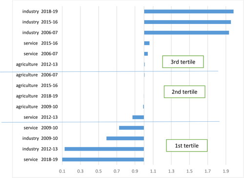
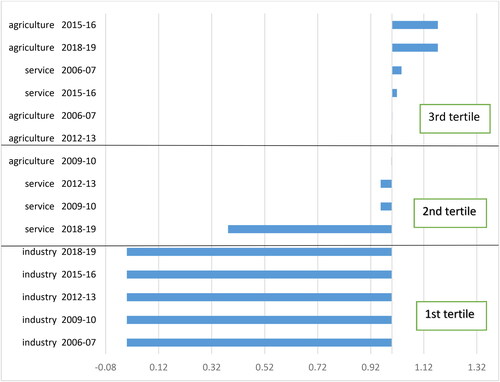
The current study applied the dataset of agriculture, services, and industrial sectors of Pakistan during the period of 2006–2019 to evaluate the energy-based CO₂. In Figure 1, we captured the structure effect in three sectors. The results indicated that the structure affects the agriculture sector in 2nd tertile, which is an average performance in different periods. The economic reason for the performance of the agriculture sector is average because the government policy focuses on the growth of the agriculture sector by helping small-scale farmers, marginalizing farmers, and introducing innovative, environmentally friendly technologies. The government provides cheap environment-friendly machinery for agro tube wells and awareness of efficient use of water, which reduces the energy consumption in the agriculture sector. As a result, this sector’s overall performance is increased. The reason is that, in Pakistan, most of the community is, directly and indirectly, related to the agriculture sector; they use a simple production method. CO₂ emissions, while in the industrial and transport sectors, both exist in 3rd tertile of below-average performance in 2006–07, 2015–16, and 2018–19. While in other, two-study time they fall in 1st tertile of above-average performance.

Figure 1. Structure effect of carbon decomposition identification.

Source: author’s calculation

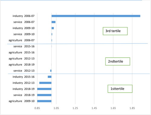
In the case of the intensity effect (Figure 2), all three sectors have mixed results. The agriculture sector almost exists in 2nd tertile, as in the case of the intensity effect, while the industry and service sectors show different results. In the initial period of study, service and industry both of these sectors existed in 3rd tertile, e.g. (2006–07), while in the case of 2012–13, both fell in 1st tertile and the industry sector in 1st tertile, while servicing sector in 2nd tertile 2015–16. While in the 2018–19 period, they exist in 1st tertile. Nevertheless, the overall findings indicate that there has been an improvement in the performance of the various sectors, as seen by the fact that their most recent year’s performance places them in the second and first tertiles, respectively.

Figure 2. Intensity effect of carbon decomposition identification.

Source: author’s own calculation

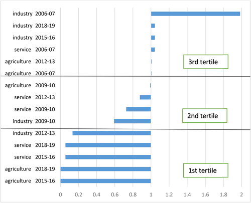
The third element, which can be seen in Figure 3, is the production GDP gap effect. It compares prospective economic outputs to real economic outputs and also considers the economic efficiency of production. The service sector during 2015–16 and 2018–2019 had above-average performance, while in other periods, it fell in the second and 3rd tertile. While in case of the industrial sector, it showing mixed results by existing in 3rd tertile in 2006–07, 2015–16, and 2018–19, whereas in 2009–10 and 2012–13, it exists in 1st tertile. It illustrates that by the time the manufacturing part is still incompetent after 2012–13 in output. While in the case of the agriculture sector, once again, it falls 2nd tertile during the first and second observation periods and moves to 1st tertile in 2015–16.

Figure 3. Production gap effect of carbon decomposition identification.

Source: Author’s Calculation

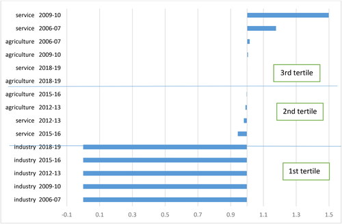
Figure 4 indicates the energy use productivity effect in three sectors. In contrast, in the case of energy, the custom effectiveness effect (ΔEUP) in the manufacturing segment shows average performance by existing in 1st tertile. In contrast, the agriculture and service sector remains in the same area, and both these sectors continued in 3rd tertile in 2006–07, 2009–10 while moving to 2nd tertile in 2012–13 and 2015–16 (Figure. 4). This term consists of energy use technological effect, and energy use technical efficiency change effect, which shows that by the time, the economy of Pakistan is moving through technological advancement.

Figure 4. Energy use productivity effect of carbon decomposition identification.

Source: Author’s Calculation

In Figure 5, the economic efficiency effect is captured. In the end, the fifth factor is the Economic Efficiency Effect (ΔEE) which is premeditated through the shepherd distance parameter to check the economic output efficiency. On the other hand, the industrial sector is in 1st tertile, and the service sector exists second and 3rd tertile. Years 2012–13 and 2015–16 both remain in the 2nd tertile; however, in the study period, both fall in the 3rd tertile of the below-average performance.

Figure 5. Economic efficiency effect of carbon decomposition identification.

Source: Author’s Own Calculation

Considering the objective mentioned above, the empirical evaluation of this study shows that the agriculture sector has an average level of performance due to the structure effect, while CO₂ emission is below the average line due to the industrial and transport sector. For the intensity effect, the response of the underlined sectors is mixed. According to the production GDP gap effect, this factor considers the economic efficiency of production in addition to comparing the expected economic outputs to actual economic outputs. Likewise, the energy use productivity effect of carbon decomposition identification which covered the impact of technological innovation in energy use and technological innovation in energy efficiency, demonstrates that the economy of Pakistan is adapting to the changing technological landscape. Finally, the economic efficiency effect of carbon decomposition identification shows that the industrial, agriculture, and service sector perform averagely in the 1st tertile; however, the former two performances shifted below average in the third tertile.

4. Conclusion

This study evaluates the relative performance of Pakistani industries in terms of CO₂ emissions intensity throughout considering the longitudinal data set till the current periods. For this purpose, we have considered data started from 2006 to 2019 for a comprehensive comparison of results. Our study also considers nine components translated into five factors: intensity impact, energy, utilization productivity effect, output gap effect, structure effect, and ideal output production effect to decide which sectors function better or worse. The overall performance of structure-effect decompositions is unsatisfactory. Most of the sectors spent the previous session in the second and third tertial positions. As a result of the intensity outcome impact, most of the units in 2018–2019 are in the first and second tertiles, and they are continuously moving into the first tertile as energy consumption per unit of GDP decreases, which may have an impact on carbon degradation. In the case of the GDP gap effect, the performance level of the agriculture and service sectors is strong. However, the progress of the industrial sector shows some signs of flagging. The industrial sector has become significantly efficient due to technological advancements and a more advanced production process due to the post-millennium industrialization boom.

4.1. Policy suggestions

The following are significant policy recommendations for Pakistan’s economy based on the discussion: First, energy practice structural and output effects substantially impact on the production of carbon. Therefore, Pakistan’s output-production technology must be enhanced. The government should prioritize technological advancement and technology transfer from technologically advanced nations. For these regions, policymakers should focus on energy consumption efficiency through technological advancements or implement a plan that boosts output and energy efficiency. Establishing an energy commission that considers the region’s energy consumption and output is one feasible option that optimizes energy usage structure and increases energy production in Pakistan. The second significant source of carbon emissions is the intensity impact and energy consumption efficiency. Therefore, policies must prioritize energy-related technical efficiency to reduce CO₂ emissions. Thus, sufficient efforts should be made to enhance the technical efficiency of energy consumption. CO₂ emissions taxation could be another method of policy in Pakistan. As the economic policies of Pakistan are under the umbrella of the China-Pakistan Economic Corridor (CPEC) program, it should provide ambitious energy and infrastructural projects.

Energy projects, particularly coal-related ones, put a significant impact on the amount of carbon dioxide released into the atmosphere. The decomposition analysis assists the government and other stakeholders in finding a balance between the requirements for energy, the potential for economic growth, and the effects of climate change.

This study can be expanded upon in various ways by future research: To begin, the proposed spatially integrated framework applies not just to comparisons of CO₂ emissions on a sectoral level but also on a providence level, as well as on a national level of performance. It is because the framework is flexible enough to accommodate both of these levels of analysis. In addition to the currently conducted study at the level of individual sectors, the proposed methodology is also applicable at the level of the entire economy. Second, we reconnoitered the broad industries such as manufacturing, agriculture, and services. In subsequent research, these sectors might be broken down further into others, such as the manufacturing and financial sectors, covering the totality of Pakistan.

Disclosure statement

No conflict of interest has been reported by the authors.

References

- Ali, R., Ishaq, R., Bakhsh, K., & Yasin, M. A. (2022). Do agriculture technologies influence carbon emissions in Pakistan? Evidence based on ARDL technique. Environmental Science and Pollution Research, 29(28), 43361–43370. https://doi.org/10.1007/s11356-021-18264-x
- Arora, N. K., & Mishra, I. (2021). COP26: More challenges than achievements. Environmental Sustainability, 4(4), 585–588. https://doi.org/10.1007/s42398-021-00212-7
- Azam, M., Liu, L., & Ahmad, N. (2021). Impact of institutional quality on environment and energy consumption: Evidence from developing world. Environment, Development and Sustainability, 23(2), 1646–1667. https://doi.org/10.1007/s10668-020-00644-x
- Azam, M., Nawaz, S., Rafiq, Z., & Iqbal, N. (2021). A spatial-temporal decomposition of carbon emission intensity: A sectoral level analysis in Pakistan. Environmental Science and Pollution Research, 28(17), 21381–21395. https://doi.org/10.1007/s11356-020-12088-x
- Bartoletto, S., & Rubio, M. (2008). Energy transition and CO2 emissions in Southern Europe: Italy and Spain (1861–2000). Global Environment, 1(2), 46–81. https://doi.org/10.3197/ge.2008.010203
- Chung, Y. H., Färe, R., & Grosskopf, S. (1997). Productivity and undesirable outputs: A directional distance function approach. Journal of Environmental Management, 51(3), 229–240. https://doi.org/10.1006/jema.1997.0146
- Ding, T., Huang, Y., He, W., & Zhuang, D. (2021). Spatial–temporal heterogeneity and driving factors of carbon emissions in China. Environmental Science and Pollution Research, 28(27), 35830–35843. https://doi.org/10.1007/s11356-021-13056-9
- Ding, W., Levine, R., Lin, C., & Xie, W. (2021). Corporate immunity to the COVID-19 pandemic. Journal of Financial Economics, 141(2), 802–830. https://doi.org/10.1016/j.jfineco.2021.03.005
- Du, K., Xie, C., & Ouyang, X. (2017). A comparison of carbon dioxide (CO2) emission trends among provinces in China. Renewable and Sustainable Energy Reviews, 73, 19–25.
- Färe, R., Grosskopf, S., Lindgren, B., & Roos, P. (1994). Productivity developments in Swedish hospitals: a Malmquist output index approach. In Data envelopment analysis: Theory, methodology, and applications (pp. 253–272). Dordrecht: Springer. https://doi.org/10.1007/978-94-011-0637-5_13
- Gazheli, A., Van Den Bergh, J., & Antal, M. (2016). How realistic is green growth? Sectoral-level carbon intensity versus productivity. Journal of Cleaner Production, 129, 449–467. https://doi.org/10.1016/j.jclepro.2016.04.032
- Hina, S., Saleem, F., Arshad, A., Hina, A., & Ullah, I. (2021). Droughts over Pakistan: Possible cycles, precursors and associated mechanisms. Geomatics, Natural Hazards and Risk, 12(1), 1638–1668. https://doi.org/10.1080/19475705.2021.1938703
- International Energy Agency. (2020). Renewables—Global Energy Review 2020—Analysis—IEA. Iea
- Jiang, Z., Ding, Z., Liu, Y., Wang, Y., Hu, X., & Yang, Y. (2020). A data-driven based decomposition–integration method for remanufacturing cost prediction of end-of-life products. Robotics and Computer-Integrated Manufacturing, 61, 101838. https://doi.org/10.1016/j.rcim.2019.101838
- Lin, B., & Ahmad, I. (2017). Analysis of energy related carbon dioxide emission and reduction potential in Pakistan. Journal of Cleaner Production, 143, 278–287. https://doi.org/10.1016/j.jclepro.2016.12.113
- Lin, B., & Du, K. (2014). Decomposing energy intensity change: A combination of index decomposition analysis and production-theoretical decomposition analysis. Applied Energy, 129, 158–165. https://doi.org/10.1016/j.apenergy.2014.04.101
- Liu, X., Zhou, D., Zhou, P., & Wang, Q. (2018). Factors driving energy consumption in China: A joint decomposition approach. Journal of Cleaner Production, 172, 724–734. https://doi.org/10.1016/j.jclepro.2017.10.238
- Nag, S., Hughes, S. P., & Le Moigne, J. (2016). Streamlining the design tradespace for Earth imaging constellations. In AIAA SPACE 2016 (p. 5561). https://doi.org/10.2514/6.2016-5561
- Pant, H., Verma, J., & Surya, S. (2020). Environmental issues: Local, regional, and global environmental issues. Environmental issues: Local, regional, and global environmental issues, 234–246.
- Pasurka, C. A. (2006). Decomposing electric power plant emissions within a joint production framework. Energy Economics, 28(1), 26–43. https://doi.org/10.1016/j.eneco.2005.08.002
- Paz-Kagan, T., Ohana-Levi, N., Herrmann, I., Zaady, E., Henkin, Z., & Karnieli, A. (2016). Grazing intensity effects on soil quality: A spatial analysis of a Mediterranean grassland. CATENA, 146, 100–110. https://doi.org/10.1016/j.catena.2016.04.020
- Samuwai, J., & Hills, J. M. (2018). Assessing climate finance readiness in the Asia-Pacific region. Sustainability (Switzerland), 10(4), 1192. https://doi.org/10.3390/su10041192
- Sheinbaum, C., Ozawa, L., & Castillo, D. (2010). Using logarithmic mean Divisia index to analyze changes in energy use and carbon dioxide emissions in Mexico’s iron and steel industry. Energy Economics, 32(6), 1337–1344. https://doi.org/10.1016/j.eneco.2010.02.011
- Su, B., & Ang, B. W. (2012). Structural decomposition analysis applied to energy and emissions: Some methodological developments. Energy Economics, 34(1), 177–188. https://doi.org/10.1016/j.eneco.2011.10.009
- Sun, J. W. (1998). Changes in energy consumption and energy intensity: A complete decomposition model. Energy Economics, 20(1), 85–100. https://doi.org/10.1016/S0140-9883(97)00012-1
- Villa, F., Bagstad, K. J., Voigt, B., Johnson, G. W., Portela, R., Honzák, M., & Batker, D. (2014). A methodology for adaptable and robust ecosystem services assessment. PLoS One. 9(3), e91001. https://doi.org/10.1371/journal.pone.0091001
- Wang, H., Ang, B. W., & Zhou, P. (2018). Decomposing aggregate CO2 emission changes with heterogeneity: An extended production-theoretical approach. Energy Journal, 39(1). https://doi.org/10.5547/01956574.39.1.hwan
- Wang, J. W. (2020). Spatial domain decomposition approach to dynamic compensator design for linear space-varying parabolic MIMO PDEs. IET Control Theory and Applications, 14(1), 39–51. https://doi.org/10.1049/iet-cta.2019.0404
- Wang, Q., Chiu, Y. H., & Chiu, C. R. (2015). Driving factors behind carbon dioxide emissions in China: A modified production-theoretical decomposition analysis. Energy Economics, 51, 252–260. https://doi.org/10.1016/j.eneco.2015.07.009
- Wang, Q., Hang, Y., Su, B., & Zhou, P. (2018). Contributions to sector-level carbon intensity change: An integrated decomposition analysis. Energy Economics, 70, 12–25. https://doi.org/10.1016/j.eneco.2017.12.014
- Wei, W., Zhang, X., Cao, X., Zhou, L., Xie, B., Zhou, J., & Li, C. (2021). Spatiotemporal dynamics of energy-related CO2 emissions in China based on nighttime imagery and land use data. Ecological Indictors, 131, 108132.
- Xu, S. C., Zhang, L., Liu, Y. T., Zhang, W. W., He, Z. X., Long, R. Y., & Chen, H. (2017). Determination of the factors that influence increments in CO2 emissions in Jiangsu, China using the SDA method. Journal of Cleaner Production, 142, 3061–3074. https://doi.org/10.1016/j.jclepro.2016.10.161
- Zhou, P., & Ang, B. W. (2008). Decomposition of aggregate CO2 emissions: A production-theoretical approach. Energy Economics, 30(3), 1054–1067. https://doi.org/10.1016/j.eneco.2007.10.005