Estimating the effect of long-term mechanism for real estate in China: a regression discontinuity approach

Abstract

Housing prices in China have risen dramatically in recent decades, giving rise to bubble concerns. Many studies show that short-term regulation of real estate market is ineffective, which drove central government to propose the construction of a long-term mechanism for real estate in late 2016. However, few studies have been conducted to estimate its effects. This article highlights the effects of the long-term mechanism on housing prices, similar to a quasi-natural experiment, with the proposal of the long-term mechanism. In this context, the study was conducted with the end of 2016 as a breakpoint, using the RDiT method and panel data for 35 large- and medium-sized cities from 2009 to 2021, to find out whether the long-term mechanism has stabilized housing prices or not. The results reveal that the long-term mechanism dramatically reduced the divergence and dispersion of housing prices from the long-term equilibrium level. Further study shows that there is significant heterogeneity in the impact of the long-term mechanism on housing prices across cities, with significant effects in second-tier cities but not in first-tier cities, and with significant effects in central and western cities but not in eastern cities. Therefore, we suggest that the eastern, including the first-tier cities, remain the focus of the construction of the long-term mechanism in the future, and continue to implement short-term regulation for key cities, and build a system that coordinates with the long-term mechanism.

Keywords:

• Real estate
• long-term mechanism
• regression discontinuity

JEL classification:

• E32
• E61
• G38

1. Introduction

The regulation train of thought has gone through two periods since 2003, when the central government identified the real estate industry as a pillar of the national economy. The previous one prior to 2016 was characterized by a short-term emphasis and demand suppression. Despite the fact that the central government implemented many rounds of housing price regulation, the consequences were mostly negative (Chen et al., 2018). Housing prices are stuck in a dilemma of rising with more regulation as the real estate market continues to deviate from its equilibrium. The central government explicitly proposed a long-term mechanism for real estate for the first time at the Central Economic Work Conference (CEWC) in December 2016, signaling a shift in the train of thought toward the establishment of a basic and long-term system for the real estate market. Obviously, unlike the single policy of the past, the long-term mechanism is the combination punch, including both existing regulatory policies and a series of urgently needed systems (or rules), the purpose of which is to stabilize the real estate market in the long run, not just to suppress housing prices.

Under the pressure of further rising housing prices since the first half of 2016, the central government still introduced short-term regulatory policies with unique Chinese characteristics, including property-purchasing limitation, credit restriction and so on. Purchasing limitation is the most severe means of administrative intervention in the real estate market. Its aim is to curb investment and speculative demand by limiting the number of housing purchases by local residents and migrants. Usually, in conjunction with purchasing limitation, credit restriction is implemented by the means of limiting the down payment ratio, differentiating the interest rate policies. As a result, the growth rate of housing prices in first- and second-tier hot cities slowed down significantly in 2017, but in the long run, it is lack of sustainability (Chen et al., 2018). Therefore, the central government, consistently put forward deployments and requirements for the establishment of a long-term regulation system for real estate in the two sessions¹ and CEWC since 2017. It shows that the central government is committed to ensuring the healthy and stable development of the real estate market in order to ensure its long-term sustainability.

It has been five years since the implementation of the long-term mechanism. Undoubtedly, it has great theoretical and practical significance to clarify the effect of its implementation, and whether it has promoted the stable and healthy development of the real estate market. At the 2020 real estate symposium, Vice Premier Han Zheng believed that the long-term mechanism for real estate had been put in place and the results achieved deserve recognition, and requested a summary of the implementation. However, Due to the ineffectiveness of curbing the rise in housing prices, 12 city mayors were interviewed in 2018, and call roll alerts to ten city governments were conducted in 2019, by the Ministry of Housing and Urban-Rural Development of the People’s Republic of China (MOHURD). Evidently, the two facts mentioned above show that the construction of the long-term mechanism is clearly differentiated at the local government level Therefore, it is necessary to objectively assess the effects of the long-term mechanism in different cities, so as to provide a basis for the central government to supervise local governments and promote city-specific policies.

Most relevant studies in China are about the reasons for the failure of central government macro-control prior to 2016, such as Han and Jiang (2011), Zhu and Yan (2013), Wang and Hou (2017), Chen et al. (2018), and Zheng and Yan (2021). Other current researches, directly related to the long-term mechanism, mainly focuses on how to build and improve, specifically, describing the objectives, connotations, composition, and implementation path of the long-term mechanism, such as Huang et al. (2018). However, a review of the literature revealed no studies on the effect evaluation of the long-term mechanism for real estate.

This study contributes to the literature in the following ways. First, unlike the existing literature, which mostly studies the construction and improvement of the long-term mechanism, the study in this article focuses on the effect of the long-term mechanism on housing prices. Second, the study was conducted with the proposal of the long-term mechanism as a breakpoint, using the RDiT method to find out whether the long-term mechanism has stabilized housing prices or not. Third, the study provides empirical evidence on the heterogeneity cross cities, which would help the central government to more specifically supervise the local governments to build and improve the long-term mechanism.

2. Analysis on the implementation background and connotation of the long-term mechanism for real estate in China

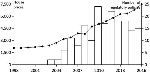
Figure 1 depicts the trend in housing prices and the severity of regulatory policies from 1998 to 2016. China’s real estate market reform began in 1998. Prior to 2003, housing prices across the country were relatively stable, but after the central government implemented macro-control in 2003, housing prices across the country continued to rise sharply, except for a brief decline in 2008 due to the financial crisis. After 2008, the central government interfered in the real estate market more intensively and frequently (see the right axis of Figure 1), but the rise in housing prices was still unabated. Although the central government’s policy regulation cannot simply be attributed as the direct cause of rising housing prices, various studies in the literature show that it is an essential factor (Chen & Yang, 2013; Tan & Wang, 2015; Zheng & Yan, 2016; Zhou & Wu, 2008; Zong et al., 2010). Scholars have undertaken various research on the relationship between policies and housing prices as to why regulatory policies have failed. Both academia and government have increasingly agreed that the central government’s regulatory policies lack dynamic consistency and foresight for a long period (Han & Jiang, 2011; Xu, 2012). The reason is that most regulatory policies rely on administrative tools like purchase limits and credit restrictions, which are ineffective with only short-term impact (Chen, 2018b). With the soaring housing prices in first-tier and some second-tier cities² in the first half of 2016, the call for building a long-term mechanism for real estate was unprecedentedly high (Chen, 2018b), which was then formally proposed by the central government at the CEWC in December of the same year.

Figure 1. Trend of housing prices and the intensity of central government regulatory policies, 1998-2016.

Note: The left axis represents housing prices, data from the CEI database. The right axis represents the number of real estate regulatory policies (only those at the central government level are counted), as determined by the text of previous year’s central government regulations.

Source: data from CEI (China Economic Information Network) database.

The CEWC's announcement in December 2016 on the long-term mechanism for real estate was more formally launched in three respects.

First, it established a clear position: houses are for living in, not for speculating. Residents of China have seen a major improvement in their living conditions as a result of market-oriented reforms, with per capita housing floor area of urban residents reaching 36.6 m² in 2016, already close to the level of the UK and Japan. However, the dramatic rise in housing prices in China after 2000, as well as the resulting bubble, cannot be attributed simply to local demand. Numerous studies have revealed that there is a significant element of investment and speculation in the real estate market (Tan & Wang, 2015; Zheng & Yan, 2016). Guided and driven by the expectation of rising housing prices in the market, social capital has been taking the real estate market as the best investment choice (Guo & Huang, 2018). However, short-term issues such as monetary policy, financial development, and soft credit limits are also significant contributors to the excessive rise in housing prices (Zhou, 2006). Therefore, the basis for building the long-term mechanism is to return housing to its residential function, and the key is to cut off the space for housing speculation.

Second, it set precise objectives: curbing the real estate bubble and avoiding big ups and downs. Stability has always been the central government’s goal for the real estate market. Unlike in the past, the 2016 CEWC and subsequent policy texts have gradually formed a clear goal of three stability: stable home prices, stable land prices, and stable expectations. According to several studies on real estate bubbles (Kuang, 2010; Shiller, 2005; Zhang et al., 2020), investor expectations have a substantial impact on housing price volatility and bubbles. Jia and Li (2013) present strong evidence that between 2002 and 2011, noise traders’ expectations were a major source of housing price volatility and bubbles, but regulatory policies imposed by the central government have had little effect. The reason is that under the short-term, one-size-fits-all and repeated and variable policies, it is difficult for investors to form correct and stable expectations, and they can only blindly follow the herd.

Third, it constructed a independent framework: a system integrating financial, land, fiscal and tax, investment, and legislative instruments. Taking stable growth as its primary goal, past real estate regulation was essentially subordinate to macro-control (Chen, 2018a). where the means used, such as monetary policy, fiscal policy, etc., were different from those used for, but also used for real estate regulation. For example, the financial policy of targets interest rates of housing loan in real estate regulation, while targets all loans in macro-control. The new expression obviously connotes the independence of the above-mentioned means in real estate regulation, and stable house prices has also become the inherent meaning. Thus, under the status of independence and the goal of stable housing prices, real estate regulation can ensure long-term stability and truly build up a long-term mechanism for real estate. (Chen, 2018a).

Obviously, the proposed long-term mechanism focuses on the key to a long-term mechanism for real estate: long-term effect (Chen, 2018a). The next institutional reforms by the central government in 2017, including the rental market, land supply, and financial regulation, marked the full implementation phase of the long-term mechanism for real estate. Therefore, given the proposal of the long-term mechanism for real estate in late 2016 similar to a quasi-natural experiment, this study employs the RD method to estimate the effect of it on housing prices, with the end of 2016 as the breakpoint and the post-2016 sample as the treatment group.

3. Empirical strategy and econometric model

3.1. Empirical strategy

In contrast to the natural sciences, such as epidemiology and biostatistics, the social sciences, such as economics, have struggled to organize clinical trials, preventing causal inference from becoming widespread in the field of economics. After 2000, extensive studies on government policies conducted by the MIT Poverty Alleviation Laboratory (J-PAL), made randomized controlled trials (RCTs) the ideal form of policy evaluation, and a series of methods for evaluating policy effects based on causal inference emerged, including instrumental variable (IV), difference-in-differences (DID), propensity matching (PM), and regression discontinuity (RD). In policy evaluation, the IV approach can effectively deal with endogeneity. The difficulty, however, is in determining the best instrumental variable. Meanwhile, in order to identify ATT and ATE, the researcher have to disregard the heterogeneity of the research subject (Heckman, 1997). The DID method has been widely used because it allows for the presence of unobservable and relaxes the conditions for policy evaluation However, the DID method has obvious limitations, such as stricter data requirements, failure to account for individual time-point effects, and environmental influence effects. The PM approach includes covariate matching (CVM) and propensity score matching (PSM), with PSM being the most commonly used method in policy evaluation. But its application requires the assumption of strong negligibility (Kannika et al., 2010) and a large amount of individual data, which affects its accuracy. RD, proposed by Campbell (1958), wasn’t applied in economics until Hahn et al. (2001) offered theoretical proofs and estimating methods. The RD approach is the most credible of the quasi-experimental methods in two ways: first, it can avoid endogeneity concerns in parameter estimation; second, it can readily test the important hypothesis that individuals at the breakpoint have the same characteristics (Lee & Lemieux, 2010).

According to available studies, a certain degree of bubble had accumulated in the Chinese real estate market before 2016 (Gao et al., 2014; Li, 2015; Lv, 2010). Housing prices bubble, defined by Blanchard and Fischer (1989) as an excess of prices over economic fundamentals, can thus be described as an excess of housing prices over underlying values, or a divergence of housing prices from long-term equilibrium prices. Large fluctuations in housing prices in short-term will create room for arbitrage and a significant increase in the speculative component of the market, which will not only cause a crowding-out effect on rigid demand, but will also cause a large number of resources to flow to the real estate market, and have a crowding-out effect on the real economy. Furthermore, continued imbalance in housing prices could also destabilize the financial sector, and bring about a more serious crisis. The goal of the central government in building the long-term mechanism is to smooth out short-term deviations in housing prices from underlying values, and to keep housing prices converging to economic fundamentals in the long run. Therefore, evaluating the effect of the long-term mechanism also means whether the deviation of housing prices from long-term equilibrium values has been effectively controlled after the implementation of the long-term mechanism compared to the pre-2016 period.

The following constraints are considered in method selection. First, IV method can be used in response to endogeneity concerns in observational data, with lagged variables as instrumental variables. But it is difficult to meet two conditions characterized by Bellemare et al. (2017) in real estate market, these are (i) serial correlation in the potentially endogenous explanatory variable and (ii) no serial correlation among the unobserved sources of endogeneity. So, the estimates of parameters by IV method are hard to be valid. Second, due to short implementation time of the long-term mechanism for real estate, it is not easy to construct a long series sample. Third, this article needs to consider the individual effects of the study subjects. As a result, this study employs the RD approach to examine the potential breakpoints signaled by the official start of the long-term mechanism for real estate in late 2016. The main notion of RD is that, following a pre-defined rule, samples are assigned to both sides of the breakpoint formed by the exogenous regime, which would lead to the effect of the local randomized trial near the breakpoint, and achieve causal identification. (Jin et al., 2020).

3.2. RD model and RDiT research framework

The OLS approach would be valid to estimate the causal influence of the long-term mechanism on housing prices if complete randomness is satisfied, but it is difficult to satisfy in practice. This is because some factors that affect both the outcome and treatment variables may not be observed at all, thus resulting the problem of omitted variables; In addition, the degree of housing price deviation may also affect the implementation effect of the long-term mechanism, i.e., there is reverse causality. Thus, the model endogenous problem, caused by the above two conditions makes the OLS estimate no longer valid. The official introduction is similar to conduct a randomized trial to implement the long-term mechanism, and all samples are divided by breakpoints into a treatment group that is subjected to policy intervention and a control group that is not. Compared to the OLS, the RD method, using the breakpoint as an instrumental variable to enter the treatment group, is able to solve possible endogeneity problems. The RD model might be expressed as Eqs. (1)(1) $$Y_i=\alpha +\beta D_i+f\left(\mathit{tim}{e}_i\right)+{\epsilon }_i$$(1) to (2)(2) $$D_i=\{\begin{array}{c}1\mathit{\text{ if }}{\mathit{time}}_i > T_0\\ 0\mathit{\text{ if }}{\mathit{time}}_i \le T_0\end{array}$$(2) . (1) $$Y_i=\alpha +\beta D_i+f\left(\mathit{tim}{e}_i\right)+{\epsilon }_i$$(1) (2) $$D_i=\{\begin{array}{c}1\mathit{\text{ if }}{\mathit{time}}_i > T_0\\ 0\mathit{\text{ if }}{\mathit{time}}_i \le T_0\end{array}$$(2) Here $Y_i$ is the outcome variable. ${\mathit{time}}_i$ is the driver variable, which indicates the time the sample is in, $D_i$ is the treatment variable, indicating whether the long-term mechanism is implemented ($D_i$=1, yes; $D_i$=0, no), and is a discontinuous function of ${\mathit{time}}_i.$ $T_0$ is the breakpoint, indicating the time when the long-term mechanism was officially proposed, that is, late in 2016.

According to the mechanism of allocation processing at breakpoints, RD can be divided into Sharp RD and Fuzzy RD, Eq. (2)(2) $$D_i=\{\begin{array}{c}1\mathit{\text{ if }}{\mathit{time}}_i > T_0\\ 0\mathit{\text{ if }}{\mathit{time}}_i \le T_0\end{array}$$(2) describes a situation in which the exact breakpoint is returned—D_i is assigned exactly according to the breakpoint. We assume in this study that near the breakpoint, all sample cities implement the long-term mechanism, with a mutant relationship from 0 to 1, so the Sharp RD approach is used for the next analysis.

Most existing studies on RD application use the standard cross-sectional framework, but in recent years, increasing empirical work has adapted the RD to applications where time as a running variable and treatment begins at a particular threshold in time (Hausman & Rapson, 2018), a framework known as RDiT (regression discontinuity in time). The deployment of RDiT faces a number of challenges, due primarily to its reliance on time-series variation for identification. There are three potential pitfalls linked with the RDiT framework, according to Hausman and Rapson (2018).

First, RDiT is often used with no or insufficient cross-sectional identifying variation, the sample is too small as the bandwidth narrows around the breakpoint. Thus, the RDiT can only expand the time dimension $T,$ i.e., using samples away from the breakpoint, to obtain sufficient power, which would lead to bias resulting from unobservable confounders and/or the time-series properties of the data generating process.

Second, due to the nature of underlying data generating process, time-series data used in RDiT, can result in autoregressions in the explanatory variables, which would affect the estimation of short- and long-term effects.

Third, when time is the running variable, the McCrary density test fails, which make it difficult to assess if the samples have sorted across the breakpoint.

This study incorporates control variables into the RDiT model, as suggested by Hausman and Rapson (2018), not only to reduce noise and improve precision, but also to avoid estimate bias. A local linear context is used to compare model selection. Annual panel data, as well as cross-sectional variance, are employed in data selection to reduce estimation bias even more. Placebo, heterogeneity, and multiple bandwidth tests are conducted to increase the robustness of the RDiT model.

Thus, this study derives Eq. (3)(3) $$Y_i={\beta }_0+{\beta }_1{D}_i+{\beta }_{2}f\left(T_i\right)+\phi X_i+\mathit{cit}{y}_i+{\mu }_i$$(3) to assess the impact of ${\mathit{time}}_i=T_0(2016)$ at $D_i$ (the long-term mechanism) on $Y_i$ (outcome variable). (3) $$Y_i={\beta }_0+{\beta }_1{D}_i+{\beta }_{2}f\left(T_i\right)+\phi X_i+\mathit{cit}{y}_i+{\mu }_i$$(3)

Here, $\mathit{cit}{y}_i$ is a dummy variable for the city where the sample is located to control for city fixed effects. $X_i$ is the control variables for economic fundamentals. $f(·)$ is the local smoothing function of the variables $T_i,$ a nonlinear function expressed as a $\text{polynomial in T w}$ ith second-order³, according to Gelman and Imbens (2019) and Jin et al. (2020). Due to the heterogeneity of the long-term mechanism implementation, the results of the RDiT estimate is a Local Average Treatment Effect (LATE), which is the parameter ${\beta }_1$ in Eq. (3)(3) $$Y_i={\beta }_0+{\beta }_1{D}_i+{\beta }_{2}f\left(T_i\right)+\phi X_i+\mathit{cit}{y}_i+{\mu }_i$$(3) .

The following three estimation method were chosen for comparison: (1) RD non-parametric estimation; (2) OLS linear estimation; and (3) 2SLS instrumental variable linear estimation. To deal with the variable $D_i,$ this study defines $T_i=1$ (${\mathit{time}}_i>T_0$) as the instrumental variable (i.e., $T_i$ takes the value of 1 after $T_0$ and 0 otherwise). $T_i$ is valid and delivers consistent estimation results since it meets the correlation and exogeneity conditions between $T_i$ and $D_i.$

4. Data sources and variable selection

4.1. Data sources

The research object of this study are 35 large- and medium-sized cities from 2009 to 2021. Annual panel data would be helpful for this study in three aspects. First, compared to time-series data in RDiT framework, panel data can reduce bias to a certain extent and avoid endogenous problems. Second, because of obvious heterogeneity across cities, it is important for the construction of the long-term mechanism for real estate to implement city-specific and no one-size-fits-all policies. According to many research (Zheng, 2019), housing price bubbles are mostly found in first- and second-tier cities, which are also the key pilot ones for the implementation of the long-term mechanism, Therefore, taking 35 large- and medium-sized cities as a sample can more objectively reflect the implementation effect of the long-term mechanism. Third, following the subprime mortgage crisis in 2009, the central government frequently adopt short-term regulatory policies in the real estate market. Since then, in addition to the change in the central government’s regulation toute, the external environment of the real estate market has remained basically the same, which provides a better precondition for RD analysis.

The sample size is 455, with 175 in the treatment group and 280 in the control group. The data are from the National Bureau of Statistics, CEI, and Statistical Yearbook by Cities.

4.2. Selection of variables

The dependent variable in this study is hp, measuring the extent to which housing prices deviate from their equilibrium levels. Learning from the practices of Tan and Wang (2015), hp equals to the balance of the actual and the equilibrium housing prices divided by the latter. Among them, housing prices equal to total sales of commercial housing divided by its overall area, and the equilibrium housing prices are obtained by HP filter method. Furthermore, we use another dependent variable housing price bubbles (hpb) as a comparative one for hp, which is calculated the same way as hp. The difference is that, the equilibrium housing prices are obtained through the fundamental price model proposed by Abraham and Hendershott (1994), in which the equilibrium housing prices are determined by a range of variables.

This study divides control variables into two group, one is economic fundamental variables and the other is real estate market ones. In many studies, economic fundamentals can adequately explain housing prices (Capozza et al., 2002; Hort, 1998; Hort, 1998), which in the long term mainly reflect economic fundamentals (Mcquinn & O'reilly, 2008). Based on the studies of Shen and Liu (2004), Yu (2010), Chen (2018), and Zheng, (2020), per capita disposable income ($\mathit{income}$), leverage ratio ($\mathit{loan}$), total urban population ($\mathit{pop}$), long-term real interest rate ($\mathit{rate}$), and local fiscal expenditure ($\exp$) are chosen as economic fundamentals. Among them, $\mathit{loan}$ is equal to the ratio of loans balance of financial institutions at year-end to real GDP, taking 1999 GDP as the base period real GDP, and on the basis of the actual GDP of the previous year, multiplying by the GDP index of the current year to calculate the real GDP of the current year. According to the practice of Chen and Fu (2013), $\mathit{rate}$ is equal to the 5-year fix mortgage rates, weighted by the number of days before and after the adjustment day in the year in which the interest rate is adjusted, minus the current inflation rate. $\exp$ is described as the local budget expenditure. We set variables of the real estate market in the two aspects of development and transaction, using total investment in real estate development ($\mathit{invest}$) and real estate construction area ($\mathit{cons}\_\mathit{area}$) to characterize the capital investment and physical construction in real estate development, and using area of apartment sales ($\mathit{sales}\_\mathit{area}$) and land acquisition area ($\mathit{land}\_\mathit{area}$) to characterize the transactions in the commercial housing market and the land markets, respectively.

The year 2009 was chosen as the base period, and all price-based variables were deflated based on the Consumer Price Index ($\mathit{cpi}$) to exclude the impact of inflation. And all absolute variables were handled as logarithmic.

The descriptive statistics are shown in Table 1.

Table 1. Descriptive statistics for key variables.

Variables	N	Mean	St. dev	Min	Median	Max
$hp$	455	0.00	0.06	−0.16	0.00	0.30
$\mathit{invest}$		6.64	0.82	4.30	6.71	8.16
$\mathit{cons}\_\mathit{area}$		8.70	0.63	6.80	8.72	10.27
$\mathit{sales}\_\mathit{area}$		6.94	0.92	3.90	6.70	8.81
$\mathit{land}\_\mathit{area}$		5.31	0.98	1.00	5.40	7.70
$\mathit{income}$		10.21	0.32	9.30	10.00	11.00
$\mathit{loan}$		0.89	0.49	0.18	0.66	8.50
$\mathit{pop}$		6.40	0.65	5.10	6.60	8.14
$\mathit{rate}$		3.01	0.93	−0.95	3.20	6.90
$\exp$		6.45	1.00	4.20	6.43	8.79

Source: Authors’ research with original data from the National Bureau of Statistics of China, CEI and China Statistical Yearbook.

The results show that the data distribution of all variables is normal. Compared with hpb calculated by the fundamental price model, hp calculated by the HP filter method is basically the same. Therefore, the results from the HP filter method can be used for empirical analysis.

5. Estimation results and analysis

5.1. City classification by region

There are prominent disparities in population, economic growth and natural endowments between different regions in China. These factors give the real estate market unique geographical features. Therefore, we should analyze the differences in the impact of long-term mechanism on housing prices between different regions.

As shown in Figure 2, according to the regional classification method of the National Bureau of Statistics, and the province, municipality and autonomous region where the city is located, we divide 35 large- and medium-sized cities into three regional cities (eastern, central and western cities). 16 cities are classified as the eastern, including Beijing, Tianjin, Shijiazhuang, Shenyang, Dalian, Shanghai, Nanjing, Hangzhou, Ningbo, Fuzhou, Xiamen, Jinan, Qingdao, Guangzhou, Shenzhen and Haikou. 8 cities are classified as the central, including Taiyuan, Changchun, Harbin, Hefei, Nanchang, Zhengzhou, Wuhan and Changsha. Other 11 cities are classified as the western.

Figure 2. Regions and 35 large- and medium-sized cities in China.⁴

Source: Map data are from DataV.GeoAtlas (http://datav.aliyun.com/portal/school/atlas/area_selector), then edited by the authors.

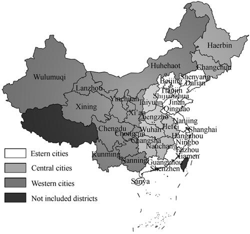
To be precise, the division of the three regions is based on economic policies, other than administrative zoning and geographical boundaries. They do, however, have significant geographical differences. In general, the terrain rises gradually from east to west in China. The most important feature of the eastern is the coast, dominated by plains and hills, and densely populated, 42.05% of the national share (30.75% and 27.2% for the central and western respectively). Guided by a ladder development strategy in the 1980s, the eastern part was the first to implement the opening policy and became a region with the highest level of economic development, 54.4% of the national share (24.8% and 20.8% for the central and western respectively). The western is dominated by plateaus, basins and mountains, vast but sparsely populated in most of areas with less developed economy. The central region, both geographically and economically, is the link between the eastern and the western.

5.2. Breakpoint validity test

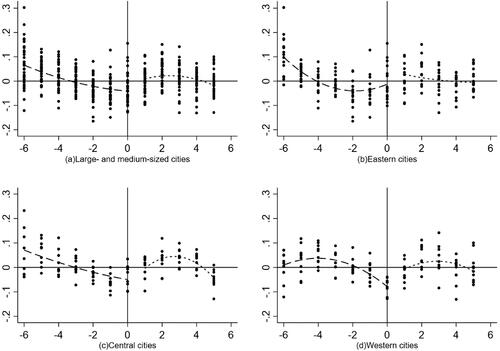
The first step is to establish whether hp has any breakpoints. Figure 3 shows hp of 35 big and medium-sized cities (Figure 2a), eastern cities (Figure 2b), central cities (Figure 2c), and western cities (Figure 2d). As we can see, the eastern and central cities have jumped substantially after 2016. As of 2016, housing prices in all sample cities showed a negative and considerable deviation from the equilibrium level. However, after 2016, housing prices jumped back to the equilibrium level in the eastern and central cities. Although still negatively deviating, the western cities also displayed a jump and a return to equilibrium. Particularly in the central cities, housing prices remained relatively stable around the equilibrium level.

Figure 3. hp for 35 Large- and Medium-sized Cities and Cities in the Eastern, Central and Western.

Source: Authors’ research.

Second, Table 2 displays the RD approach results for continuity. All control variables’ estimated coefficients are not significant at all three bandwidths. This indicates that there is no significant jump in the control variables at the breakpoints, showing that the RD approach is valid.

Table 2. Tests for continuity of control variables.

Bandwidth	income (1)	loan (2)	rate (3)	pop (4)	exp (5)	invest (6)	cons_area (7)	land_area (8)	sales_area (9)
+/-50	0.98 (0.09)	0.39 (0.35)	0.30 (0.35)	0.98 (0.27)	0.97 (0.35)	0.92 (0.31)	0.95 (0.23)	0.81 (0.37)	0.49 (0.28)
+/-100	0.97 (0.09)	0.45 (0.37)	0.35 (0.36)	0.98 (0.28)	0.98 (0.36)	0.91 (0.29)	0.94 (0.24)	0.82 (0.38)	0.46 (0.26)
+/-150	0.94 (0.14)	0.73 (0.58)	0.39 (0.58)	0.99 (0.44)	0.97 (0.26)	0.92 (0.49)	0.95 (0.37)	0.76 (0.27)	0.33 (0.46)

Note: Robust standard errors are in parentheses and clustered to sample cities using clustering robust standard errors. *, ** and *** denote 10%, 5% and 1% significance levels respectively.

Source: Authors’ research.

5.3. Regression results analysis

The breakpoint analysis shows that the optimal bandwidth is 2.5 years. This article customizes three bandwidths for 2, 3, and 4 years. The advantage of a small bandwidth is the ability to control the trend in a lower form, while allowing this trend to differ before and after the breakpoint. However large bandwidths can use as many samples as possible, but require the addition of control variables and higher-order terms. The estimation results of the three methods under three custom bandwidths are presented in Table 3. The results show that the implementation of the long-term mechanism on housing price deviation is positive and significant, and the estimated coefficients are basically close, which indicates that the breakpoint estimation results are valid.

Table 3. Impact of the long-term mechanism implementation on housing prices.

Variables	Dependent variable: hp
Method	RDiT nonparametric estimation			OLS linear estimation			2SLS linear estimation
Bandwidth	+/-2 (1)	+/-3 (2)	+/-4 (3)	+/-2 (4)	+/-3 (5)	+/-4 (6)	+/-2 (7)	+/-3 (8)	+/-4 (9)
Long-term mechanism	0.047*** (0.02)	0.045*** (0.02)	0.039*** (0.01)	0.040** (0.02)	0.055*** (0.02)	0.052*** (0.01)	0.052* (0.03)	0.071*** (0.01)	0.082*** (0.03)
Control variables	Yes	Yes	Yes	Yes	Yes	Yes	Yes	Yes	Yes
Fixed effects	No	No	No	Yes	Yes	Yes	Yes	Yes	Yes
High-order term	Yes	Yes	Yes	No	No	No	Yes	Yes	Yes
F-test				18.32	13.59	12.96	32.83	37.81	17.34
R^2				0.32	0.19	0.24
N	175	245	280	175	245	280	175	245	280

Note: Robust standard errors are in parentheses and clustered to sample cities using clustering robust standard errors. *, **, *** denote 10%, 5%, and 1% significance levels, respectively. 2SLS linear estimation results with F-values are the first-stage F-statistics, and the higher-order terms are quadratic results. The control variables include economic fundamentals and real estate market indicators.

Source: Authors’ research.

The results of non-parametric estimation with higher-order terms controlled are shown in columns 1 to 3, and the coefficient values are basically the same for different bandwidths. The results of the OLS linear estimation are shown in columns 4 to 6, and the values of the optimal bandwidth coefficients are closer to the values of the non-parametric estimation. Columns 7 to 9 show the two-stage least squares (2SLS) estimation, with $T_i=1({\mathit{time}}_i>2016)$ as instrumental variables for the treatment variables. The regression results are significant in the first stage of estimation, which controls for urban dummy variables and a polynomial in time, and the F-values of the instrumental variables are significantly higher than the critical values of the weak instrumental variables (10), which indicates that the instrumental variables are valid. The predicted coefficients are generally similar to those calculated by the previous two methods.

The implementation of the long-term mechanism for real estate enhances hp by 4.7% at the optimal bandwidth and significantly at the 1% level, according to parameter estimates (based on RD non-parametric estimates). So, does a positive coefficient value mean that the long-term mechanism for real estate is ineffective for housing price stability? Actually not. The long-term mechanism for real estate takes the health and stability of the real estate market as its goal, which means that housing prices move modestly and smoothly around the long-term equilibrium level. Prior to the implementation of the long-term mechanism for real estate, the largest housing price divergence in 35 large- and medium-sized cities was 13%, the lowest was −17%, and the average was 3.8% in 2016. It can be seen that the housing price levels are not only discrete in distribution but also significantly and negatively deviate from the long-term equilibrium level. However, after the long-term mechanism was implemented, the maximum, minimum, and average values of hp in 35 large- and medium-sized cities changed to 9%, −9%, and −0.2%, respectively in 2017, which means that compared to 2016, not only the deviation was reduced significantly, but also the average value was basically close to the long-term equilibrium level. While positive housing price deviations widened significantly in 2018, housing prices are again close to equilibrium in 2019 and 2020. As a result, in terms of objectives, the long-term mechanism for real estate has had a favorable and effective impact on stabilizing housing prices.

5.4. Heterogeneity test

The above RD estimates are local average treatment effects and do not account for within-sample variation. Theoretically, the real estate market is significantly influenced by economic fundamentals, including GDP, disposable income per capita, population, unemployment rate, etc. Therefore, the real estate market has strong local characteristics, and the impact of the long-term mechanism for real estate may differ across cities. Next, we test the heterogeneity of the samples for the two methods of classifying cities, which are mentioned in this study: first- and second-tier cities, the three regional cities. Because the sample size for each subgroup is tiny after grouping, OLS and 2SLS would induce more bias, thus the analysis is done with RD non-parametric estimation once again.

5.4.1. Analysis of first- and second-tier cities

The level of economic development is a more important index than administrative functions when classifying first- and second-tier cities. The four first-tier cities are the ones with the strongest leading and radiating ability in the country, referring not only to economic development and population density, but also to the level of real estate market development, including housing prices. In contrast, second-tier cities are regional cities that are weaker than first-tier cities in all of the above aspects. Thus, we group the four first-tier cities and other cities respectively as the research sample to analyze the impact of the long-term mechanism. Due to the small number of samples in first-tier cities after grouping, we set the bandwidth to 3 and 4 in order to utilize more sample information.

Table 4 shows the heterogeneity test results grouped by first- and second-tier cities. The coefficients of long-term mechanism for second-tier cities are 0.05 and 0.045, respectively at the 3 and 4 bandwidths, which are significant at the 1% level. However, the coefficients of first-tier cities are not significant. According to the previous calculation, the volatility of housing prices, which deviated negatively from the equilibrium level in the years prior to 2016, tends to improve after 2016. The results show that the long-term mechanism plays a significant role in second-tier cities, but not in first-tier cities, which means that other forces have influenced their housing prices fluctuations.

Table 4. heterogeneity test (grouped by first- and second-tier cities).

Variables	Dependent variable: hp
Region	First-tier cities		Second-tier cities
Bandwidth	+/-3 (1)	+/-4 (2)	+/-3 (3)	+/-4 (4)
Long-term mechanism	−0.075 (0.06)	−0.018 (0.02)	0.050*** (0.008)	0.045*** (0.006)
High-order term	Yes	Yes	Yes	Yes
N	24	32	186	248

Note: Robust standard errors are in parentheses and clustered to sample cities using clustering robust standard errors. *, **, *** denote 10%, 5%, and 1% significance levels, respectively.

Source: Authors’ research.

5.4.2. Analysis of the three regions

The same reason like the above, we set the bandwidth to 3 and 4.

Table 5 represents the heterogeneity test results grouped by the eastern, the central and the western, which show that there are big disparities in different regions. The coefficients of long-term mechanism are 0.061 and 0.059 for central cities and 0.083 and 0.046 for western cities, respectively at the 3 and 4 bandwidths, which are significant at the 1% level. However, the coefficients of the eastern cities are not significant. The results imply that the long-term mechanism has had a positive effect on the improvement of house price deviations in central and western cities, but not in eastern cities. Moreover, the effect of the long-term mechanism on central and western cities is roughly equivalent.

Table 5. Heterogeneity test (grouped by eastern, central and western cities).

Variables	Dependent variable: hp
Region	The eastern		The central		The Western
Bandwidth	+/-3 (1)	+/-4 (2)	+/-3 (3)	+/-4 (4)	+/-3 (5)	+/-4 (6)
Long-term mechanism	0.014 (0.03)	0.020 (0.01)	0.061*** (0.03)	0.059*** (0.01)	0.083*** (0.03)	0.046*** (0.01)
High-order term	Yes	Yes	Yes	Yes	Yes	Yes
N	96	128	56	64	77	88

Note: Robust standard errors are in parentheses and clustered to sample cities using clustering robust standard errors. *, **, *** denote 10%, 5%, and 1% significance levels, respectively. The higher-order terms are quadratic results. The control variables include economic fundamentals and real estate market indicators.

Source: Authors’ research.

5.4.3. The explanation

What the two results above have in common is that the first-tier cities are part of the eastern cities, and the coefficients on the long-term mechanism are insignificant for both groups, while others are significant. Therefore, we put the two together to consider possible reasons for the results.

As a system project, many parts of the long-term mechanism have not yet in place. So, in addition to directly influence housing prices, the long-term mechanism also plays an important role in reversing expectations of rising housing prices, which will inevitably curb investment and speculative demand for real estate. At the time to implement long-term mechanism, the conditions of real estate market in first- and second-tier cities in the eastern differed significantly from those in central and western cities. The most obvious difference is that the supply in the first- and second-tier cities in the eastern is tight, with the ratio of units to households less than 1 (0.97 in the first-tier cities)⁵, while the supply in the central and western cities is excessive, with the ratio of units to households greater than 1. With the implementation of long-term mechanism since 2016, mainly the de-inventory strategy⁶, the space of investment and speculative demand in central and western cities has compressed and housing price deviations have improved. Compared with other regions, their own economic advantages of the first and second-tier cities in the eastern, including fast economic growth, perfect public facilities and strong purchasing power, will produce a siphon effect, which leads to attract the transfer of population, capital and other factors from less developed regions (Lin & Lv, 2021), thus providing room for investment and speculative demand. With tight supply, the market will further strengthen expectations of rising housing prices, which will render the long-term mechanism ineffective. But the reason why the deviations in housing prices in eastern cities have also improved, lies to a greater extent in the continued implementation of short-term regulatory policies. According to statistics on government policy texts, the eastern cities were the focus of regulation in 2017 and 2018, which might be called the strictest regulation in history, with as many as 270 and 500 times, respectively. Since then, the central government has adjusted the regulation to stabilization and delegated the regulation authority to local governments, but the regulation in eastern cities is still in a tightening trend.

5.5. Placebo test

To further test the validity of the RD regression results, this study conducts a placebo test, also known as a falsification test, to find out whether the long-term mechanism has the same effect on housing prices, with the assumption that the long-term mechanism for real estate was implemented at the end of 2014. Due to the assumed breakpoint is not a true moment of the implementation of the long-term mechanism, it should have no effect on housing prices. In Table 6, we present the results of placebo test. Column 1 to 3 reproduce the estimates from earlier study by RD non-parametric method, the coefficient of the long-term mechanism is not significant. Column 4 to 6 and Column 7 to 9 list comparable estimates by OLS and 2SLS method respectively, the estimated coefficient is only significant at the 10% level when the bandwidth is 4 years. Therefore, the hypothetical breakpoint does not hold, and the previous estimates in this study are stable and valid.

Table 6. Placebo test: set the long-term mechanism implementation date to the end of 2014.

Variables	Dependent variable: hp
method	RD non-parametric			OLS			2SLS
Bandwidth	+/-2 (1)	+/-3 (2)	+/-4 (3)	+/-2 (4)	+/-3 (5)	+/-4 (6)	+/-2 (7)	+/-3 (8)	+/-4 (9)
Long-term mechanism	−0.04 (0.01)	−0.004 (0.01)	0.011 (0.01)	−0.03 (0.03)	−0.03 (0.03)	−0.03* (0.01)	−0.059 (0.04)	−0.036 (0.03)	−0.043* (0.02)
Control variables	No	No	No	Yes	Yes	Yes	Yes	Yes	Yes
Fixed effects	No	No	No	Yes	Yes	Yes	Yes	Yes	Yes
High-order terms	Yes	Yes	Yes	No	No	No	Yes	Yes	Yes
F-test				9.01	8.77	7.01	42.61	56.79	50.5
R^2				0.28	0.19	0.14
N	175	245	280	175	245	280	175	245	280

Note: Robust standard errors are in parentheses, *, **, *** denote 10%, 5%, and 1% significance levels, respectively. 2SLS linear estimation results with F-values are the first-stage F-statistics, and the higher-order terms are quadratic results. The control variables include economic fundamentals and real estate market indicators.

Source: Authors’ research.

6. Conclusion

In recent years, the central government has consistently emphasized that houses are for living, not for speculating. It also clearly suggested the strategic deployment of the long-term mechanism for real estate, with the goal of ensuring a healthy and stable real estate market at the end of 2016. This study was conducted with the end of 2016 as a breakpoint, using the RDiT method and panel data for 35 large- and medium-sized cities from 2009 to 2021, to find out whether the long-term mechanism has stabilized housing prices or not and to provide the empirical evidence and policy references for further construction and improvement of the long-term mechanism. The findings show that, first, the implementation of the long-term mechanism for real estate reduced housing price variations by 4 to 5 percentage points. Compared with the negative and significant deviation of average housing prices from the long-term equilibrium level prior to the introduction of the long-term mechanism, the long-term mechanism has significantly improved the deviation of housing prices from the equilibrium level, and significantly reduced the dispersion of housing price deviations. In other words, the implementation of the long-term mechanism is effective in achieving the goals of stable housing prices and a healthy market. Second, the results of the subgroup analysis show that there is significant heterogeneity in the effect of the long-term mechanism for real estate cross cities, with significant effects in second-tier cities but not in first-tier cities, and wiht significant effects in central and western cities but not in eastern cities., Therefore, it is important to further deepen the construction of the long-term mechanism for real estate and enhance its effectiveness on the real estate market in the first-tier and eastern cities.

Empirical results show that the sign of the coefficient of the long-term mechanism for real estate on housing prices is positive and ranges from 5% to 8%, which indicates that the mechanism is significantly effective when housing prices deviate negatively from the long-term equilibrium level. However, relying solely on the construction of the long-term mechanism for real estate may result in excessive positive deviation from the equilibrium level, and perhaps trigger a new trend toward housing price bubble, and disrupt the initially formed expectations of housing price stability. Therefore, while deepening the construction of the long-term mechanism, moderate short-term regulation of the real estate market should continue to be implemented, with the long-term mechanism as the main focus and short-term regulation as a supplement, to form a system for the coordinated development of both to achieve the long-term goal of stable housing prices and a healthy market.

Of course, the research presented in this paper has some limitations. RDiT requires more adequate data, however, the limited sample size, due to only four years of the long-term mechanism implementation, may have some impact on the robustness of the results in this study, Furthermore, as mentioned above, it is necessary to build a coordinated system of long-term mechanism and short-term regulation to stabilize housing prices. Then, how to construct this system and evaluate the effect of the long-term mechanism within it, is something that needs further study.

Disclosure statement

No potential conflict of interest was reported by the authors.

Additional information

Funding

This work was supported by the National Social Science Foundation of China under grant 18BJY064.

Notes

1 The two sessions are the collective name for the National People's Congress of the People's Republic of China and the National Committee of the Chinese People's Political Consultative Conference, which have been held in the years since 1959. They are the biggest events in China's political calendar. Every March, deputies gather in the Chinese capital of Beijing from every corner of the country to discuss affairs of the state. Among them, the National People's Congress (NPC), the country's top legislature, is the highest organ of state power, and the Chinese People's Political Consultative Conference (CPPCC)’s roles include political consultation, and bringing people from all political parties, ethnic groups and walks of life into discussions about state affairs. The CEWC, the highest-level economic work conference held in December every year, is the most authoritative wind vane to judge the current economic situation and set the macroeconomic policy for the second year.

2 There is no official definition of the city classification in Chinese mainland. When people refer to first-tier cities now, they usually mean the most influential four ones with the strongest overall growth: Beijing, Shanghai, Guangzhou and Shenzhen. Second-tier cities are those that have relatively high levels of development, including provincial capitals (other than the four cities mentioned above), sub-provincial cities but not provincial capitals (Dalian, Qingdao, Ningbo, Xiamen) and municipalities that have an independent planning status (Tianjin and Chongqing).

3 The smoothing polynomial order should not be higher than second order, according to both articles, to prevent giving too much weight to extreme values.

4 Not included districts include Tibet, Hongkong, Macau and Taiwan. Tibet has too many missing data. Hongkong, Macau and Taiwan have high degree of autonomy and their own real estate market. Therefore, the four regions are not included in the sample in this study.

5 Data source: Zeping Macro, 2022, China City Development Potential Ranking: 2022 (https://www.163.com/dy/article/HG2E6HHV0519NINF.html).

6 The CEWC in 2015 proposed to dissolve real estate inventory, remove outdated restrictions, open up supply and demand channels, and promote a stable and healthy real estate market.

References

- Abraham, J. M., & Hendershott, P. H. (1994). Bubbles in metropolitan housing markets. NBER Working Paper No. 4774. https://doi.org/10.3386/w4774
- Bellemare, M. F., Masaki, T., & Pepinsky, T. B. (2017). Lagged explanatory variables and the estimation of causal effect. The Journal of Politics, 79(3), 949–963. https://doi.org/10.1086/690946
- Blanchard, O. J., & Fischer, S. (1989). Lecture on macroeconomics. The MIT Press.
- Campbell, D. T. (1958). Common fate, similarity, and other indices of the status of aggregates of persons as social entities. Behavioral Science, 3, 14–25. https://doi.org/10.1002/bs.3830030103
- Capozza, D. R., Hendershott, P. H., Mack, C., & Mayer, C. J. (2002). Determinants of real house price dynamics. NBER Working Papers No. 9262 https://doi.org/10.3386/w9262
- Chen, B. K., & Yang, R. D. (2013). Land supply, housing price and household saving in China: Evidence from urban household survey. Economic Research Journal, 1, 110–122.
- Chen, C., & Fu, Y. (2013). The determination of high house prices in China: Fundamentals and bubble decomposition—An empirical study based on panel data (1999-2009). World Economic Papers, 2, 50–66.
- Chen, X. L. (2018a). An analysis of countermeasures for building a long-term mechanism for real estate: Based on the perspective of long-term effect. The Journal of Humanities, 8, 33–41.
- Chen, Z. (2018b). Economic fundamentals, house price deviations and house price bubbles: An empirical analysis based on Yangtze river delta cities. Financial Development Review, 8, 68–84.
- Chen, X. L., Li, S. X., & Chen, Y. B. (2018). Redesigning the incentive mechanism of local government and the long-term mechanism of house price control. China’s Industrial Economy, 11, 79–97.
- Gao, B., Wang, H. L., & Li, W. J. (2014). Expectations, speculation and urban real estate bubble in China. Journal of Financial Research, 2, 44–58.
- Gelman, A., & Imbens, G. (2019). Why high-order polynomials should not be used in regression discontinuity designs. Journal of Business & Economic Statistics, 37(3), 447–456. https://doi.org/10.1080/07350015.2017.1366909
- Guo, K. S., & Huang, Y. Y. (2018). Problems and solutions of China’s real estate market based on international comparison. Finance & Trade Economics, 38(1), 5–22.
- Han, B., & Jiang, D. S. (2011). Efficiency of real estate industry policy: Based on time consistency theory. Research on Economic and Management, 4, 22–31.
- Hahn, J. P., Todd, P. E., & Van der Klaauw, W. (2001). Identification and estimation of treatment effects with a regression-discontinuity design. Econometrica, 69(1), 201–299. https://doi.org/10.1111/1468-0262.00183
- Hausman, C., & Rapson, D. S. (2018). (). Regression discontinuity in time: Considerations for empirical applications. NBER Working Paper No. 23602. https://doi.org/10.3386/w23602
- Heckman, J. J. (1997). Instrumental variables: A study of implicit behavioral assumption used in making program evaluations. The Journal of Human Resources, 32, 441–462. https://doi.org/10.2307/146178
- Hort, K. (1998). The determinants of urban house price fluctuations in Sweden 1968-1994. Journal of Housing Economics, 7(2), 93–120. https://doi.org/10.1006/jhec.1998.0225
- Huang, Y. F., Zhang, Z. K., & Zhang, C. (2018). Taking stability as policy priority and accelerating the construction of a long-term mechanism for the healthy real estate development. Price: Theory & Practice, 12, 40–46.
- Jia, S. H., & Li, H. (2013). Are real estate macro-control policies really effective?—Moderating effect of macro-control policies on relationship of expectations and prices. East China Economic Management, 27(11), 82–87.
- Jin, J., Wang, Y. C., & Zheng, X. Y. (2020). Is central heating going to cross the Huai River?—Estimates based on Chinese household energy consumption data. Econometrics (Quarterly), 19(1), 685–708.
- Kannika, D., Hsiao, C., & Zhao, X. Y. (2010). Decriminalization and marijuana smoking prevalence: Evidence from Australia. Journal of Business and Econometrics, 38, 344–356. https://doi.org/10.1198/jbes.2009.06129
- Lee, D., & Lemieux, T. (2010). Regression discontinuity designs in economics. Journal of Economic Literature, 48(6), 281–355. https://doi.org/10.1257/jel.48.2.281
- Li, Y. G. (2015). Does China’s housing prices have bubble? Journal of Beijing Institute of Technology, 17(4), 98–104.
- Lin, X., & Lv, P. (2021). Spatial correlation and influencing factors of housing price in Beijing- Tianjin-Hebei urban agglomeration based on spatial Durbin model. Inquiry into Economic Issues, 1, 79–90.
- Lv, J. L. (2010). The measurement of the bubble of urban housing market in China. Economic Research Journal, 6, 28–41.
- Mcquinn, K., & O'reilly, G. (2008). Assessing the role of income and interest rates in determining house prices. Economic Modelling, 25(3), 377–390. https://doi.org/10.1016/j.econmod.2007.06.010
- Shen, Y., & Liu, H. Y. (2004). Housing prices and economic fundamentals: A cross city analysis of China for 1995-2002. Economic Research Journal, 6, 78–86.
- Shiller, R. (2005). Irrational exuberance (2nd ed.). Princeton University Press.
- Tan, Z. X., & Wang, C. (2015). The fluctuation of house prices, stance and response of monetary policy. Economic Research Journal, 1, 67–83.
- Wang, B., & Hou, C. Q. (2017). Expectation shocks, house price movement, and economic fluctuation. Economic Research Journal, 52(4), 48–63.
- Xu, C. (2012). A preliminary investigation on the policy dilemma of China’s real estate regulation and its long-term mechanism–A review and vision based on dynamic consistency theory. Lanzhou Academic Journal, 8, 127–131.
- Yu, H. Y. (2010). Are economic fundamentals or real estate policies affecting house prices in China. Finance & Trade Economics, 3, 116–122.
- Zeping, Macro. (2022, Augest 31). China city development potential ranking:2022. Retrieved from https://www.163.com/dy/article/HG2E6HHV0519NINF.html
- Zhang, H., Li, Z. F., & Huang, Y. Y. (2020). Heterogeneous expectation, investor behaviors difference and housing price fluctuation: Based on the perspective of real estate behavioral finance. Management Review, 32(5), 42–52.
- Zheng, S. G. (2019). The effect of heterogeneous beliefs on house price fluctuations in China. Journal of Engineering Management, 33(5), 141–146.
- Zheng, S. G. (2020). Long-term influencing factors of China’s housing prices based on the BMA method: The construction of long-term mechanism of real estate. Journal of Statistics and Information, 35(3), 102–112.
- Zheng, S. G., & Yan, P. S. (2021). Research on local government resource allocation and central government house price regulation under dual-tasking. Journal of Hubei University of Economics, 19(01), 34–43.
- Zheng, S. G., & Yan, L. (2016). Fluctuation in housing prices, stance estimation of macro-control policy and its influence effect: Empirical analysis based on data from 1998-2014. Journal of Finance and Economic, 42(6), 98–109.
- Zhou, J. K. (2006). Forming and evolvement of real estate bubble: An explanation of hypothesis financial support excess. Finance & Trade Economics, 5, 3–10.
- Zhou, J. K., & Wu, X. Y. (2008). Public investment, willingness pay and fluctuation of house price trend: An empirical test based on panel data of 30 provinces. Finance and Trade Research, 19(6), 53–61.
- Zhu, G. Z., & Yan, S. (2013). Will people benefit from the new house market regulatory policies? A theoretical study based on a lifecycle general equilibrium model. China Economic Quarterly, 1, 103–125.
- Zong, J. F., Liu, G., & He, N. (2010). Capitalization of China’s fiscal spending and real estate price. Finance & Economics, 11, 57–64.