Macroeconomics and the Spanish stock market, impact-response analysis

Abstract

The aim of this paper is to identify potential causal relationships between macroeconomic variables and the stock market in Spain. Numerous articles recognize the influence of macroeconomic variables on the stock market and value this knowledge as essential for good investment management. However, there are very few empirical studies that justify the influence of disaggregated macroeconomic variables on the stock market in Spain and vice versa. This article uses the general index of the Madrid Stock Exchange as a proxy variable of the stock market and numerous macroeconomic variables, analyzing monthly data from January 2001 to December 2020 from various published data sources. A descriptive analysis is carried out and a vector autoregressive model (VAR) is applied. Finally, the causality is analyzed identifying the transmission of effects between them. The results confirm the impact of lagged interest rate, monetary aggregate M1 and unemployment rate on the stock market but also identify new features, such as the influence of the stock market on the interest rate, industrial production index, manufacturing activity index and economic sentiment index. This research is useful for Public Administration to detect possible risks in the economy, and it enables investors to better manage their investments.

Keywords:

• Macroeconomic variables
• stock market
• VAR model
• causality granger
• Spain

JEL CODES:

• C22; E44; E47; G17

1. Introduction

The Spanish economy has undergone major changes in recent years: the incorporation into the Economic and Monetary Union, the greater commercial and financial openness towards the outside world and the crises are some of the events that have had an impact on this situation. The financial markets have been key to the functioning of the economy, facilitating the transfer of resources and/or risks, but also to the reactivation of the economy in times of difficulty.

In recent decades, these markets have undergone rapid transformation in many respects, including regulation, functioning, financial innovations and in the development of communication technologies. This has led to the expansion and globalization of markets, facilitated by the growth in the movement of capital and the strong international relationship between them.

The importance of these markets, in particular the stock market, has made them the subject of great interest in the literature, a situation that has possibly been favoured by the historical events that have occurred (World War I in 1914, the Great Depression and the Crash of ’29, World War II in 1940, Black Monday in 1987 or the Asian crisis in 1997). However, the 21st century has also seen continued volatility in stock markets. The first major downturn came with the dotcom crisis. Likewise, the attacks of 11th September 2001 in New York and Washington, the 2008 financial crisis and the European debt crisis in 2010.

Finally, the COVID-19 health pandemic has had unquestionable economic and financial repercussions and has been compared to the Crash of ’29, due to the intensity and extent of its effects on the world economy. In particular, the Spanish economy has been one of the hardest hit by the pandemic and the economic consequences in 2020 were significant; some macroeconomic variables reflect this, such as a reduction of just over 10% in GDP, the unemployment rate with an increase to levels slightly above 16%, the Public Deficit with a growth of around 10%, Public Debt with an increase to almost 120% of GDP or the continuous loss of companies that has occurred.

In this context, financial markets and macroeconomic variables, in general, seem to have evolved along similar lines, at least initially, giving the impression of a certain interrelationship between markets and the economy, especially in the case of pronounced crises. But there are doubts as to whether this relationship can be generalized to other, less extreme situations as markets tend to recover quickly from sharp crashes once they have digested the fear and uncertainty, even if economic expectations are not as favourable. Also, there is still a debate among researchers as to whether financial markets dictate the direction of the real economy, or, on the contrary, whether it is the economy that contagiously affects financial markets (Estrella & Mishkin, 1998; Ikoku, 2010).

The aim of this paper is to empirically analyze the causal relationships between the stock market and the macroeconomic environment in Spain, disaggregating the macroeconomic environment into several variables that can produce opposite effects on the stock market. There are few empirical studies in Spain and they are usually limited to analyzing the effect of some isolated variable on the stock market, without considering a set of variables that characterize the macroeconomic environment. In addition, this study is considered of special relevance after periods of strong fluctuations in the markets and in the economy.

At the international level, there are contradictory results, some studies justify the relationship (Ali & Chowdhury, 2021; Fama, 1990; Flannery & Protopapadakis, 2002; Pal & Mittal, 2011; Ratanapakorn & Sharma, 2007), while other authors question it (Ali et al., 2010; Balke and Wohar 2001; Fromentin et al., 2022; Maio & Philip, 2015; Verma & Ozuna, 2005; Wongbangpo & Sharma, 2002) and even international institutions, such as the International Monetary Fund (IMF, 2020) express an apparent disconnect between financial markets and macroeconomics.

Consequently, the conflicting results of these investigations lead to questions about the existence of this causal relation. In addition, there is also no clear criterion as to which macroeconomic variables can influence the market and whether the market also influences them in the case of such a relationship.

This article clarifies some of the questions raised, such as: Is there a causal relationship between macroeconomic variables and stock market changes? Which variables are causes and what effects do they produce? It takes a novel approach to the problem by breaking down the macroeconomic environment into different variables, thus explaining the different behaviours that this influence can show.

To develop this work, the following structure is considered: after the introduction, we develop the theoretical framework, the variables and the methodology used, followed by the results and their discussion, and finally the conclusions.

2. Theoretical framework

The study of financial markets is of great interest to researchers. This interest has possibly been reinforced by the awarding of Nobel Prizes in this field in recent years (Markowitz, Merton and Sharpe in 1990; Stiglitz, Akerlof and Spence in 2001; Engle and Granger in 2003; Hurwicz, Maskin and Myerson in 2007; Fama, Shiller and Hansen in 2013).

There are several theories that study financial markets, one of which is the efficient market theory established by Fama (1970) which defines an efficient market as one where the price of assets fully reflects the information available, so that macroeconomic variables can interact on the stock market. Also, financial theory states that the price of an asset depends on the ability to generate future cash flows and, therefore, this ability to generate returns may be conditioned by the evolution of certain variables, such as macroeconomic variables (Cheung & Ng, 1998; Flannery & Protopapadakis, 2002).

The literature also reflects various theories on the dependence of certain macroeconomic variables, such as Fisher’s (1920) quantitative equation of money, which relates the quantity of money and the velocity of circulation to output and price and, therefore, involves interaction between the monetary sector with the real economy. Likewise, the Phillips curve (1958) establishes an inverse relationship between unemployment and inflation, or even Okun’s law (1962), which also inversely associates changes in the unemployment rate and GDP growth.

In this context, to analyze the relationship between the stock market and the real economy, it is necessary to choose variables that can represent both environments. The selection of variables for the stock market is more concrete; generally, some index, price or profitability usually characterizes this market, whereas the variables to define the macroeconomic environment are broader, being diverse variables that have been used in the literature, such as industrial production, inflation, interest rate, exchange rate, monetary aggregate or energy prices (Cheung & Ng, 1998; Fama, 1990; Nasseh & Strauss, 2000; Schwert, 1990).

The selection of macroeconomic variables has been made considering their possible interrelation with the stock market in previous studies:

• Interest rate (INTERES) is estimated through the annual interest rate for house purchases. Authors such as Engsted and Tanggaard (2002), Wongbangpo and Sharma (2002), Omran (2003), Ato and Janrattanagul (2014), Alam and Uddin (2009), and Giri and Pooja (2017) confirm the existence of an inverse relationship between interest rate and stock market, so that an increase in interest rate has a negative effect on the stock market.

• The risk premium on Spanish sovereign debt (RISK_P) reflects the additional cost that an issuer of a financial asset has with respect to another considered as a benchmark, a differential that is due to the higher return required when investing in risky assets. It has great economic-financial relevance, as a rise in the premium generates uncertainty and fear in the investor and affects the interest rate, which can have a negative impact on the stock market (Aristei & Martelli, 2014; Augustin et al., 2018; Bernoth et al., 2012; Chiu & Lee, 2019; Chovancová et al., 2019; Haugh et al., 2009; Pierdzioch et al., 2008; Silvapulle et al., 2016; Singh et al., 2011).

• The consumer price index (IPC) is a variable that estimates the level of inflation in the country. There are researchers who claim that an increase in inflation has a negative impact on the stock market by causing an increase in interest rates (Ato & Janrattanagul, 2014; Cooper et al., 2004; Nishat et al., 2004; Omran, 2003). However, its effect is not clear, as some authors point out (Büyükşalvarcı 2010; Ilahi et al., 2015 or Uwubanmwen & Eghosa, 2015; Imdadullah & Hayatabad, 2012; Subeniotis et al., 2011; Tangjitprom, 2011).

• The industrial production index (IPI) is considered a proxy variable for GDP and measures output by removing the influence of prices. There is generally a positive relationship of economic growth with the stock market (Chen et al., 1986; Cooper et al., 2004; Humpe & Macmillan, 2009; Liu & Shrestha, 2008; Shanken & Weinstein, 2006; Thalassinos et al., 2006).

• The Economic Sentiment Index (ESI) collects information on the evolution of the economy, including the opinion of businessmen and consumers through a set of confidence indices for various sectors (Industry, Services, Consumption, Construction and Retail Trade). Some authors provide empirical evidence supporting the positive influence of this index on the stock market (Baker & Wurgler, 2006; Estrella and Hardouvelis 1991; Estrella & Mishkin, 1997; Shanken & Weinstein, 2006; Subeniotis et al., 2011).

• The manufacturing activity index (PMI) is an indicator that reflects business sentiment considering future forecasts and estimates the state of business activity. The neutral value of this index is 50, whereby levels above 50 imply an increase in activity, while levels below 50 indicate a slowdown in activity. Consequently, PMI growth above 50 can be expected to positively affect the stock market (Afshar et al., 2007; Alsu & Mandaci, 2020; Baum et al., 2015; Hüfner and Schröder 2002; Johnson & Watson, 2011; Kvietkauskienė & Plakys, 2017; Lupu, 2018).

• The unemployment rate (UNEM) determines the number of unemployed persons relative to the total number of active persons. This variable has a strong economic and social impact and its increase can negatively influence economic growth, so that an increase in this rate has a negative influence on the stock market (Boyd et al., 2005; Farsio & Fazel, 2013; Jansen & Nahuis, 2003; Pilinkus & Boguslauskas, 2009; Rjoub et al., 2009; Sirucek, 2012; Tapa et al., 2016).

• The monetary aggregate (M1) measures the amount of money that exists in the economy, that is, monetary instruments with immediate liquidity. Increases in M1 can be expected to mean that there is more money in the economy and that this can stimulate economic growth, so an increase in M1 can positively affect the stock market (Abdelbaki, 2013; Asriyan et al., 2021; Gan et al., 2006; Maysami & Koh, 2000; Mukherjee & Naka, 1995), although there are also authors such as Fama (1981) or Flannery and Protopapadakis (2002) who state that its increase could raise inflation and the interest rate, which would negatively affect the stock market.

Finally, considering the preceding studies about the impact on stock market, the following hypotheses are established:

• There are causal relationships between the stock market and macroeconomic variables in both directions.

• There is a positive effect on the stock market of the variables, monetary aggregate M1 (M1) and the indices, industrial production (IPI), manufacturing activity index (PMI) and economic sentiment (ESI).

• There is a negative impact on the stock market of interest (INTERES), inflation (CPI), the unemployment rate (UNEM) and the risk premium (RISK_P).

• There are macroeconomic variables that are affected by changes in the stock market.

3. Material and methods

3.1. Variables and information sources

The variables selected, as indicated in the previous section, are: the general index of the Madrid Stock Exchange (IGBM); the annual interest rate for house purchases (INTERES); the indices of industrial production (IPI), economic sentiment (ESI), consumer prices (IPC) and manufacturing sector activity (PMI); the monetary aggregate M1 in the EU (M1); the unemployment rate (UNEM) and Spain’s risk premium (RISK_P).

The information corresponding to these variables has been obtained from different sources, some from public institutions: National Statistics Institute (2020) for variables: IPI, CPI; Eurostat (2020) for variable: ESI; European Central Bank (2020) for variables: M1, INTERES; and from economical and financial websites: Investing (2020) for variables: IGBM, PMI, RISK_P and Expansion (2020) for variable: UNEM, all of them corresponding to monthly time series, extending from January 2001 to December 2020 (total, 240 months). In the case of the financial market, the Madrid Stock Exchange General Index is used because it is an efficient indicator of the Spanish stock market.

3.2. Methodology

Multivariate models (VAR/VECM) are applied in this research. These models are suitable for the study of the relationships between the macroeconomic environment and the financial market, as they provide interesting properties that allow us to capture the effects on the time series and to explore their dynamic properties (one series may produce a positive effect on another variable and its lagged series a negative effect). Moreover, all variables are considered endogenous and interrelated, so that relationships in either direction are detected.

There are several international research studies that use this method for variables and objectives with similar characteristics to those dealt with in this study (Engsted & Tanggaard, 2002; Fama, 1990; Gjerde & Sættem, 1999; Omran, 2003, among others).

Therefore, a multivariate model of order p of a vector of variables (Y_t) (VAR (p)) is defined through a set of variables consisting of:

• lagged variables (Yt-i), weighted with the coefficient matrix Ai (i = 1, 2, …, p)

• exogenous variables (Xt) affected by a coefficient matrix B

• error term (et). (1) $$Y_t=\mathrm{ }{A}_{1\mathrm{ }}{Y}_{t-1}+\dots +A_{p\mathrm{ }}{Y}_{t-p}+B{X}_t+e_t$$(1)

However, this VAR(p) model (1) can be reformulated to define the VECM model, consisting of variables in levels and in differences, defined by the following expression: (2) $${\Delta Y}_t=\mathrm{ }\pi Y_{t-1}+\sum _{i=1}^{p-1}{\pi }_i{\Delta Y}_{t-i}+B{X}_t+e_t$$(2) where:

ΔY_t = (Y_t – Y_t-1) is the difference operator.

$\pi =-\left(I-{\sum }_{i=1}^p{A}_i\right)$ matrix showing cointegration relationships, rank r.

${\pi }_i=-{\sum }_{j=i+1}^p{A}_j$ is the coefficient matrix of ΔY_t-i.

Consequently, if the rank ‘r’ is less than the number of variables ‘k’, there is cointegration between the variables and the matrix π can be decomposed into the product of two matrices (π = αβ’). The matrix α (dimension k × r) corresponds to the coefficients representing the speed of adjustment and the matrix β’ (dimension r × k) estimates those coefficients that capture the cointegrating relationships, defined by a linear combination of variables that is stationary (2).

Therefore, the selection between these two procedures (VAR or VECM model) depends on the stationarity and the cointegration of the variables.

4. Results

The results have been structured in different stages: initially, a descriptive analysis of the variables is carried out to determine their characteristics and their behaviour over time; subsequently, the multivariate model is estimated and, finally, the results are analyzed.

4.1. Descriptive analysis of the variables

This analysis of the variables is carried out with their temporal representation and the description of the most relevant statistics (Figure 1 and Table 1).

Figure 1. Variables, time series.

Source: own elaboration.

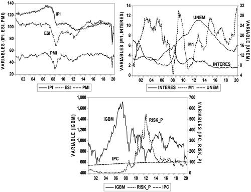
Table 1. Variables, statistical description.

Statistics	IGBM	INTERES	IPI	CPI	M1	PMI	UNEM	ESI	RISK_P
Mean	994.82	3.02	111.54	92.99	7.67	49.77	15.98	98.81	105.89
Median	955.44	2.99	105.70	95.56	7.95	51.04	15.30	103.50	76.90
Maximum	1.724.4	7.07	136.75	105.30	14.5	57.17	26.3	111.4	547.7
Minimum	576.20	1.5	70.58	71.94	0.28	28.49	7.90	68.7	0.50
Std. Dev.	237.32	1.44	13.30	9.79	3.09	5.11	5.69	9.97	116.42
Skewness	1.03	0.80	0.25	−0.61	−0.31	−1.64	0.28	−1.02	1.61
Kurtosis	4.05	2.81	2.01	2.07	2.54	6.52	1.79	3.20	5.43
Jarque-Bera	54.05	26.08	12.20	23.94	6.04	232.70	17.71	42.33	163.06
Probability	0.00	0.00	0.00	0.00	0.04	0.00	0.00	0.00	0.00

Source: own elaboration.

In general, the variables do not conform to a normal distribution and fluctuate over a relatively wide range, with periods of strong instability. As a consequence, their temporal behaviours and variability reflect non-stationarity and require a logarithmic transformation to reduce dispersion (represented by initial ‘L’).

4.2. Var/VECM model estimation

The estimation of the model is carried out with the endogenous variables transformed into logarithms. The next stage in the estimation process of the VAR/VECM model requires analyzing the stationarity and the possibility of cointegration of these variables.

The stationarity analysis is performed with the Dickey-Fuller Augmented and Philips- Perron tests without exogenous variable, testing for the existence of unit roots for each series in level and in first differences. In general, the null hypothesis (H₀: unit root exists) for the ‘series in level’ is not rejected, indicating the lack of stationarity, while the null hypothesis for the ‘series in first differences’ is rejected, so that the series are integrable of order 1, I (1) (Table 2).

Table 2. Unit root test, in levels and 1st difference.

Series		Level		1^st difference
Variables		Dickey-Fuller Augmented	Philips-Perron	Dickey-Fuller Augmented	Philips-Perron
LIGBM	t-statistic	−0.26	−0.26	−5.62	−14.54
	p-value	0.59	0.59	0.00	0.00
LINTERES	t-statistic	−1.77	−1.99	−2.84	−10.80
	p-value	0.08	0.05	0.00	0.00
LIPI	t-statistic	−0.51	−0.63	−13.46	−13.94
	p-value	0.49	0.44	0.00	0.00
LIPC	t-statistic	1,31	−3.61	−1,92	−18.21
	p-value	0.95	0.99	0.05	0.00
LM1	t-statistic	−0.22	−0.38	−4.92	−12.23
	p-value	0.60	0.54	0.00	0.00
LPMI	t-statistic	−0.01	−0.07	−13.23	−13.11
	p-value	0.68	0.65	0.00	0.00
LUNEM	t-statistic	0.18	0.43	−2.87	−6.12
	p-value	0.73	0.80	0.00	0.00
LESI	t-statistic	−0.55	−0.55	−4.58	−15.19
	p-value	0.47	0.47	0.00	0.00
LRISK_P	t-statistic	−0.59	−1.01	−23.72	−27.22
	p-value	0.46	0.27	0.00	0.00

Source: own elaboration.

On the other hand, to study the cointegration of the variables, a regression model is estimated and the existence of unit roots in the residuals is tested (Granger, 1986). The application of the Augmented Dickey-Fuller and Philips-Perron tests reflects the lack of stationarity and the non-cointegration of the variables, since the null hypothesis is not rejected (Table 3).

Table 3. Regression model and residuals test.

Dependent Variable: LIGBM					RESIDUALS
Variable	Coefficient	Std. Error	t-Statistic	Prob.
LINTERES	0.285	0.056	5.032	0.000	Null Hypothesis: RESIDUALS has a unit root (Exogenous: Constant)		t-Statistic	Prob.
LIPI	−0.231	0.205	−1.122	0.262
LIPC	1.677	0.155	10.823	0.000
LM1	−0.057	0.024	−2.344	0.019
LPMI	1.299	0.162	7.993	0.000	Augmented Dickey-Fuller		−2.526	0.110
LUNEM	−0.396	0.065	−6.093	0.000	Test critical values:	1% level	−3.457
LESI	−0.822	0.168	−4.886	0.000		5% level	−2.873
LRISK_P	−0.014	0.013	−1.085	0.278		10% level	−2.573

Source: own elaboration.

Therefore, the lack of cointegration of the variables leads to choosing a VAR model, although it is necessary to convert the series into stationary variables through differencing (represented with initial ‘D’).

Another step in the development of a VAR model is to define the optimal lags number. Many lags unnecessarily reduce the freedom degrees and few lags lead to misspecification, which influences the residuals autocorrelation. Different criteria are applied to select the optimal lag length; the results are: Schwarz (SC) and Hannan-Quinn (HQ) obtain one lag; Akaike (AIC) and Sequential test (LR) obtain six lags. The choice between these alternatives also requires the absence of autocorrelation in the residuals; this property is only verified with six lags, then the model defined corresponds to a VAR (6) (Table 4).

Table 4. Lag selection VAR model (*Lag chosen by criterion, 5% level).

Lag	LogL	LR	AIC	SC	HQ
1	3812.41	NA	−32.30	−31.09*	−31.81*
2	3919.76	197.97	−32.53	−30.12	−31.56
3	4019.36	175.90	−32.69	−29.07	−31.23
4	4106.34	146.85	−32.74	−27.91	−30.80
5	4202.99	155.64	−32.88	−26.84	−30.44
6	4308.48	161.66*	−33.09*	−25.85	−30.17
7	4358.46	72.69	−32.82	−24.37	−29.41
8	4430.91	99.73	−32.75	−23.09	−28.85

Source: own elaboration.

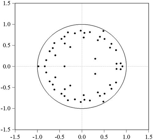
Next, it is also relevant to study the model stability; this condition depends on the roots value of the characteristic polynomial. In this analysis, all roots are less than one and this verifies the stationarity condition (Figure 2).

Figure 2. Inverse roots of the characteristic polynomial AR.

Source: own elaboration.

On the other hand, the temporal relationship between the variables means the existence of causality and establishes the direction of the information transmission. For this purpose, the Granger test is applied for pairs of variables and for six lags (Table 5).

Table 5. Granger causality between variables (lags: 6).

	Null Hypothesis (doesn’t Cause)	Prob.		Null Hypothesis (doesn’t Cause)	Prob.
D(LIGBM)	D(LINTERES) on D(LIGBM)	0.005	D(LIPI)	D(LIPC) on D(LIPI)	0.200
	D(LIGBM) on D(LINTERES)	0.049		D(LIPI) on D(LIPC)	0.697
	D(LIPI) on D(LIGBM)	0.110		D(LM1) on D(LIPI)	0.192
	D(LIGBM) on D(LIPI)	0.010		D(LIPI) on D(LM1)	0.596
	D(LIPC) on D(LIGBM)	0.455		D(LPMI) on D(LIPI)	0.165
	D(LIGBM) on D(LIPC)	0.099		D(LIPI) on D(LPMI)	0.001
	D(LM1) on D(LIGBM)	0.010		D(LUNEM) on D(LIPI)	0.000
	D(LIGBM) on D(LM1)	0.145		D(LIPI) on D(LUNEM)	0.000
	D(LPMI) on D(LIGBM)	0.004		D(LESI) on D(LIPI)	0.060
	D(LIGBM) on D(LPMI)	0.000		D(LIPI) on D(LESI)	0.000
	D(LUNEM) on D(LIGBM)	0.013		D(LRISK_P) on D(LIPI)	0.384
	D(LIGBM) on D(LUNEM)	0.060		D(LIPI) on D(LRISK_P)	0.279
	D(LESI) on D(LIGBM)	0.177	D(LIPC)	D(LM1) on D(LIPC)	0.185
	D(LIGBM) on D(LESI)	0.000		D(LIPC) on D(LM1)	0.029
	D(LRISK_P) on D(LIGBM)	0.943		D(LPMI) on D(LIPC)	0.182
	D(LIGBM) on D(LRISK_P)	0.845		D(LIPC) on D(LPMI)	0.003
D(LINTERES)	D(LIPI) on D(LINTERES)	0.455		D(LUNEM) on D(LIPC)	0.094
	D(LINTERES) on D(LIPI)	0.626		D(LIPC) on D(LUNEM)	0.875
	D(LIPC) on D(LINTERES)	0.001		D(LESI) on D(LIPC)	0.716
	D(LINTERES) on D(LIPC)	0.030		D(LIPC) on D(LESI)	0.143
	D(LM1) on D(LINTERES)	0.000		D(LRISK_P) on D(LIPC)	0.799
	D(LINTERES) on D(LM1)	0.384		D(LIPC) on D(LRISK_P)	0.909
	D(LPMI) on D(LINTERES)	0.563	D(LM1)	D(LPMI) on D(LM1)	0.938
	D(LINTERES) on D(LPMI)	0.023		D(LM1) on D(LPMI)	0.000
	D(LUNEM) on D(LINTERES)	0.172		D(LUNEM) on D(LM1)	0.719
	D(LINTERES) on D(LUNEM)	0.041		D(LM1) on D(LUNEM)	0.020
	D(LESI) on D(LINTERES)	0.615		D(LESI) on D(LM1)	0.813
	D(LINTERES) on D(LESI)	0.087		D(LM1) on D(LESI)	0.040
	D(LRISK_P) on D(LINTERES)	0.997		D(LRISK_P) on D(LM1)	0.561
	D(LINTERES) on D(LRISK_P)	0.642		D(LM1) on D(LRISK_P)	0.234
D(LUNEM)	D(LESI) on D(LUNEM)	0.000	D(LPMI)	D(LUNEM) on D(LPMI)	0.000
	D(LUNEM) on D(LESI)	0.000		D(LPMI) on D(LUNEM)	0.000
	D(LRISK_P) on D(LUNEM)	0.453		D(LESI) on D(LPMI)	0.019
	D(LUNEM) on D(LRISK_P)	0.037		D(LPMI) on D(LESI)	0.000
D(LESI)	D(LRISK_P) on D(LESI)	0.128		D(LRISK_P) on D(LPMI)	0.441
	D(LESI) on D(LRISK_P)	0.834		D(LPMI) on D(LRISK_P)	0.868

Source: own elaboration.

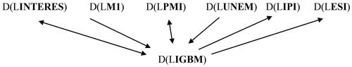
This causality analysis confirms the interaction between some macroeconomic variables and the stock market. This relationship can be unidirectional or bidirectional, so single or double arrows are used in the figures for their representation. More specifically, the macroeconomic variables corresponding to the interest rate, the monetary aggregate M1, the manufacturing activity index and the unemployment rate (D(LINTERES), D(LM1), D(LPMI), D(LUNEM)) affect the stock market D(LIGBM). Likewise, the stock market D(LIGBM) influences some macroeconomic variables, such as the interest rate and industrial production, manufacturing activity and economic sentiment indices (D(LINTERES), D(LIPI), D(LPMI), D(LESI)) (Figure 3).

Figure 3. Causality between macroeconomic variables and the stock market.

Source: own elaboration.

The existence of a causal relationship between the different macroeconomic variables is also verified for the monetary variables (interest rate, inflation and monetary aggregate M1) and for the activity variables (D(LIPI), D(LPMI), D(LESI), D(LUNEM)). The monetary variables, the interest rate D(LINTERES) and inflation D(LIPC) have a mutual relationship; they also have an indirect effect through the monetary aggregate M1 D(LM1) (Figure 4).

Figure 4. Causality between macroeconomic variables.

(Interest, Inflation, Monetary Aggregate M1)

Source: own elaboration.

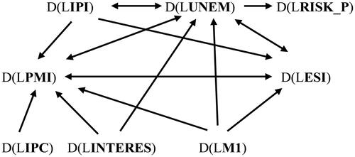
Similarly, there is a bidirectional causal relationship between the activity indices (industrial production D(LIPI), manufacturing activity D(LPMI), economic sentiment D(LESI)) and the unemployment rate D(LUNEM). In addition, most of these variables are influenced by monetary variables (interest rate D(LINTERES), inflation D(LIPC) and monetary aggregate M1 D(LM1)). The unemployment rate D(LUNEM) is also found to have an influence on the risk premium D(LRISK_P) (Figure 5).

Figure 5. Causality between macroeconomic variables.

(Interest rate, Inflation, Activity indices, Monetary aggregate M1, Risk premium)

Source: own elaboration.

The estimation of the VAR (6) model makes it necessary to test its validity through the analysis of the residuals, with the study of autocorrelation, normality and homoscedasticity. To test for autocorrelation, the Lagrange test (maximum likelihood) is used, the null hypothesis of the existence of autocorrelation being rejected. To study the normality of the residuals, Cholesky orthogonalization is performed and the Jarque-Bera test is used, which rejects the null hypothesis of normal distribution of the residuals, but some authors point out that this lack of normality does not affect the validity of the model (Lanne & Lütkepohl, 2010; Gonzalo, 1994; among others). Finally, to verify homoscedasticity in the residuals, the White test is applied without cross-terms, whose null hypothesis of homoscedasticity in the variance is not rejected.

Verification of the validity of the VAR (6) model allows analyses such as the study of the ‘Impulse-Response Function’, a procedure that addresses the temporary effect that an impulse or modification in each of the variables would produce on the rest of the variables. Thus, an impact on a variable not only affects the variable itself, but is also transmitted dynamically to the other variables owing to its interrelationship.

In order to analyze the responses of each variable to the different shocks, the following differentiation is made: the response of each variable to its own shocks, the interrelation of macroeconomic variables and the stock market, and the relationship between macroeconomic variables. These analysis are dealt with at a theoretical level, however, due to the limited graphical visualisation, only the impulse-response of macroeconomic variables and stock market are shown.

• The response of each variable to its own shocks is generally decreasing and is damped over time until it virtually disappears, although this is not the case for the unemployment rate and the inflation rate, whose responses to their own shocks tend to be sustained over time.

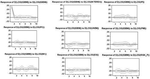
• The relationship between macroeconomic variables and the stock market is established in both directions. However, not all macroeconomic variables have a significant impact on the stock market index; only the monetary aggregate M1 D(LM1) has a positive impact on the stock market D(LIGBM) and the interest rate D(LINTERES) and the unemployment rate D(LUNEM) have a negative effect (Figure 6).

Figure 6. Impulse-response function (One S.D. Innovations ± 2 S.E.).

Stock market D(LIGBM) response to impacts the macroeconomic variables

Source: own elaboration.

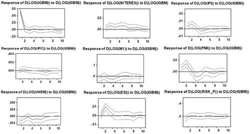
There is also an impact of the stock market D(LIGBM) on macroeconomic variables, with a positive impact on the interest rate D(LINTERES) and on the indices of industrial production, manufacturing activity and economic sentiment (D(LIPI), D(LPMI), D(LESI)) and a negative impact on the unemployment rate (D(LUNEM)) (Figure 7).

Figure 7. Impulse-response function (One S.D. Innovations ± 2 S.E.).

Macroeconomic variables response to impacts the stock market D(LIGBM)

Source: own elaboration.

• • The relationship between the set of macroeconomic variables identifies the effects that any changes have on the real economy itself. However, this relationship will depend on the response variable and the different impacts, so it is important to analyse the different interrelationships.

•   ^ The response of the interest rate D(LINTERES) is significant for shocks corresponding to the monetary aggregate D(LM1) and the inflation rate D(LIPC) with the opposite impact, negative for the monetary aggregate and positive for the inflation rate. Likewise, inflation D(LIPC) has a negative impact on the monetary aggregate M1 D(LM1).

•   ^ The response of the industrial production index D(LIPI) is only relevant to the impact of the unemployment rate D(LUNEM) with a negative effect. In addition, the unemployment rate (D(LUNEM)) have a positive impact on the risk premium D(LRISK_P). On the contrary, the response of the unemployment rate D(LUNEM) is negative to the impact of the industrial production index D(LIPI) and the monetary aggregate M1 D(LM1).

•   ^ The response of the manufacturing activity index and the economic sentiment index (D(LPMI), D(LESI)) is generally similar to different shocks. The index of manufacturing activity D(LPMI) evolves positively to the industrial production index and the monetary aggregate M1 (D(LIPI), D(LM1)) and negatively to the interest rate, inflation and the unemployment rate (D(LINTERES), D(LIPC), D(LUNEM)). Also, the economic sentiment index D(LESI) reacts positively to the impact of the industrial production index, the manufacturing activity index and the monetary aggregate M1 (D(LIPI)), D(LPMI), D(LM1)) and negatively to the unemployment rate D(LUNEM).

5. Discussion

The aim of this paper has been to analyze the interrelationship between the financial stock market and the macroeconomic environment in Spain and, from a general point of view, the results obtained confirm the existence of a relationship, coinciding with other researchers (Abdelbaki, 2013; Alam & Uddin, 2009; Ali & Chowdhury, 2021; Farsio & Fazel, 2013; Fromentin et al., 2022). However, this general conclusion leads to analyze the behaviour of each variable by identifying its significance and effect on the stock market and to contrast these results with those obtained in other studies.

In relation to the interest rate and inflation, they have traditionally been considered to have a negative relationship on the stock market, with the result that lower interest rates have a positive influence on the stock market (Alam & Uddin, 2009; Engsted & Tanggaard, 2002; Fama, 1981; Gjerde & Sættem, 1999; Omran, 2003; Wongbangpo & Sharma, 2002). This behaviour of the interest rate is quite widespread; this is not so for inflation, where there is research questioning this relationship as not significant (Buyuksalvarci 2010; Ilahi et al., 2015; Imdadullah & Hayatabad, 2012; Subeniotis et al., 2011; Uwubanmwen & Eghosa, 2015). In this paper, the interest rate negatively influences the stock market in a somewhat lagged manner, but also the stock market positively affects the interest rate. However, inflation does not have any impact. The behaviour of the interest rate is consistent with other research, while in the case of inflation the result obtained corresponds to those pointing to the lack of relationship.

As for the money supply or monetary aggregate M1, generally, researchers relate its positive growth to the stock market, since when inflation is controlled as it is in Spain, an increase in the money supply usually leads to reductions in the interest rate, positively affecting economic activity (Abdelbaki, 2013; Asriyan et al., 2021; Gan et al., 2006; Maysami & Koh, 2000). In this research, the impact of the monetary aggregate M1 has a positive and lagged influence on the financial market in line with the literature.

The industrial production index, the economic sentiment index and the manufacturing sector activity index are three indicators that reflect the situation or perception of economic and business activity. There are no clear criteria in the literature on the behaviour of these variables on the stock market. Thus, in the case of the industrial production index, there are different opinions, with some authors expressing the existence of a positive impact (Flannery & Protopapadakis, 2002; Humpe & Macmillan, 2009; Liu & Shrestha, 2008; Shanken & Weinstein, 2006; Thalassinos et al., 2006), while others point out that its impact is inconclusive (Fama, 1981; Gultekin, 1983; Subeniotis et al., 2011). There is also no consensus on the impact of the economic sentiment index on the stock market, some researchers relating it positively (Baker & Wurgler, 2006; Estrella & Hardouvelis, 1991; Estrella & Mishkin, 1997; Hüfner & Schröder, 2002; Subeniotis et al., 2011), although there is also research that points to their lack of relationship (Ho & Hung, 2012). Likewise, the behaviour of the manufacturing activity index is not conclusive; there are authors who indicate a positive relationship with the stock market (Afshar et al., 2007; Alsu & Mandaci, 2020; Baum et al., 2015; Hüfner and Schröder 2002; Johnson & Watson, 2011; Kvietkauskienė & Plakys, 2017; Lupu, 2018), while others differ (Akdağ et al. 2020; Yanik et al., 2020) or some, such as Vieira et al. (2013), indicate the negative influence of this variable on the stock market.

In this research, the industrial production index and the economic sentiment index do not have a relevant impact on the stock market, but the manufacturing activity index has a positive effect.

Regarding the unemployment rate having a negative effect on the stock market (Boyd et al., 2005; Farsio & Fazel, 2013, Tapa et al., 2016; Sirucek, 2012), in this study, the unemployment rate also has a negative impact, coinciding with the general opinion of other authors.

As for the risk premium, there are no clear criteria about its influence, and there are discrepancies about its repercussions on the stock market (Aristei & Martelli, 2014; Augustin et al., 2018; Bernoth et al., 2012; Chiu & Lee, 2019; Chovancová et al., 2019; Haugh et al., 2009; Pierdzioch et al., 2008; Silvapulle et al., 2016; Singh et al., 2011). However, this variable has been controlled by the European Central Bank in the case of Spain and other EU countries; the European Central Bank’s decision to intervene since the 2008 crisis in secondary debt markets has led to a reduction in the Spanish risk premium, from peak values close to 550 points in 2012 to levels close to 100 points in 2021. Therefore, this situation of intervention and relative control of the risk premium has limited its movements, which may be one of the reasons why this variable has no influence on the stock market in this research work.

6. Conclusions

This article analyzes the transmission of effects between the macroeconomic environment and the stock market in Spain, using a VAR model for the period 2001–2020. The selection of this study period is relevant for the analysis as it allows us to include the information corresponding to the major crises that have occurred in this century (financial 2008 and health 2019).

The main contributions obtained can be grouped as follows:

• • Stock market response to impacts the macroeconomic variables:

•   ^ Positive effect: monetary aggregate M1 and lagged manufacturing activity index (PMI).

•   ^ Negative effect: unemployment rate (UNEM) and lagged interest rate (INTERES).

• • Macroeconomic variables response to impacts the stock market:

•   ^ Positive impact: interest rate (INTERES), industrial production index (IPI), manufacturing activity index (PMI) and economic sentiment index (ESI).

•   ^ Negative impact: unemployment rate (UNEM).

The relationship between macroeconomic variables is also confirmed, although the effect depends on the variable. Therefore, changes in the real economy also have an impact on the economy itself.

In short, this research has practical implications for the Public Administration by allowing possible risks to be detected in the real and financial economy, and for investors, who have the possibility of deciding their investments with the information of the market itself and with some macroeconomic variables, knowing their incidence on the stock market.

This study has certain limitations:

• The data analyzed are only from Spain and correspond to an extensive but limited period.

• There may be other macroeconomic variables that could have an influence on the stock market or other international variables influencing the Spanish stock market that were not considered in the study.

Future lines of research could be developed further in this area of study, either by extending the time horizon, analyzing other countries, using alternative approaches or incorporating new variables.

Disclosure statement

No potential conflict of interest was reported by the authors.

References

- Abdelbaki, H. (2013). Causality relationship between macroeconomic variables and stock market development: Evidence from Bahrain. The International Journal of Business and Finance Research, 7(1), 69–84.
- Afshar, T., Arabian, G., & Zomorrodian, R. (2007). Stock return, consumer confidence, purchasing managers index and economic fluctuations. Journal of Business & Economics Research, 5(8), 97–106.
- Alam, M., & Uddin, M. (2009). Relationship between interest rate and stock price: Empirical evidence from developed and developing countries. International Journal of Business and Management, 4(3), 43–51. https://doi.org/10.5539/ijbm.v4n3p43
- Ali, I., Rehman, K., Yilmaz, A., Khan, M., & Afzal, H. (2010). Causal relationship between macroeconomic indicators and stock exchange prices in Pakistan. African Journal of Business Management, 4(3), 312–319.
- Ali, M., & Chowdhury, M. A. A. (2021). Dynamic interaction between conditional stock market volatility and macroeconomic uncertainty of Bangladesh. Asian Journal of Business Environment, 11(4), 17–29.
- Alsu, E., & Mandaci, P. E. (2020). Is purchasing managers’index (PMI) a leading indicator for stock, bond and foreign exchange markets in Turkey. İşletme Fakültesi Dergisi, 21(1), 219–233. https://doi.org/10.24889/ifede.605338
- Aristei, D., & Martelli, D. (2014). Sovereign bond yield spreads and market sentiment and expectations: Empirical evidence from Euro area countries. Journal of Economics and Business, 76, 55–84. https://doi.org/10.1016/j.jeconbus.2014.08.001
- Asriyan, V., Fornaro, L., Martin, A., & Ventura, J. (2021). Monetary policy for a bubbly world. The Review of Economic Studies, 88(3), 1418–1456. https://doi.org/10.1093/restud/rdaa045
- Ato, J., & Janrattanagul, J. (2014). Selected macroeconomic variables and stock market movements: Empirical evidence from Thailand. Contemporary Economics, 8(2), 157–174. https://doi.org/10.5709/ce.1897-9254.138
- Augustin, P., Boustanifar, H., Breckenfelder, J., & Schnitzler, J. (2018). Sovereign to corporate risk spillovers. Journal of Money, Credit and Banking, 50(5), 857–891. https://doi.org/10.1111/jmcb.12497
- Baker, M., & Wurgler, J. (2006). Investor sentiment and the cross-section of stock returns. The Journal of Finance, 61(4), 1645–1680. https://doi.org/10.1111/j.1540-6261.2006.00885.x
- Balke, N., & Wohar, M. (2001). Explaining Stock price movements: Is there a case for fundamentals? Economic and Financial Review-Federal Reserve Bank of Dallas, (3), 22–33.
- Baum, C., Kurov, A., & Wolfe, M. (2015). What do Chinese macro announcements tell us about the world economy? Journal of International Money and Finance, 59, 100–122. https://doi.org/10.1016/j.jimonfin.2015.07.002
- Bernoth, K., Hagen, J., & Schuknecht, L. (2012). Sovereign risk premiums in the European government bond markets. Journal of International Money and Finance, 31(5), 975–995. https://doi.org/10.1016/j.jimonfin.2011.12.006
- Boyd, J., Hu, J., & Jagannathan, R. (2005). The stock market’s reaction to unemployment news: ‘Why bad news is usually good for stocks. The Journal of Finance, 60(2), 649–672. https://doi.org/10.1111/j.1540-6261.2005.00742.x
- Büyükşalvarcı, A. (2010). The effects of macroeconomics variables on stock returns: Evidence from Turkey. European Journal of Social Science, 14(3), 404–416.
- Chen, N. F., Roll, R., & Ross, S. A. (1986). Economic forces and the stock market. The Journal of Business, 59(3), 383–403. https://doi.org/10.1086/296344
- Cheung, Y., & Ng, K. (1998). International evidence on the stock market and aggregate economic activity. Journal of Empirical Finance, 5(3), 281–296. https://doi.org/10.1016/S0927-5398(97)00025-X
- Chiu, Y., & Lee, C. (2019). Financial development, income inequality, and country risk. Journal of International Money and Finance, 93, 1–18. https://doi.org/10.1016/j.jimonfin.2019.01.001
- Chovancová, B., Árendáš, P., Slobodník, P., & Vozňáková, I. (2019). Country risk at investing in capital markets – The case of Italy. Problems and Perspectives in Management, 17(2), 440–448. https://doi.org/10.21511/ppm.17(2).2019.34
- Cooper, R., Chuin, L., & Atkin, M. (2004). Relationship between macroeconomic variables and stock market indices: Cointegration evidence from stock exchange of Singapore’s All-S sector indices. Journal Pengurusan, 24, 47–77.
- European Central Bank. ( 2020). Dataset, annual interest rate for house purchases (Spain) and the monetary aggregate M1 in the EU. 2001-2020. Retrieved June 26, 2021, from https://sdw.ecb.europa.eu
- Engsted, T., & Tanggaard, C. (2002). The relation between asset returns and inflation at short and long horizons. Journal of International Financial Markets, Institutions and Money, 12(2), 101–118. https://doi.org/10.1016/S1042-4431(01)00052-X
- Estrella, A., & Hardouvelis, G. (1991). The term structure as a predictor of real economic activity. The Journal of Finance, 46(2), 555–576. https://doi.org/10.1111/j.1540-6261.1991.tb02674.x
- Estrella, A., & Mishkin, F. (1997). The term structure of interest rates and its role in monetary policy for the European Central Bank. European Economic Review, 41(7), 1375–1401. https://doi.org/10.1016/S0014-2921(96)00050-5
- Estrella, A., & Mishkin, F. (1998). Predicting U.S. recessions: Financial variables as leading indicators. Review of Economics and Statistics, 80(1), 45–61. https://doi.org/10.1162/003465398557320
- Eurostat. (2020). Dataset, economic sentiment index 2001-2020. Retrieved June 26, 2021, https://ec.europa.eu/eurostat/data/database
- Expansión. (2020). Dataset, unemployment rate 2001-2020. Retrieved June 26, 2021, from https://datosmacro.expansion.com
- Fama, E. (1970). Efficient capital markets: A review of theory and empirical work. The Journal of Finance, 25(2), 383–417. https://doi.org/10.2307/2325486
- Fama, E. (1981). Stock returns, real activity, inflation, and money. American Economic Review, 71(4), 545–565.
- Fama, E. (1990). Stock returns expected returns and real activity. The Journal of Finance, 45(4), 1089–1108. https://doi.org/10.1111/j.1540-6261.1990.tb02428.x
- Farsio, F., & Fazel, S. (2013). The stock market/unemployment relationship in USA, China and Japan. International Journal of Economics and Finance, 5(3), 24–29. https://doi.org/10.5539/ijef.v5n3p24
- Fisher, I. (1920). The purchasing power of money: Its determination and relation to credit interest and crises. Macmillan Company.
- Flannery, M., & Protopapadakis, A. (2002). Macroeconomic factors do influence aggregate stock returns. Review of Financial Studies, 15(3), 751–782. https://doi.org/10.1093/rfs/15.3.751
- Fromentin, V., Lorraine, M. S. H., Ariane, C., & Alshammari, T. (2022). Time-varying causality between stock prices and macroeconomic fundamentals: Connection or disconnection? Finance Research Letters, 49, 103073. https://doi.org/10.1016/j.frl.2022.103073
- Gan, C., Lee, M., Au Yong, H. H., & Zhang, J. (2006). Macroeconomic variables and stock market interactions: New Zealand evidence. Investment Management and Financial Innovations, 3(4), 89–101.
- Giri, A. K., & Pooja, J. (2017). The impact of macroeconomic indicators on Indian stock prices: An empirical analysis. Studies in Business and Economics, 12(1), 61–78. https://doi.org/10.1515/sbe-2017-0005
- Gjerde, Ø., & Sættem, F. (1999). Causal relations among stock returns and macroeconomic variables in a small, open economy. Journal of International Financial Markets, Institutions and Money, 9(1), 61–74. https://doi.org/10.1016/S1042-4431(98)00036-5
- Gonzalo, J. (1994). Five alternative methods of estimating long-run equilibrium relationships. Journal of Econometrics, 60(1-2), 203–233. https://doi.org/10.1016/0304-4076(94)90044-2
- Granger, C. (1986). Developments in the study of co integrated economic variables, Oxford. Oxford Bulletin of Economics and Statistics, 48(3), 213–228. https://doi.org/10.1111/j.1468-0084.1986.mp48003002.x
- Gultekin, N. (1983). Stock market returns and inflation: Evidence from other countries. The Journal of Finance, 38(1), 49–65. https://doi.org/10.1111/j.1540-6261.1983.tb03625.x
- Haugh, D., Olluvaud, P., & Turner, D. (2009). What drives sovereign risk premiums? An analysis of recent evidence from the euro area. OECD Economics Department Working Papers No. 718, 1–24. https://doi.org/10.1787/222675756166
- Ho, J., & Hung, C. (2012). Predicting stock market returns and volatility with investor sentiment: Evidence from eight developed countries. Journal of Accounting and Finance, 12(4), 49–65.
- Hüfner, F. P., & Schröder, M. (2002). Forecasting economic activity in Germany – How useful are sentiment indicators? ZEW. Center for European Economic Research, No. 02-56, 1–14. https://doi.org/10.2139/ssrn.339141
- Humpe, A., & Macmillan, P. (2009). Can macroeconomic variables explain long-term stock market movements? A comparison of the US and Japan. Applied Financial Economics, 19(2), 111–119. https://doi.org/10.1080/09603100701748956
- Ikoku, A. (2010). Is the stock market a leading indicator of economic activity in Nigeria? Journal of Applied Statistics, 1(1), 17–38.
- Ilahi, I., Ali, M., & Jamil, R. (2015). Impact of macroeconomic variables on stock market returns: A case of Karachi stock exchange. No. 2016-03. https://doi.org/10.2139/ssrn.2583401
- IMF. (2020). Global Financial Stability Report Update. International Monetary Fund.
- Imdadullah, M. B. A., & Hayatabad, P. (2012). Impact of interest rate, exchange rate and inflation on stock returns of KSE 100 index. International Journal Economic, 3(5), 142–155.
- Investing. (2020). Dataset, general index of the Madrid Stock Exchange, manufacturing sector activity (PMI) and Spain’s risk premium 2001-2020. Retrieved June 26, 2021, from https://es.investing.com
- Jansen, W., & Nahuis, N. (2003). The stock market and consumer confidence: European evidence. Economics Letters, 79(1), 89–98. https://doi.org/10.1016/S0165-1765(02)00292-6
- Johnson, M., & Watson, K. (2011). Can changes in the purchasing managers’ index foretell stock returns? An additional forward-looking sentiment indicator. The Journal of Investing, 20(4), 89–98. https://doi.org/10.3905/joi.2011.2011.1.016
- Kvietkauskienė, A., & Plakys, M. (2017). Impact indicators for stock markets return. Poslovna izvrsnost - Business Excellence, 11(2), 59–83. https://doi.org/10.22598/pi-be/2017.11.2.59
- Lanne, M., & Lütkepohl, H. (2010). Structural vector autoregressions with nonnormal residuals. Journal of Business & Economic Statistics, 28(1), 159–168. https://doi.org/10.1198/jbes.2009.06003
- Liu, M., & Shrestha, K. (2008). Analysis of the long-term relationship between macro- economic variables and the Chinese stock market using heteroscedastic cointegration. Managerial Finance, 34(11), 744–755. https://doi.org/10.1108/03074350810900479
- Lupu, I. (2018). Analysis of how the European stock markets perceive the dynamics of macroeconomic indicators through the sentiment index and the purchasing managers’ index. Financial Studies, 22(1(79), 32–52.
- Maio, P., & Philip, D. (2015). Macro variables and the components of stock returns. Journal of Empirical Finance, 33, 287–308. https://doi.org/10.1016/j.jempfin.2015.03.004
- Maysami, R., & Koh, T. (2000). A vector error correction model of the Singapore stock market. International Review of Economics & Finance, 9(1), 79–96. https://doi.org/10.1016/S1059-0560(99)00042-8
- Mukherjee, T. K., & Naka, A. (1995). Dynamic relations between macroeconomic variables and the Japanese stock market: An application of a vector error correction model. Journal of Financial Research, 18(2), 223–237. https://doi.org/10.1111/j.1475-6803.1995.tb00563.x
- National Statistics Institute. (2020). Dataset, industrial production and consumer price indices 2001-2020. Retrieved June 26, 2021, from https://www.ine.es
- Nasseh, A., & Strauss, J. (2000). Stock prices and domestic and international macroeconomic activity: A cointegration approach. The Quarterly Review of Economics and Finance, 40(2), 229–245. https://doi.org/10.1016/S1062-9769(99)00054-X
- Nishat, M., Shaheen, R., & Hijazi, S. T. (2004). Macroeconomic factors and the Pakistani equity market. The Pakistan Development Review, 43(4II), 619–637. http://www.jstor.org/stable/41261017 https://doi.org/10.30541/v43i4IIpp.619-637
- Okun, A. (1962). Potential GNP: Its Measurement and Significance. In Proceedings of the Business and Economic Statistics Section of the American Statistical Association (pp. 89–104). American Statistical Association.
- Omran, M. (2003). Time series analysis of the impact of real interest rates on stock market activity and liquidity in Egypt: Co-integration and error correction model approach. International Journal of Business, 8(3), 359–374.
- Pal, K., & Mittal, R. (2011). Impact of macroeconomic indicators on Indian capital markets. The Journal of Risk Finance, 12(2), 84–97. https://doi.org/10.1108/15265941111112811
- Phillips, A. (1958). The relation between unemployment and the rate of change of money wages in the United Kingdom 1861–1957. Economica, 25(100), 283–299. https://doi.org/10.1111/j.1468-0335.1958.tb00003.x
- Pierdzioch, C., Döpke, J., & Hartmann, D. (2008). Forecasting stock market volatility with macroeconomic variables in real time. Journal of Economics and Business, 60(3), 256–276. https://doi.org/10.1016/j.jeconbus.2007.03.001
- Pilinkus, D., & Boguslauskas, V. (2009). The short-run relationship between stock market prices and macroeconomic variables in Lithuania: An application of the impulse response function. Inzinerine Ekonomika-Engineering Economics, 66, 1–9.
- Ratanapakorn, O., & Sharma, S. (2007). Dynamics analysis between the US stock return and the macroeconomics variables. Applied Financial Economics, 17(5), 369–377. https://doi.org/10.1080/09603100600638944
- Rjoub, H., Türsoy, T., & Günsel, N. (2009). The effects of macroeconomic factors on stock returns: Istanbul Stock Market. Studies in Economics and Finance, 26(1), 36–45. https://doi.org/10.1108/10867370910946315
- Schwert, G. (1990). Stock returns and real activity: A century of evidence. The Journal of Finance, 45(4), 1237–1257. https://doi.org/10.1111/j.1540-6261.1990.tb02434.x
- Shanken, J., & Weinstein, M. (2006). Economic forces and the stock market revisited. Journal of Empirical Finance, 13(2), 129–144. https://doi.org/10.1016/j.jempfin.2005.09.001
- Silvapulle, P., Fenech, J. P., Thomas, A., & Brooks, R. (2016). Determinants of sovereign bond yield spreads and contagion in the peripheral EU countries. Economic Modelling, 58, 83–92. https://doi.org/10.1016/j.econmod.2016.05.015
- Singh, T., Mehta, S., & Varsha, M. (2011). Macroeconomic factors and stock returns: Evidence from Taiwan. Journal of Economics and International Finance, 2(4), 217–227.
- Sirucek, M. (2012). Macroeconomic variables and stock market: US review. International Journal of Computer Science and Management Studies, 12(3), 2231–5268.https://mpra.ub.uni-muenchen.de/39094/
- Subeniotis, D., Tampakoudis, I., Kroustalis, I., & Poülios, M. (2011). Empirical examination of wealth effect of mergers and acquisitions: The U.S. Economy in Perspective. Journal of Financial Management and Analysis, 24(2), 30–38.
- Tangjitprom, N. (2011). Macroeconomic factors of emerging stock market: The evidence from Thailand. SSRN Electronic Journal, 3(2), 105–114. https://doi.org/10.2139/ssrn.1957697
- Tapa, N., Tom, Z., Lekoma, M., Ebersohn, J., & Phiri, A. (2016). The unemployment-stock market relationship in South Africa: Evidence from symmetric and asymmetric cointegration models. MPRA Paper, 74101, 1–27. https://mpra.ub.uni-muenchen.de/74101/
- Thalassinos, E., Kyriazidis, T., & Thalassinos, J. (2006). The Greek capital market: Caught in between poor corporate governance and market inefficiency. European Research Studies Journal, IX(1-2), 3–24.
- Uwubanmwen, A., & Eghosa, I. (2015). Inflation rate and stock returns: Evidence from the Nigerian stock market. International Journal of Business and Social Science, 6(11), 155–167.
- Verma, R., & Ozuna, T. (2005). Are emerging equity markets responsive to cross-country macroeconomic movements? Evidence from Latin America. Journal of International Financial Markets, Institutions and Money, 15(1), 73–87. https://doi.org/10.1016/j.intfin.2004.02.003
- Vieira, E., Fernandes, C., & Gama, P. (2013). Market and macroeconomic fundamental dynamic interactions: ASEAN-5 countries. J. Asian Econ, 13, 27–51.
- Wongbangpo, P., & Sharma, S. (2002). Stock market and macroeconomic fundamental dynamic interactions: ASEAN-5 countries. Journal of Asian Economics, 13(1), 27–51. https://doi.org/10.1016/S1049-0078(01)00111-7
- Yanik, R., Binte, A., & Ozturk, O. (2020). Impact of manufacturing PMI on stock market index: A study on Turkey. Journal of Administrative and Business Studies, 6(3), 104–108. https://doi.org/10.20474/jabs-6.3.4