A new indicator of leaf stomatal conductance based on thermal imaging for field grown cowpea

ABSTRACT

Compared with a porometer, a thermal camera can be easily applied to large plant populations comprising a set of varieties, treatments, and replications, whereby, leaf temperature-based indicators are widely used to estimate stomatal conductance (g_s); however, a major difficulty in applying these indicators is their vulnerability to meteorological conditions. In this study, a new indicator of g_s (GsI) was developed with a modified theoretical equation of g_s that was highly simplified by means of several assumptions. GsI calculation uses leaf and air temperature, relative humidity, and solar radiation measurements. To validate and compare GsI values with other thermal indicators as leaf-air temperature difference and crop water stress index, glasshouse and field experiments were conducted. Leaf temperature of cowpea plants was measured using a low-cost thermal camera to ensure a cost-friendly method. GsI proved to be more stable than other indicators, relative to the measured g_s, irrespective of solar radiation, air temperature, and relative humidity conditions. As no reference temperature is needed for the calculation of GsI, it easily applies to large plant populations, although the GsI is most accurate in the range from moderate to high g_s values (approximately, >0.2 mol m⁻² s⁻¹). We used GsI to evaluate a cowpea germplasm collection consisting of 248 accessions, and elucidated that most accessions with higher GsI, which expected to have higher g_s, are originated in West-Africa. As GsI is available regardless of varying meteorological conditions, it is a useful indicator of g_s, especially in field studies involving multilocation and time-course evaluations.

Abbreviations: Cp: specific heat of the air; CWSI: crop water stress index; DAS: days after sowing; DT: saturated vapor pressure at temperature T; ea: vapor pressure of the air; es: vapor pressure at leaf surface; G: heat flux to the ground; ga: boundary layer conductance; gs: stomatal conductance; gv: total conductance; RH: relative humidity; Rn: net radiation; Rs: short-wave radiation; S: heat flux to the leaf; Ta: air temperature; Tdry: dry reference temperature; Ts: leaf surface temperature; Twet: wet reference temperature; VPD: vapor pressure deficit; γ: psychrometric constant; λE: latent heat flux; ρ: air density.

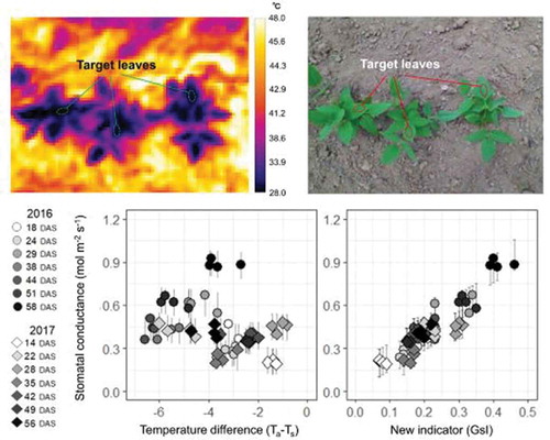
Graphical Abstract

KEYWORDS:

• Stomatal conductance
• thermal image
• cowpea
• gas exchange
• Bayesian analysis

1. Introduction

Stomatal conductance is a major regulator of water vapor and carbon dioxide exchange between the leaf and the surrounding air, which directly affects plant growth. Higher stomatal conductance or transpiration rates are well known to be closely related to better yield in several crop species, such as cotton, wheat, and rice (Fischer et al., 1997; Lu, Percy, Qualset & Zeiger, 1998; Takai, Yano & Yamamoto, 2010). Stomatal conductance also plays an important role in minimizing plant water loss to adapt to environments with varying levels of solar radiation, air humidity, air temperature, wind speed, and soil water content. Therefore, stomatal conductance is used as an indicator of plant water status and growth especially under mild-moderate drought stress conditions (Flexas & Medrano, 2002; Medrano et al., 2002).

Figure 5. Genetic variability for GsI among 248 accessions of cowpea genetic resources. GsI distributions at vegetative growth stage (a: 5 weeks after sowing) and at the beginning of maturity (b: 8 weeks after sowing). Distribution of the GsI values are separately shown for the three groups of cowpea accessions as per the classification by Fatokun et al. (2018), depending on genomic diversification.

The most accurate method to measure stomatal conductance is by using a leaf porometer or an infrared gas analyzer. Unfortunately, such devices are not suitable for frequent measurement within large plant populations because individual measurements take on average 20‒60 s per leaf. Additionally, the high cost of the instruments limits their availability to many low-budget experimental studies, and breeding programs. On the other hand, a recent improvement in genotyping technologies demands phenotypic information of large numbers of plants from cross-populations, breeding materials, and genetic resources. Remote-sensing technologies are available to meet this demand, and infrared thermal imaging is now widely used for the evaluation of stomatal conductance and transpiration rate at a scale varying from leaf to canopy (Costa, Grant & Chaves, 2013; Jones, 1999; Leinonen, Grant, Tagliavia, Chaves & Jones, 2006). Leaf surface and canopy temperatures can be easily determined by taking an infrared thermal image. Recently, the price of an infrared thermal camera has decreased, and an inexpensive model is available at less than 500 USD. To date, thermal imaging has been applied for evaluation not only of plant growth and drought stress, but also that of nutrient status and disease infection (Guo et al., 2016; Stoll, Schultz & Berkelmann-Loehnertz, 2008).

By using thermal imaging for leaf temperature determination, stomatal conductance can be theoretically calculated from variables including net radiation, air temperature, vapor pressure deficit, boundary layer resistance to water vapor, and parallel resistance to heat and radiative transfer (Jones, 2004). However, the complex equation is not user-friendly, and rigorous experiments are needed to give a precise estimate of resistance values (Brenner & Jarvis, 1995). As a simpler method, several indicators of stomatal conductance using thermal imaging have been developed, such as air-leaf temperature difference, crop water stress index (CWSI), stomatal conductance index (Ig), standard deviation of canopy temperature (CTSD), and canopy temperature difference (CTd) (Egea, Padilla-Diaz, Martinez-Guanter, Fernandez & Perez-Ruiz, 2017; Han, Zhang, DeJonge, Comas & Trout, 2016; Lima et al., 2016; Padhi, Misra & Payero, 2012; Takai et al., 2010). Because of the simplicity of evaluation and calculation, leaf temperature-dependent indicators of stomatal conductance are widely applied in laboratory and field studies. A difficulty with these indicators is that the relationship between leaf temperature and stomatal conductance may vary strongly with variations in solar radiation, air temperature, humidity, and wind speed (Maes & Steppe, 2012). Under non-stress conditions, higher air temperature and solar radiation lead to stomatal opening (Yu, Zhang, Liu & Shi, 2004), whereas, lower humidity leads to stomatal closure, although the transpiration rate may actually increase (Oren et al., 1999). Therefore, it is difficult to estimate stomatal conductance from leaf temperature over a wide range of different meteorological conditions.

To increase the meteorological robustness of the temperature-dependent indicators of stomatal conductance, temperatures of wet and dry surfaces are used as reference of meteorological conditions at the measurement time and site (Egea et al., 2017; Padhi et al., 2012). These surfaces should have similar aerodynamic and optical properties to the leaf or canopy of interest (Leinonen et al., 2006). However, reference temperatures are hardly available in field experiments because it is difficult to keep the wet and dry conditions throughout the measurements, especially when a large number of plants are tested. Meteorologically robust, rapid, and simple indicators are desired for evaluation of stomatal conductance in field studies.

In this study, a new indicator of stomatal conductance without reference temperature was developed. This indicator is the result of a modification of the theoretical equation of stomatal conductance, aimed to simplify it by making several assumptions. Leaf temperature of cowpea plants grown under glasshouse and field conditions was measured using a low-cost thermal camera to ensure a cost-friendly method. The new indicator was compared to other temperature-dependent indicators of stomatal conductance. Further, this method was applied to 248 cowpea accessions within a cowpea germplasm collection to detect genetic variability for stomatal conductance.

2. Materials and methods

2.1. Glasshouse experiment

Cowpea (Vigna unguiculata) accessions IT00K-1263, IT97K-1042-3, IT99K-216-44, and IT98K-205-8 were grown in a glasshouse at the International Institute of Tropical Agriculture (IITA) in Ibadan, Nigeria (7° 29ʹ N, 3° 54ʹ E). Seeds were sown in plastic pots (25 cm wide and 23 cm high, four pots per accession), at a rate of two seeds per pot. Sowing was performed in January 2019 and plants were grown for two months. Pots were watered twice a day, in the morning and again in the evening. Leaf stomatal conductance was evaluated under various meteorological conditions at eight time-points corresponding to morning (AM, 10:00–11:00) and evening (PM, 15:00–16:00), at 43, 47, 49, and 51 days after sowing (DAS). Air temperature and relative humidity inside the glasshouse were recorded by sensors (74Ui-S, T&D Corporation, Nagano, Japan) with a radiation shield installed 1 m above the ground. To measure short-wave solar radiation, a pyranometer (PYR, METER Environment, Pullman, USA) was set 1.5 m above the ground; data were stored in a data logger (Em50, METER Environment, Pullman, USA). The meteorological conditions at the time of measurements are summarized in Table 1.

Table 1. Meteorological conditions during measurements in the glasshouse experiment.

Date	Time	Solar radiation (W m^−2)	Vapor pressure deficit (hPa)	Air temperature (°C)
43DAS^a	AM	149.6	19.6	34.9
	PM	196.6	51.6	40.7
47DAS	AM	522.5	13.3	29.0
	PM	662.5	25.9	34.2
49DAS	AM	517.9	13.2	30.5
	PM	470.1	33.2	36.2
51DAS	AM	356.5	19.8	32.6
	PM	559.6	38.0	37.7

^aDAS: days after sowing.

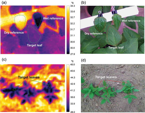
Stomatal conductance was measured on a fully expanded trifoliate leaf using a leaf porometer (SC-1, METER Environment, Pullman, USA). Then, thermal image of the same leaf was taken by a thermal camera (C2, FLIR systems, Wilsonville, USA) that scans wavebands at 7.5‒14 µm intervals with an image size of 80 × 60 pixels. The resolution of the temperature detection was 0.1°C. Emissivity was set at 0.99. The thermal image was taken together with dry and wet references that were cowpea leaves coated with vaseline and sprayed with water, respectively, according to Leinonen et al. (2006) (Figure 1(a) and (b)). Temperature at the central portion of the target leaf, dry reference, and wet reference were obtained from an original thermal image of 80 × 60 pixels using analysis software (FLIR Research IR MAX 4.40, FLIR systems, Wilsonville, USA). In all, a 128 data set (4 accessions, 8 time-points, and 4 replications) of stomatal conductance, leaf temperature, and reference temperatures was used to validate the thermal indicators of stomatal conductance. All measurements were performed only on the abaxial surface of the sampled leaves; nevertheless, we confirmed that the ratio of abaxial stomatal conductance to total conductance was not significantly different among the cowpea accessions under study (Table S1).

Figure 1. Infrared thermal image and RGB image of cowpea plants in the glasshouse experiment (a, b) and in the field experiment (c, d). In the glasshouse experiment, dry and wet references were taken together with the target leaf in a thermal image. In the field experiment, three plants were included in an image and the leaf temperature was detected for the top fully expanded leaves of each plant.

2.2. Field experiment

2.2.1. Plant materials and growth conditions

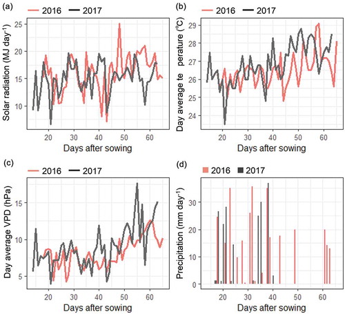
The same four accessions of cowpea used in the glasshouse experiment were grown in an experimental field at IITA during the cowpea growing season (September–November) in 2016 and 2017. The soil was a sandy loam with moderate acidity (pH 5.8–6.1). Sowing was done on 29 August 2016 and on 5 September 2017. Distance between plants was 20 cm and rows were spaced 75 cm apart for a planting density of 6.6 plants m⁻²; each experimental plot was 5.25 m × 6 m and consisted of seven rows with 31 plants per row, for a total of 217 plants per experimental plot. The field experiments were laid in a randomized block design with four replications. Weeding was conducted every week using a hand hoe, and no fertilizers were applied. Meteorological data for the experimental periods are summarized in Figure 1. Total precipitation, average minimum/maximum temperatures, and average solar radiation for the cowpea growing season were 414 mm, 22.3/30.3°C, and 14.9 MJ day⁻¹ in 2016, and 523 mm, 22.5/30.0°C, and 14.7 MJ day⁻¹ in 2017.

2.2.2. Measurements

Infrared thermal images of the cowpea plants were taken with the thermal camera between 10:00 and 12:00 h, every week from emergence to the beginning of maturity (i.e. 2‒8 weeks after sowing). Three contiguous plants were randomly selected within each experimental plot, and the corresponding thermal images were taken from a distance of 1 m above the plant for a resolution of 0.9 cm per pixel (Figure 1(c) and (d)). The temperature at the central point of a fully expanded trifoliate leaf was obtained for each of the three plants from a thermal image using the camera software. A total of 896 data sets of leaf temperature comprising 4 accessions, 3 plants, 4 replications, 7 time-points, and 2 years, were averaged for plants and replications, and merged into 56 sample data sets (4 accessions, 7 time-points, and 2 years). These data sets were used for calculating the indicators of stomatal conductance.

Simultaneously to the obtention of thermal images (once a week during 2‒8 weeks after sowing), leaf stomatal conductance was measured using the leaf porometer. These measurements were performed for a fully expanded trifoliate leaf on four plants per experimental plot, which were not the same as the plants used for thermal imaging. A total of 896 data sets of stomatal conductance consisting of 4 accessions, 4 plants, 4 replications, 7 time-points, and 2 years were averaged for plants and replications, and merged into 56 data sets (4 accessions, 7 time-points, and 2 years). These data sets were used to validate the thermal indices of stomatal conductance without having to use any reference temperatures.

Field meteorological conditions of air temperature, relative humidity, and precipitation were collected from the weather station at IITA. To measure short-wave solar radiation, the same device used in the glasshouse experiment was installed 2 m above the ground.

2.3. Indicator of stomatal conductance

2.3.1. Theoretical considerations

A new indicator of stomatal conductance (GsI) was developed through a modification of the theoretical equation. The latent heat flux (λE; W m⁻²) describing heat transfer related to transpiration from a leaf was described as

(1) $\lambda \mathrm{E}=\frac{{\mathrm{C}}_{\mathrm{p}}\rho }{\gamma }\left({\mathrm{e}}_{\mathrm{s}}-{\mathrm{e}}_a\right)\cdot {\mathrm{g}}_{\mathrm{v}}\cdot$(1)

where C_p is specific heat of the air (J kg⁻¹°C⁻¹), ρ is the air density (kg m⁻³), γ is the psychrometric constant (hPa°C⁻¹), and g_v (m s⁻¹) is the total conductance for water vapor transport from the leaf to the air. The g_v is the sum of stomatal conductance (g_s; m s⁻¹) and boundary layer conductance (g_a; m s⁻¹) for water vapor. In this equation, λE is proportional to the vapor pressure difference between the leaf surface (e_s; hPa) and the air (e_a; hPa). The term e_s–e_a is calculated from air temperature (T_a; °C), leaf surface temperature (T_s; °C), and relative humidity (RH; %). Saturated vapor pressure at temperature T (D_T; hPa) is calculated from Equation (2) based on Murray (1967). In a transpiring leaf, vapor pressure at the leaf surface was assumed to be at saturation level and was expressed as $e_s=D_{T_S}$. Hence, the air vapor pressure can be obtained from Equation (3).

(2) ${\mathrm{D}}_{\mathrm{T}}=6.108\mathrm{e}\mathrm{x}\mathrm{p}\left(\frac{17.3\mathrm{T}}{237.3+\mathrm{T}}\right)$(2)

(3) ${\mathrm{e}}_{\mathrm{a}}={\mathrm{D}}_{{\mathrm{T}}_{\mathrm{a}}}\cdot \frac{\mathrm{R}\mathrm{H}}{100}$(3)

Then, λE in Equation (1) is arranged using the energy balance model. The energy balance at the leaf surface is given by

(4) ${\mathrm{R}}_{\mathrm{n}}=\mathrm{H}+\lambda \mathrm{E}+\mathrm{G}+\mathrm{S}$(4)

where all units are W m⁻², and R_n is the net radiation and H is the sensible heat flux. G and S are heat flux to the ground and to the leaf, respectively, which are normally small and can be ignored. From Equations (1) and (4), g_v can be expressed as

(5) ${\mathrm{g}}_{\mathrm{v}}=\frac{\left({\mathrm{R}}_{\mathrm{n}}-\mathrm{H}\right)}{\left({\mathrm{e}}_{\mathrm{s}}-{\mathrm{e}}_{\mathrm{a}}\right)}\cdot \frac{\gamma }{{\mathrm{C}}_{\mathrm{p}}\rho }$(5)

To simplify this equation, the number of parameters was reduced by introducing the following assumptions; (i) Net radiation (R_n) is equal to the absorbed short-wave radiation (R_s), and H is much smaller than λE when transpiration occurs (Moncrieff et al., 1997; Page, Liénard, Pruett & Moffett, 2018). Therefore, the term R_n–H is proportional to R_s. (ii) Transpiration rate is mainly regulated by stomatal conductance (g_s) rather than boundary layer conductance (g_a) (Bunce, 1985; Meinzer & Grantz, 1991). Therefore, total conductance (g_v) is proportional to g_s. (iii) The psychrometric constant (γ) is generally used as a constant value. However, Loescher, Hanson and Ocheltree (2009) empirically estimated γ using chilled-mirror technologies and indicated that γ was much lower than the generally used value under humid conditions where the temperature difference between dry and wet bulbs is less than 12°C. Depending on this notion, we assumed that γ is proportional to vapor pressure deficit (VPD; hPa) calculated from Equation (6). In consideration of the above assumptions, the GsI is calculated according to Equation (7).

(6) $\mathrm{V}\mathrm{P}\mathrm{D}={\mathrm{D}}_{{\mathrm{T}}_{\mathrm{a}}}\left(1-\frac{\mathrm{R}\mathrm{H}}{100}\right)$(6)

(7) ${\mathrm{g}}_{\mathrm{s}}\propto \mathrm{G}\mathrm{s}\mathrm{I}=\frac{{\mathrm{R}}_{\mathrm{s}}}{\left({\mathrm{e}}_{\mathrm{s}}-{\mathrm{e}}_{\mathrm{a}}\right)}\cdot \frac{\mathrm{V}\mathrm{P}\mathrm{D}}{{\mathrm{C}}_{\mathrm{p}}\rho }$(7)

The units for GsI are °C m s⁻¹. The C_pρ is volumetric heat capacity of the air, and is used as a constant value of 1216 J m⁻³°C. For the calculation of GsI, T_s was determined from the thermal image, and T_a, RH, and R_s were obtained from meteorological data average values prevalent during the measurement period.

To compare the accuracy of GsI with other thermal indicators of stomatal conductance, temperature difference (T_a–T_s) and crop water stress index (CWSI) were also calculated. The CWSI uses both dry and wet reference temperatures indicated as T_dry and T_wet, respectively (Maes & Steppe, 2012).

(8) $\mathrm{C}\mathrm{W}\mathrm{S}\mathrm{I}=\frac{{\mathrm{T}}_{\mathrm{w}\mathrm{e}\mathrm{t}}-{\mathrm{T}}_{\mathrm{s}}}{{\mathrm{T}}_{\mathrm{w}\mathrm{e}\mathrm{t}}-{\mathrm{T}}_{\mathrm{d}\mathrm{r}\mathrm{y}}}$(8)

2.3.2. Comparison of g_s with the thermal indicators of stomatal conductance

To validate thermal indicators of stomatal conductance, values were compared to g_s measured by a porometer. Regression analysis was separately performed for each of the measuring time-points under different meteorological conditions in the glasshouse and the field experiments.

Coefficients of the regression line between g_s and GsI, T_a–T_s, or CWSI were estimated following the Bayesian model using measuring time-points as the hierarchical parameter. To compare the stability of the regressions among thermal indicators, all data of the indicators were standardized to a mean of 0 and a standard deviation of 1 before the analysis.

(9) $g_s\mathrm{\_}mean=a\left[\mathrm{k}\right]\times \mathrm{I}\mathrm{n}\mathrm{d}\mathrm{e}\mathrm{x}+b\left[\mathrm{k}\right]$(9)

(10) $x\left[\mathrm{k}\right]\mathrm{N}\mathrm{o}\mathrm{r}\mathrm{m}\mathrm{a}\mathrm{l}\left(x^{\prime },\sigma \mathrm{\_}x\right)$(10)

(11) ${\mathrm{g}}_{\mathrm{s}}\mathrm{N}\mathrm{o}\mathrm{r}\mathrm{m}\mathrm{a}\mathrm{l}\left(g_s\mathrm{\_}mean,\sigma \right)$(11)

where a[k] and b[k] were different for each sampling time-point. The number of k was 8 in the glasshouse experiment and 14 in the field experiment, corresponding to the total number of measuring time-points. The Index represents GsI, T_a–T_s, or CWSI. Here, we assumed that differences in the coefficients of the models among the measuring time-points followed a normal distribution. In Equation (10), x[k] represents each of a[k] and b[k] in Equation (9), and x′ and σ_x represent the mean and standard deviation of the normal distribution of x[k]. Additionally, g_s was considered to follow a normal distribution with an average of g_s_mean and a standard deviation of σ (Equation (11)). The posterior distributions of all coefficients were generated by the Markov chain Monte Carlo (MCMC) method. The MCMC algorithm was set at 3000 steps for iteration and 500 steps for warm-up; there were four chains and the total sample size was 10,000. The convergence was confirmed by visualization of a trace plot and ‘R hat’ (potential scale reduction factor on split chains). The Bayesian analysis was performed using the statistical software R version 3.4.1 with the package ‘rstan’.

2.4. Evaluation of genotypic variation of stomatal conductance using GsI

GsI was evaluated for 248 accessions of the cowpea mini-core subset from the world cowpea germplasm collection developed at IITA (Fatokun et al., 2018). Field sowing was done on 3 September 2018. Each accession occupied a 2 m line plot with 20 cm between plants and rows 1.5 m apart. The plots were arranged in a randomized block design with three replications. Weeding was conducted using a hand hoe and again, no fertilizers were applied. Total precipitation, average minimum/maximum temperatures, and average solar radiation for the growing period were 154 mm, 22.6/30.8°C, and 15.2 MJ day⁻¹. Thermal images were taken at 5 and 8 weeks after sowing, corresponding to the vegetative growth stage and beginning of maturity, respectively. Measurement of leaf temperature and calculation of GsI were performed as described above. GsI were calculated for each of the three replications and averaged.

3. Results

3.1. Validation of the thermal indicators in the glasshouse experiment

Stomatal conductance varied from 0.05 to 0.56 mol m⁻² s⁻¹ over the 8 measuring time-points. The highest values were observed in the afternoon at 51 DAS, when R_s and T_a were higher during the measuring time-points (Table 1). However, the lowest values were observed in the morning at 14 DAS, when VPD and T_a were relatively lower than at any other sampling time-points.

The values of g_s were compared with thermal indicators of stomatal conductance with and without reference temperature (Figure 2(a, c, and e)). For all thermal indicators, variation within any measurement date correlated well with g_s. However, when the values of T_a–T_s and CWSI were compared among different measurement dates, the afternoon (PM) values of g_s were overestimated, relative to morning (AM) values. Among measurement dates, large differences were observed in subsequent distributions of the slope (a) and constant (b) estimated from the Bayesian analysis. As for the relationship between T_a–T_s and g_s, higher values for the slope (a) were observed at 49 and 51 DAS, and higher values for constant (b) were observed at 47 DAS. On the other hand, in the case of the relationship between CWSI and g_s, the values for the slope (a) were relatively stable, but the values for constant (b) varied among sampling time-points. The higher values were observed in the afternoon, when VPD and T_a were higher than that in the morning. Compared with T_a–T_s and CWSI, GsI showed stable values for both slope (a) and constant (b) throughout the different sampling time-points (Figure 2(b)).

Figure 2. Summary of the regression analysis between stomatal conductance and the thermal indicators in the glasshouse experiment. The relationship (a, c, e) and posterior distributions of the coefficients (b, d, f) are separately shown for each measuring time-point under different meteorological conditions. The regressions between stomatal conductance and GsI (a, b): between stomatal conductance and air-leaf temperature difference (T_a−T_s) (c, d): between stomatal conductance and crop water stress index (CWSI) (e, f). Bar with each point in the scatter plot indicates the 95% interval of the predicted distribution. The box-plots of the coefficients for slope (a) and for constant (b) were generated from 10,000 Markov chain Monte Carlo (MCMC) samples for each measuring time-point.

3.2. Field experiment

3.2.1. Meteorological conditions

Meteorological conditions were largely different between the two years of study (Figure 3). There were intermittent cloudy days with no precipitation in 2017 that led to the low total precipitation and solar radiation, especially at the late vegetative growth, 5‒8 weeks after sowing. VPD was higher in 2017 than in 2016 throughout the growth period. Daily average wind speed during the experimental period was lower than 1.0 m s⁻¹ in both years.

Figure 3. Meteorological conditions during the field experiment in 2016 and 2017. Weekly average values from 2–8 weeks after sowing are shown for (a) solar radiation, (b) daytime temperature (6:00‒18:00), and (c) daytime vapor pressure deficit (6:00‒18:00). Weekly cumulative values are shown for (d) precipitation.

3.2.2. Validation of the thermal indicators in the field experiment

The g_s values were largely different depending on the date of measurement, and varied from 0.19 to 0.93 mol m⁻² s⁻¹ (Figure 4). The highest values were observed at 58 DAS in 2016, when R_s and T_a were highest during the two seasons. On the other hand, the lowest value was observed at 14 DAS in 2017, when R_s and T_a were relatively lower than at any other measuring time-point. In 2017, the values of g_s tended to be smaller than those in 2016, with all values being under 0.5 mol m⁻² s⁻¹.

Figure 4. Summary of the regression analysis between stomatal conductance and the thermal indicators in the field experiment. The relationships (a, c) and posterior distributions of the coefficients (b, d) are separately shown for each measuring time-point under different meteorological conditions. Regressions: between stomatal conductance and GsI (a, b): between stomatal conductance and air-leaf temperature difference (T_a−T_s) (c, d). Bars with each point in the scatter plot are the 95% interval of the predicted distribution. The box-plots of the coefficients were generated from 10,000 Markov chain Monte Carlo (MCMC) samples for each time-point.

The values of g_s were compared with the indicators without reference temperatures because of the difficulty for the field application of thermal indicators with reference temperatures. Figure 4(c) shows that g_s values were largely different even when T_a–T_s were the same; in 2016, g_s was generally overestimated in comparison with 2017. Further, in both years, T_a–T_s varied largely even when g_s values were the same. Posterior distributions of the coefficients for the regression line between T_a–T_s and g_s are shown in Figure 4(d). The values for constants (b) varied largely among measurement dates, whereas the values for the slopes (a) were stable. The greater constants were observed at 29, 51, and 58 DAS in 2016, in correspondence with the dates with higher solar radiation. However, the lower values were observed at 24 DAS in 2016 and at 14 and 35 DAS in 2017, corresponding to the dates with lower VPD. In contrast to T_a–T_s, over or underestimation of g_s among measurement dates were much smaller in GsI (Figure 4(a)), and the coefficients for the slope and constant of the regression line were more stable (Figure 4(b)). All the coefficients above converged and showed that the R hat was <1.1.

3.3. Genotypic variation of stomatal conductance for cowpea germplasm

The distribution of GsI values for the 248 cowpea accessions were separately shown for three groups genetically classified by Fatokun et al. (2018) (Figure 5). The values of GsI at 5 weeks after sowing varied from 0.1 to 0.3 with a mode of 0.2, corresponding to approximate stomatal conductance values in the range of 0.2 to 0.6 mol m⁻² s⁻¹ (Figure 5(a)). The accessions with GsI >0.2 were mostly in groups 2 and 3, whereas accessions in group 1 were characterized by GsI <0.2. At 8 weeks after sowing, distributions of GsI became flat and showed no specific peaks (Figure 5(b)). GsI of all groups decreased with the beginning of plant senescence. At this point, the number of accessions showing GsI <0.15 increased, although some still maintained GsI >0.2.

4. Discussion

A novel proxy of stomatal conductance, GsI, was calculated using a simplified equation with four variables, namely, leaf and air temperature, relative humidity, and solar radiation. Except for leaf temperature, all other variables can be obtained from continuous-measurement devices installed near the field; thus, an evaluator only needs to take a thermal image for each measurement. As GsI calculation does not require any reference temperature, the time for photographing is much shorter than that for evaluations with reference temperatures. Therefore, this new method is suitable for rapidly evaluating a large plant population, such as a set of genetic resources and cross-populations for genetic analysis.

In comparison with other indicators, the advantage of GsI is its stable relationship with g_s. The values of GsI rendered almost the same slopes and constants in the regressions to g_s even under different meteorological conditions in both glasshouse and field experiments (Figures 2 and 4). The T_a–T_s and CWSI showed a good relationship with g_s under similar meteorological conditions, but the slope or constant of the regression were largely different when the meteorological conditions were largely different, a finding that agreed with results reported by a previous study (Agam, Cohen, Alchanatis & Ben-Gal, 2013). Its stable relationship with g_s makes it possible to compare GsI values among different environments. Another advantage of GsI is the flexibility for modification. Because the calculation of GsI is based on the theoretical equation of g_s, other parameters, such as sensible heat flux or boundary layer conductance, can be easily added if so desired. When the evaluation was performed under similar conditions of solar radiation, air temperature, or air humidity, constant values can be applied for these parameters instead of the measured values.

As we targeted single leaves on each sample plant, whose thermal image was taken from a distance of only one meter above, an image of 4800 pixels was believed to be enough for leaf temperature determination. Therefore, although several types of high-resolution thermal cameras are commercially available, we used a low-cost thermal camera of a relatively low resolution (60 × 80 pixels). Additionally, the use of such low-cost camera allows the method to be used for trait evaluations, not only as part of basic scientific studies, but also for local agronomic and breeding programs, especially in developing countries. Further, multiple low-cost thermal cameras can be used simultaneously to reduce the evaluation time, although, in this case, temperature calibration is needed to adjust the reading temperature among the different cameras.

Compared to the glasshouse experiment, GsI values calculated in the field experiment were biased towards lower values. This is because the air temperature and relative humidity data used for the calculation were different in the two experiments. Air temperature and humidity recorded at the field weather station were not identical with that immediately around the leaf surface in the field. However, as long as such differences do not vary to any large extent, they will not affect the calculation of GsI, and comparison of the values among environments is possible. This was clearly confirmed by the results of our field experiment, which showed that GsI values correlated highly with measured g_s throughout the two years of study. When the evaluator needs to compare GsI values calculated from meteorological data provided by different devices, calibration is needed to adjust the difference in meteorological data among the measuring instruments used in each case, although this is a common feature for any thermal indicator of stomatal conductance.

Under field conditions, wind sometimes disturbs accurate estimation of stomatal conductance based on leaf temperature because the boundary layer resistance to heat transfer is highly affected by wind speed. Leinonen et al. (2006) reported that the error ratio of the calculated g_s under conditions of low wind speed becomes higher than the corresponding ratio under conditions of high wind speed. However, the same authors also reported that the wind effect is prominent only for the lower range of g_s values, and that such effect becomes much smaller for g_s larger than 0.2 mol m⁻² s⁻¹. As measured g_s values ranged from 0.19 to 0.93 mol m⁻² s⁻¹ in the field experiment (Figure 4), the differences in wind speed might have had a slight effect on the calculations of GsI; hence, GsI is not suitable for estimating low g_s values, although this issue was not thoroughly examined in this study. The GsI is most accurate as a g_s estimate in the range from moderate to high g_s values (approximately, >0.2 mol m⁻² s⁻¹), in which GsI is a useful indicator to estimate plant growth and water status.

The stable relationship between GsI and g_s shown in Figures 2 and 4, indicated that the relationship was also stable for the different cowpea genotypes tested in this study. This is because measurements were conducted only on horizontal leaves (Figure 1), and differences in leaf morphology and orientation, which affect leaf temperature (Leigh, Sevanto, Close & Nicotra, 2017; Media, Sobrado & Herrera, 1978), were not distinguished among accessions. We found large genetic variability for GsI estimates among the 248 accessions of cowpea genetic resources under study. Cowpea is grown in diverse environments ranging from humid to arid regions (Ehlers & Hall, 1997), and thus stomatal responses to a given environment are thought to differ depending on the origin of the genotype. Values of GsI at 8 weeks after sowing tended to be lower than those obtained at 5 weeks after sowing due to the start of plant senescence (Figure 5). Thus, GsI evaluation at vegetative growth stage is suitable to know the maximum values of stomatal conductance for each accession. The accessions with higher GsI values at 5 weeks after sowing were mostly recorded in accessions belonging in groups 2 and 3 (Figure 5(a)). More than 90% of the accessions in group 2 are native to West and Central Africa (Fatokun et al., 2018). Among accessions in group 2, significantly higher GsI values were calculated for TVu13388, TVu4783, and TVu14539, which originated in Burkina Faso, Niger, and Mali, respectively. These accessions were thought to have a higher degree of genetic control on g_s. Such genotypic differences might be associated with the corresponding differences in the ability for environmental adaptation, which ultimately relate to yield variability (Lizana et al., 2006).

Because reference temperatures are not needed for calculating GsI, this indicator is easy to apply for field measurement in many plants and at frequent measuring time-points, although the GsI is most accurate as a g_s estimate in the range from moderate to high g_s values. Determination of g_s using GsI provides important physiological information related to plant responses to the environment, and will help to identify superior genotypes with high adaptability to specific target environments. Combined with genomic information, such as full genome sequence, which is available for cowpea (Muñoz-Amatriaín, Mirebrahim & Xu et al., 2017), rapid evaluation of g_s will serve to accelerate cowpea breeding programs, as shown in other major crops (Liu et al., 2011).

Acknowledgments

We thank Dr Ryo Matsumoto at IITA Yam breeding unit for assistance in field management, and Ms. Obaude Oyebola O. and Mr. Oyedele Sunday O. for their assistance in the field evaluation.

Disclosure statement

No potential conflict of interest was reported by the authors.

Supplementary material

Supplemental data for this article can be accessed here.

Additional information

Funding

This work was funded from the JIRCAS research program ‘Development of sustainable technologies to increase agricultural productivity and improve food security in Africa’.

References

- Agam, N., Cohen, Y., Alchanatis, V., & Ben-Gal, A. (2013). How sensitive is the CSWI to changes in solar radiation? International Journal of Remote Sensing, 34, 6109–6120.
- Brenner, A. J., & Jarvis, P. G. (1995). A heated leaf replica technique for determination of leaf boundary layer conductance in the field. Agricultural and Forest Meteorology, 72, 261–275.
- Bunce, J. A. (1985). Effect of boundary layer conductance on the response of stomata to humidity. Plant, Cell and Environment, 8, 55–57.
- Costa, J. M., Grant, O. M., & Chaves, M. M. (2013). Thermography to explore plant–environment interactions. Journal of Experimental Botany, 64, 3937–3949.
- Egea, G., Padilla-Diaz, C. M., Martinez-Guanter, J., Fernandez, J. E., & Perez-Ruiz, M. (2017). Assessing a crop water stress index derived from aerial thermal imaging and infrared thermometry in super high-density olive orchards. Agricultural Water Management, 187, 210–221.
- Ehlers, J. D., & Hall, A. E. (1997). Cowpea (Vigna unguiculata L. Walp.). Field Crops Research, 53, 187–204.
- Fatokun, C., Girma, G., Abberton, M., Gedil, M., Unachukwu, N., Oyatomi, O., … Boukar, O. (2018). Genetic diversity and population structure of a mini-core subset from the world cowpea (Vigna unguiculata (L.) Walp.) germplasm collection. Scientific Reports, 8, 16035.
- Fischer, R. A., Rees, D., Sayre, K. D., Lu, Z. M., Condon, A. G., & Saavedra, A. L. (1997). Wheat yield progress associated with higher stomatal conductance and photosynthetic rate, and cooler canopies. Crop Science, 38, 1467–1475.
- Flexas, J., & Medrano, H. (2002). Drought-inhibition of photosynthesis in C3 plants: Stomatal and non-stomatal limitations revisited. Annals of Botany, 89, 183–189.
- Guo, J. X., Tian, G. L., Zhou, Y., Wang, M., Ling, N., Shen, Q. R., & Guo, S. W. (2016). Evaluation of the grain yield and nitrogen nutrient status of wheat (Triticum aestivum L.) using thermal imaging. Field Crops Research, 196, 463–472.
- Han, M., Zhang, H. H., DeJonge, K. C., Comas, L. H., & Trout, T. J. (2016). Estimating maize water stress by standard deviation of canopy temperature in thermal imagery. Agricultural Water Management, 177, 400–409.
- Jones, H. G. (1999). Use of thermography for quantitative studies of spatial and temporal variation of stomatal conductance over leaf surfaces. Plant, Cell and Environment, 22, 1043–1055.
- Jones, H. G. (2004). Application of thermal imaging and infrared sensing in plant physiology and ecophysiology. Advances in Botanical Research, 41, 108–155.
- Leigh, A., Sevanto, S., Close, J. D., & Nicotra, A. B. (2017). The influence of leaf size and shape on leaf thermal dynamics: Does theory hold up under natural conditions? Plant, Cell and Environment, 40, 237–248.
- Leinonen, I., Grant, O. M., Tagliavia, C. P. P., Chaves, M. M., & Jones, H. G. (2006). Estimating stomatal conductance with thermal imagery. Plant, Cell and Environment, 29, 1508–1518.
- Lima, R. S. N., Garcia-Tejero, I., Lopes, T. S., Costa, J. M., Vaz, M., Duran-Zuazo, V. H., & Campostrini, E. (2016). Linking thermal imaging to physiological indicators in Carica papaya L. under different water regimes. Agricultural Water Management, 164, 148–157.
- Liu, Y., Subhash, C., Yan, J., Song, C., Zhao, J., & Li, J. (2011). Maize leaf temperature responses to drought: Thermal imaging and quantitative trait loci (QTL) mapping. Environmental and Experimental Botany, 71, 15–165.
- Lizana, C., Wentworth, M., Martinez, J. P., Villegas, D., Meneses, R., Murchie, E. H., & Pinto, M. (2006). Differential adaptation of two varieties of common bean to abiotic stress: I. Effects of drought on yield and photosynthesis. Journal of Experimental Botany, 57, 685–697.
- Loescher, H. W., Hanson, C. V., & Ocheltree, T. W. (2009). The psychrometric constant is not constant: A novel approach to enhance the accuracy and precision of latent energy fluxes through automated water vapor calibrations. Journal of Hydrometeorology, 10, 1271–1284.
- Lu, Z., Percy, R. G., Qualset, C. O., & Zeiger, E. (1998). Stomatal conductance predicts yield in irrigated Pima cotton and bread wheat grown at high temperatures. Journal of Experimental Botany, 49, 453–460.
- Maes, W. H., & Steppe, K. (2012). Estimating evapotranspiration and drought stress with ground-based thermal remote sensing in agriculture: A review. Journal of Experimental Botany, 63, 695–709.
- Media, E., Sobrado, M., & Herrera, R. (1978). Significance of leaf orientation for leaf temperature in an Amazonian sclerophyll vegetation. Radiation and Environmental Biophysics, 15, 131–140.
- Medrano, H., Escalona, J. M., Bota, J., Gulías, J. & Flexas, J. (2002). Regulation of photosynthesis of C3 plants in response to progressive drought: Stomatal conductance as a reference parameter. Annals of Botany, 89, 895–905.
- Meinzer, F. C., & Grantz, D. A. (1991). Coordination of stomatal, hydraulic, and canopy boundary layer properties: Do stomata balance conductance by measuring transpiration? Physiologia Plantarum, 83, 324–329.
- Moncrieff, J. B., Massheder, J. M., Bruin, H., Elbers, J., Friborg, T., Heusinkveld, B., & Verhoef, A. (1997). A system to measure surface fluxes of momentum, sensible heat, water vapour and carbon dioxide. Journal of Hydrology, 188–189, 589–611.
- Muñoz-Amatriaín, M., Mirebrahim, H., Xu, P., Wanamaker, S. I., Luo, M., Alhakami, H., ... Close, T. J. (2017). Genome resources for climate-resilient cowpea, an essential crop for food security. The Plant Journal, 89, 1042–1054.
- Murray, F. W. (1967). On the computation of saturation vapor pressure. Journal of Applied Meteorology, 6, 203–204.
- Oren, R., Sperry, J. S., Katul, G. G., Pataki, D. E., Ewers, B. E., Phillips, N., & Schäfer, K. V. R. (1999). Survey and synthesis of intra- and interspecific variation in stomatal sensitivity to vapour pressure deficit. Plant, Cell and Environment, 22, 1515–1526.
- Padhi, J., Misra, R. K., & Payero, J. O. (2012). Estimation of soil water deficit in an irrigated cotton field with infrared thermography. Field Crops Research, 126, 45–55.
- Page, G. M. F., Liénard, J. F., Pruett, M. J., & Moffett, K. B. (2018). Spatiotemporal dynamics of leaf transpiration quantified with time-series thermal imaging. Agricultural and Forest Meteorology, 256–257, 304–314.
- Stoll, M., Schultz, H. R., & Berkelmann-Loehnertz, B. (2008). Exploring the sensitivity of thermal imaging for Plasmopara viticola pathogen detection in grapevines under different water status. Functional Plant Biology, 35, 281–288.
- Takai, T., Yano, M., & Yamamoto, T. (2010). Canopy temperature on clear and cloudy days can be used to estimate varietal differences in stomatal conductance in rice. Field Crops Research, 115, 165–170.
- Yu, Q., Zhang, Y., Liu, Y., & Shi, P. (2004). Simulation of the stomatal conductance of winter wheat in response to light, temperature and CO2 changes. Annals of Botany, 93, 435–441.