Predicting rice (Oryza sativa L.) canopy temperature difference and estimating its environmental response in two rice cultivars, ‘Koshihikari’ and ‘Takanari’, based on a neural network

ABSTRACT

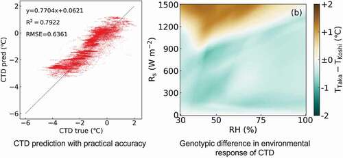
Canopy photosynthesis is an important component of biomass production in field-grown rice (Oryza sativa L.). Although canopy temperature differences (CTD) provide important information for evaluating canopy photosynthesis, the measurement of CTD is still a labor-intensive task. Therefore, we designed this study to establish a model for predicting CTD under different field conditions using meteorological data and evaluated the environmental response of CTD using the established model. Our study collected 2,056,264 CTD data points from two rice cultivars having different photosynthetic capacities, ‘Koshihikari’ and ‘Takanari’, and then used these data to create a novel model using a neural network (NN). The input variables were limited to meteorological data, and the output variable was set to CTD. The established NN model produced a prediction accuracy of R² = 0.792 and RMSE = 0.605°C. We then used this NN model to simulate the CTD response of the Koshihikari and Takanari cultivars in response to various environmental changes. These predictions revealed that Takanari had a lower CTD than Koshihikari when exposed to high relative humidity (RH) or low to moderate solar radiation (R_s). In contrast, the CTD of Koshihikari tended to be lower than that of Takanari under lower RH or higher R_s. This result implies that the advantages of the single-leaf gas exchange system in Takanari can be mitigated under extremely high-VPD conditions. Thus, our new method may provide a powerful tool to gain a better understanding of gas exchange, growth processes, and varietal differences in rice cultivated under field conditions.

Graphical Abstract

KEYWORDS:

• Rice (oryza sativa L.)
• koshihikari
• takanari
• canopy temperature difference
• neural network
• environmental response

Introduction

Photosynthesis is a critical factor in plant biomass production. Numerous studies have investigated the relationship between photosynthetic activity, biomass production, and final crop yield (Long et al., 2006; Wu et al., 2019; Yoon et al., 2020; Zhu et al., 2010). In field settings, crops grow as canopies under changing meteorological conditions, thus it is not surprising that various methods for evaluating canopy photosynthesis have been developed over time. These include the canopy photosynthesis model (Anten, 1997; Johnson & Thornley, 1984; Li et al., 2021; Monsi & Saeki, 2005), eddy covariance (Alberto et al., 2014; Ohtaki, 1984), and assimilation chambers (Burkart et al., 2007; Drake & Leadley, 1991; Katsura et al., 2006; Song et al., 2016). In addition, photosynthetic activity in constantly changing environments has been intensively assessed in rice (Adachi et al., 2019a; Qu et al., 2016; Taniyoshi et al., 2020; Yamori et al., 2020), soybean (Soleh et al., 2016; Tanaka et al., 2019), and other field crops (Salter et al., 2019; De Souza et al., 2020; Taylor & Long, 2017). However, the long-term monitoring of canopy photosynthesis under field conditions remains challenging.

Photosynthesis can be evaluated using thermal imaging techniques as leaf/canopy transpiration is reflected in leaf/canopy surface temperature (Gates, 1968; Jones, 2014). Given this, many studies have evaluated changes in the canopy surface temperature to evaluate the crop canopy status of open fields. Takai et al. (2010) revealed that canopy surface temperature is strongly related to the photosynthetic rate and stomatal conductance of the outer leaves, while Horie et al. (2006) reported that canopy diffusive conductance under field conditions could be estimated based on the surface temperature of both shaded and sunlit canopies. The canopy transpiration rate was estimated in short-time intervals based on the canopy surface temperature and the heat balance model (Monteith & Unsworth, 2013) for rice (Kondo et al., 2021), soybean (Hou et al., 2019), and cotton (Jones et al., 2018). All these techniques assume that the leaf surface temperature is strongly affected by the latent heat flux of transpiration. Therefore, canopy temperature difference (CTD), represented by the difference between air and canopy surface temperature, is fundamental to the use of thermal imaging techniques. However, the measurement of CTD remains a challenging task because of the labor-intensive and technically sophisticated evaluations required to complete these evaluations. Furthermore, the use of thermal imaging techniques has spatiotemporal limitations. The canopy surface temperature measured using thermal imaging devices are typically evaluated as a single image, and the capturing range of thermal imaging devices is limited. Even though this spatial limitation can partly be overcome by combining with unmanned aerial vehicle, it is difficult to take continuously in short-time intervals. To apply thermal imaging techniques for evaluations of plants cultivated in a field with greater practicality, these limitations need to be overcome.

Micrometeorological conditions strongly affect canopy gas exchange (Jones, 2014). For instance, favorable temperatures and strong radiation generally accelerate photosynthesis (Choudhury, 1987; Yamori et al., 2014), which leads to stomatal opening and greater transpiration. Furthermore, air humidity affects stomatal aperture and transpiration rates (Monteith, 1995; Morison & Gifford, 1983). Thus, the activity of canopy gas exchange affects the canopy surface temperature and CTD, and it can be assumed that CTD can be estimated from micrometeorological data. Meteorological data are universally utilized in the field of agriculture, easy to access, can be collected in short-time intervals, and cover wide area of lands. Given this, the evaluation of meteorological data may be advantageous to realize easier estimation of CTD and transpiration, thus reducing costs and overcoming the spatiotemporal limitations in the use of thermal imaging techniques.

Neural networks (NNs) are intensively being applied in the field of crop science. For example, NNs have been used to help detect crop diseases (Mujahidin et al., 2021), predict biomass production (Jin et al., 2020; Ma et al., 2019), and grain yield (Das et al., 2018; Haghverdi et al., 2018; Nevavuori et al., 2019; Tanaka et al., 2021). In fact, some reports have even described using NN to estimate crop transpiration rates (Nam et al., 2019; J. Fan et al., 2021). However, these studies were conducted at a limited scale and had difficulties translating these results to large-scale field conditions. The use of thermal imaging techniques may solve these problems to some extent. In addition, to the best of our knowledge, ours is the first study designed to evaluate the application of NN to predict CTD in rice (Oryza sativa L.). The major reason for this is that the accumulation of data describing changes in the canopy surface temperature is a labor-intensive task. We collected the canopy surface temperatures of rice and the corresponding micrometeorological data at 2,056,264 points by establishing a system for estimating rice canopy transpiration rate over short time intervals (Kondo et al., 2021). We then used these data to develop an NN-mediated model to estimate CTD in an effort to increase accuracy and simplify these kinds of evaluations. Besides, the CTD prediction model based on big data may cancel noises/errors caused by fluctuations of weather conditions (e.g. wind velocity, air temperature). This advantage may contribute to extracting physiological responses to the variations of weather conditions more clearly in rice.

The gas exchange of and genotypic differences in rice under either steady state or simple environmental conditions have been reported numerous times (Ikawa et al., 2017; Qu et al., 2016; Yamori et al., 2020). Many previous studies have reported that the saturated photosynthetic rate of a single indica leaf from the ‘Takanari’ cultivar was significantly higher than that of various japonica cultivars, including ‘Koshihikari’ (Adachi et al., 2019b; Hirasawa et al., 2010; Takai et al., 2010; Taylaran et al., 2011). However, little information has been published regarding its canopy level gas exchange and genotypic differences in response to various meteorological conditions. This study focused on two rice cultivars, Koshihikari, the most popular cultivar in Japan, and Takanari, a cultivar having high photosynthetic capacities. With the model established to predict CTD from micrometeorological data, the environmental responses of CTD in these two cultivars under virtual meteorological conditions can be evaluated or simulated. Thus, our model may be useful in revealing differences in the environmental response of the canopy gas exchange in both Koshihikari and Takanari.

The aim of this study was to establish a less laborious method to predict CTD and then to evaluate the difference of environmental responses in two rice cultivars, Koshihikari and Takanari. We first developed an NN model to predict CTD using micrometeorological data for two rice cultivars, Koshihikari and Takanari, and the accuracy of the model was evaluated by comparison with two popular regression methods: multiple linear regression (MLR) and partial least squares regression (PLSR). Different CTD values produced under different meteorological conditions were then simulated for both cultivars and the results of these simulations were then used to evaluate genotypic differences in the response of these cultivars to changing environmental conditions. These experiments allowed us to produce a novel methodology for the easy estimation of CTD and evaluation of genotypic differences in environmental responses using micrometeorological data.

Materials and methods

Plant materials

Koshihikari and Takanari were cultivated in a paddy field at the Graduate School of Agriculture, Kyoto University, Kyoto, Japan (35° 2ʹ N, 135° 47ʹ E, 65 m altitude) in 2017, 2018, and 2019 with seeds being sown on April 20, 23 April 2017, 2018, and 19 April 2019, and the seedlings transplanted on May 16, 18 May 2017, 2018, and 17 May 2019. The planting density was 22.2 plants·m⁻² and we used 60 kg N ha⁻¹, 47 kg P ha⁻¹, and 56 kg K·ha⁻¹ as the basal dressing across all 3 years. In 2018 and 2019, 40 kg N·ha⁻¹, 31 kg P·ha⁻¹, and 37 kg K·ha⁻¹ were additionally applied as top dressings at the beginning of July. Weeds, diseases, and insects were strictly controlled, and the field was fully irrigated throughout the growing season.

Data collection

Micrometeorological data from the paddy field were measured using a meteorological data acquisition system from July 18th to 25th over 3 years at 1-s intervals, except for 24 July 2019, because of serious problems with the device. The air temperature (T_a) and relative humidity (RH) were recorded in 2017, using a temperature and relative humidity probe (CS215, Campbell Scientific, Inc., USA) with an aspirated radiation shield. Solar radiation (R_s) was recorded using an albedo meter (PCR-3, Kipp & Zonen, Netherlands). These instruments were set approximately 2 m above the ground (1 m above the canopy) and connected to a data logger (CR-1000; Campbell Scientific, Inc.). In 2018 and 2019, T_a and RH were recorded using a composite meteorological sensor (WS500; EKO Instruments, Japan) while R_s was recorded using a pyranometer (MS802; EKO Instruments, Japan). All sensors were set at the same height as in 2017 and were connected to a data logger (GL840, GRAPHTEC Co., Japan).

In all 3 years, the canopy surface temperature (T_c) was recorded using an infrared thermal imaging camera (InfReC S30, Nippon Avionics Co., Ltd., Japan) with a resolution of 160 × 120 pixels, with a spectral range of 8–13 μm, and thermal sensitivity of less than 0.2°C at 30°C. The camera was placed 16 m from the paddy field and 7 m above the ground with an elevation of 24°. Thermal images were then recorded every second and all plots were placed in a single image. T_c was corrected using reference temperatures and a temperature reference board was placed adjacent to the experimental field. The white felt was attached to a 60 × 40 cm wooden board and the surface temperature of the reference board was simultaneously recorded using a thermometer (TR-52i, T&D Corporation, Japan) and thermal imaging camera. The difference in these two data points was then used to correct the temperature drift of the thermal imaging camera. Our modeling assumed that this corrected for changes in canopy surface emissivity. Once corrected, we extracted the mean T_c value from each thermal image with four, two, and three replications in 2017, 2018, and 2019, respectively. CTD was then calculated using the following equation:

(1) $CTD=T_c-T_a$(1)

Data preprocessing, model establishment, and prediction

The distribution of all observed CTD data is shown in Figure 1(a) with each datasets classified as one of three categories: training, validation, and prediction, as shown in Figure 1(b). All parameters were normalized as follows:

Figure 1. (a) Histogram showing the distribution of all the observed CTD data points, (b) tabular representation of the dataset classification into Training, Validation, and Prediction subsets.

(2) $V_{norm}=\frac{V+\alpha }{V_{max}-V_{min}}$(2)

where V_norm is the value after normalization, V is the observed value, α is the correction term, V_max is the maximum observed value, and V_min is the minimum observed value. The parameters for normalizing each variable on a 0–1 scale are shown in Table 1. After this preprocessing, the model was established using three computational methods: MLR, PLSR, and NN, using the training and validation datasets. The input variables were T_a, RH, and R_s, and the output variable was CTD. The MLR and PLSR models were established using the scikit-learn library in Python, version 3.8.5, while the NN model was established using the Neural Network Console software (version 2.0 (Sony Network Communications Inc., Japan). First, the model structure was automatically determined using a structure search function in the Neural Network Console software using the Koshihikari dataset. The model structure with the least validation error was then selected (Figure 2). We then used this structure to train the model for both the Koshihikari and Takanari datasets. In both the structure search and training, the loss function was expressed as a squared error, and the optimizer was Adam. The batch size and learning rate were set as 512 and 0.0001, respectively. The learning process was used to minimize the errors between the estimated and observed CTDs in the training and validation datasets. The epoch size was set to 50, and the validation error was calculated every two epochs. This training revealed that the lowest validation error was observed in the 12th epoch in Koshihikari and the 20th epoch in the Takanari datasets. The model with the least validation error was then saved for each cultivar and used in all the downstream analyses. We then confirmed the efficacy of these models by using them to predict the CTD values for each strain on 22 July 2017, and 21 July 2018, respectively.

Figure 2. The structure of the model for predicting canopy transpiration rates. Each component can be explained as: ELU | Exponential Linear Unit, PReLU | Parametric Reflected Linear Unit, SELU | Scaled Exponential Linear Unit, and Squared Error | Output Layer minimizing the squared error. The numbers next to the Fully Connected Layers represent the number of dimensions.

Table 1. Representation of the minimum and maximum values (V_min,V_max, respectively) and correction term (α) for each as applied in the normalization.

Variable	Unit	Vmin	Vmax	α
Ta	°C	20	40	−20
RH	%	0	100	0
Rs	W m^−2	0	1500	0
CTD	°C	−10	10	10

Analysis

Prior to completing these predictions, we exposed our data to a correlation analysis focusing on the relationships between T_a, RH, R_s, CTD in Koshihikari, and CTD in Takanari. We then used the predictions from the MLR, PLSR, and NN models to determine the coefficient of determination (R²) and root mean squared error (RMSE) for the observed versus predicted CTD values. We then evaluated CTD prediction under virtual meteorological conditions using our NN model. These simulations were completed using RH and R_s values ranging from 30% to 100% and 0 to 1500 W m⁻², respectively. The T_a was fixed at one of three positions: 25°C, 30°C, or 35°C, and then used to predict CTD for both Koshihikari and Takanari using these parameters. Once completed, the simulated CTD values were compared and the difference in CTD between Koshihikari and Takanari (T_Taka – T_Koshi) was defined by the equation below:

(3) $T_{Taka}-T_{Koshi}=CT{D}_{Taka}-CT{D}_{Koshi}$(3)

where CTD_Taka and CTD_Koshi represent the CTDs of Takanari and Koshihikari, respectively. All analyses were conducted in Python (Van Rossum & Drake, 2009).

Results

Meteorological conditions

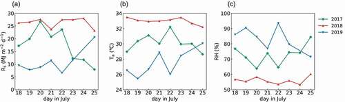
The mean daytime T_a, mean RH, and cumulative R_s from 18 to 25 July in 2017, 2018, and 2019 are shown in Figure 3. The mean T_a ranged from 25.43°C on 19 July 2019, to 33.48°C on 18 July 2018. The mean RH ranged from 53.21% on 24 July 2018, to 93.55% on 22 July 2019. The cumulative R_s ranged from 6.56 MJ·m⁻²·d⁻¹ on 22 July 2019, to 28.00 MJ·m⁻²·d⁻¹ on 24 July 2018. Generally, 2018 was characterized as hot and dry, while 2019 was cool and humid. 2017 displayed a larger variance in weather and ran the full gambit of these conditions.

Figure 3. (a) Daily cumulative solar radiation (R_s), (b) mean air temperature (T_a), and (c) mean relative humidity (RH) for the daytime between July 18 and July 25 in 2017, 2018, and 2019, except 24 July 2019. The green, red, and blue lines represent 2017, 2018, and 2019, respectively.

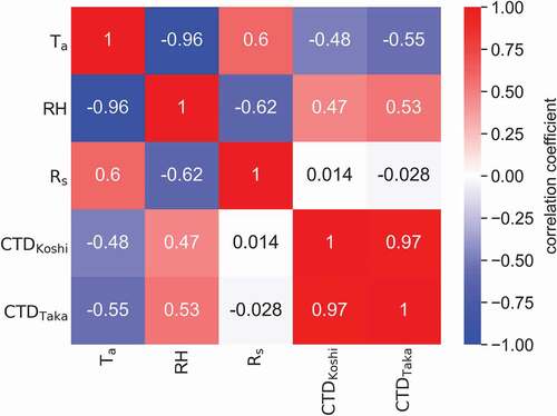
The correlation matrix calculated for the meteorological data and CTD is shown in Figure 4. This data revealed a strong negative correlation between T_a and RH (r = −0.96) and more moderate correlations between T_a and R_s (r = 0.60) and RH and R_s (r = −0.62). Of the three meteorological factors evaluated only CTD, T_a, and RH were moderately correlated with CTD in Koshihikari (r = −0.48, r = 0.47, respectively) and Takanari (r = −0.55, r = 0.53, respectively). In contrast, R_s was not correlated with CTD in either cultivar (r = 0.014 and r = −0.028, respectively).

Figure 4. The correlation coefficient matrix for the daytime air temperature (T_a), relative humidity (RH), solar radiation (R_s), and canopy temperature differences in Koshihikari (CTD_Koshi) and Takanari (CTD_Taka) cultivars. The color bar represents the value of the correlation coefficient.

Predicting canopy temperature differences

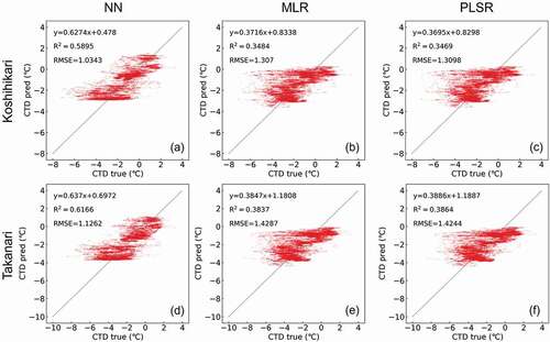
The results of CTD prediction for both the Koshihikari and Takanari using each of the three computational methods on 22 July 2017, and on 21 July 2018, are shown in Figures 5 and 6, respectively. On 22 July 2017, the prediction based on NN demonstrated the best accuracy (R² = 0.748, RMSE = 0.605°C, y = 0.787x + 0.280 in Koshihikari; R² = 0.7692, RMSE = 0.636°C, y = 0.770x + 0.062 in Takanari), while the other two methods presented with reduced accuracy (R² = 0.785, RMSE = 0.679°C, y = 0.662x + 0.622 in Koshihikari by MLR; R² = 0.785, RMSE = 0.684°C, y = 0.663x + 0.631 in Koshihikari by PLSR; R² = 0.726, RMSE = 0.715°C, y = 0.655x + 0.716 in Takanari by MLR; R² = 0.727, RMSE = 0.709°C, y = 0.653x + 0.699 in Takanari by PLSR). This trend was also observed for the predicted values for 21 July 2018, though the accuracies were lower than those for 2017 (R² = 0.348, RMSE = 1.307°C, y = 0.372x + 0.834 in Koshihikari by MLR, R² = 0.347, RMSE = 1.310°C, y = 0.370x + 0.830 in Koshihikari by PLSR, R² = 0.590, RMSE = 1.034°C, y = 0.627x + 0.478 in Koshihikari by NN, R² = 0.384, RMSE = 1.429°C, y = 0.385x + 1.180 in Takanari by MLR, R² = 0.386, RMSE = 1.424°C, y = 0.389x + 1.189 in Takanari by PLSR, and R² = 0.617, RMSE = 1.126°C, y = 0.637x + 0.697 in Takanari by NN). As mentioned above, these predictions were most accurate when calculated using the NN method. Therefore, the NN model was applied in the subsequent analyses.

Figure 5. Comparison of the observed values (CTD true) and predicted values (CTD pred) in Koshihikari (a) by neural network (NN), (b) by multiple linear regression (MLR), and (c) by partial least square regression (PLSR) and in Takanari (d) by NN, (e) by MLR, and (f) by PLSR, on 22 July 2017.

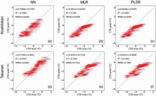
Figure 6. Comparison of the observed values (CTD true) and predicted values (CTD pred) in Koshihikari (a) by neural network (NN), (b) by multiple linear regression (MLR), and (c) by partial least square regression (PLSR) and in Takanari (d) by NN, (e) by MLR, and (f) by PLSR, on 21 July 2018.

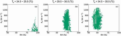
The differences in CTD between Takanari and Koshihikari (T_Taka – T_Koshi) under various meteorological conditions are shown in Figure 7. The RH, which is set on the x-axis, was restrained to 30% to 100%, while R_s was set on the y-axis and restrained to 0 W m⁻² to 1500 W m⁻². The T_a was set to 25°C, 30°C, and 35°C in Figure 7(a-c), respectively. The plots describing the observed weather conditions in response to a T_a between 24.5°C and 25.5°C, 29.5°C and 30.5°C, and 34.5°C and 35.5°C are shown in Figure 8(a-c), respectively. Figure 8 used the same x- and y-axes as Figure 7 to allow for direct comparisons. In Figure 7(a), CTD in Takanari was generally lower than Koshihikari when of RH was over 75% and R_s was under 900 W m⁻². A similar weather condition was wholly observed when T_a was from 24.5°C to 25.5°C (Figure 8(a)). When the T_a was set to 30°C, CTD in Takanari was generally lower than Koshihikari when the RH was over 60% and R_s under 1050 W m⁻², while the CTD for Koshihikari was generally lower than Takanari when RH was over 60% and R_s over 1050 W m⁻² (Figure 7(b)). However, both conditions could be observed when T_a was from 29.5°C to 30.5°C (Figure 8(b)). When T_a was set to 35°C, CTD was generally decreased in the Koshihikari variant compared to the Takanari cultivar when the RH was under 50% or over 75%, or R_s was under 900 W m⁻². However, the CTD in Koshihikari was higher than Takanari when RH ranged from 50% to 75% and R_s was over 900 W m⁻² (Figure 7(c)). Both conditions were also observed when T_a was from 34.5°C to 35.5°C (Figure 8(c)).

Figure 7. Heatmaps showing the varietal difference in the simulated values of canopy surface temperature in Koshihikari and Takanari (T_Taka – T_Koshi). In each panel, RH was retrained to between 30% and 100% and R_s was sequenced from 0 to 1500 W m⁻². The T_a was set to 25°C (a), 30°C (b), and 35°C (c). The color bar represents the T_Taka – T_Koshi values.

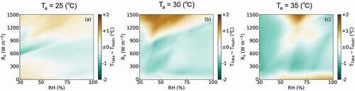
Figure 8. Plots describing the weather conditions observed over the course of the entire study. In each panel, RH was restrained between 30% and 100% and R_s was sequenced from 0 to 1500 W m⁻². The panels (a), (b), and (c) show the plots of each of these conditions in response to a T_a of between 24.5 and 25.5°C, 29.5 and 30.5°C, and 34.5 and 35.5°C, respectively.

Discussion

CTD was positively correlated with T_a and negatively correlated with RH (Figure 4), this is likely because higher temperatures are associated with lower RH and higher vapor pressure deficits (VPD), which induces higher latent heat flux, producing increased transpiration and reduced CTD. This result implies that the acceleration of transpiration by VPD exceeds the effect of stomatal closure, although a high VPD generally induces stomatal closure in most plants (Jalakas et al., 2021; Kimm et al., 2020; Ohsumi et al., 2008). R_s moderately correlates with T_a and higher R_s values are believed to contribute to greater transpiration, leading to higher T_a and photosynthetic rates. However, there was no direct correlation between R_s and CTD in our evaluations. The response of the stomata to sudden fluctuating light is relatively slow (Ohkubo et al., 2020; Sakoda et al., 2021; Tanaka et al., 2019; Taniyoshi et al., 2020), and this may have resulted in a time lag between light fluctuation and observable CTD. The difference between the R_s values recorded by the sensor and solar irradiation in the canopies may also have influenced.

The relationships between the observed and predicted CTD values based on MLR, PLSR, and NN modeling were much better than the direct correlation analyses estimating the relationships between various meteorological components and CTD (Figures 4–6). This is because T_c is more obviously affected by complex combinations of multiple meteorological components than single meteorological conditions, thus the application of large datasets accumulated over long periods allows a better understanding of these complex relationships. This means that our data models were better equipped to evaluate the relationships between CTD and specific weather conditions.

The predicted CTD values fit the observed values for 2017 and 2018 (Figures 5 and 6); however, the prediction accuracy on 21 July 2018, was lower than that on 22 July 2017. This is likely because 21 July 2018, produced CTD values ranging from −8 to 4°C, reducing the range of these values when compared to other studies, where the minimum CTD value was approximately −4°C (Fukuda et al., 2018; Zheng et al., 2020). It is worth noting that 21 July 2018, was extremely hot and dry, which may have led to a remarkably high VPD (Figure 3). This may have caused a considerable increase in the transpiration rate and thus a lower CTD (Figure 6), which could not be accurately predicted using any of the three computational methods described in this study. This may go some way to explaining the reduced accuracy for extremely low CTD values in this study, as these values fall outside of 94.8% of the total data sets, making these data points very rare (Figure 1(a)).

On 22 July 2017, and 21 July 2018, the slopes of the linear regression were closer to 1 in the prediction model created using NN than those produced using MLR and PLSR (Figures 5 and 6). In addition, the R² and RMSE values of the NN were better than those of the other two methods. The advantage of the NN model is its prediction range, where NN accommodated a CTD range of −4 to +2°C, while the MLR and PLSR models only supported a CTD range of −4 to 0°C. Because the majority of the CTD values over 0°C were observed under field conditions, it is thought that the NN prediction model is likely to be the best method for predicting CTD under these conditions. This is further supported by the fact that this NN model can predict CTD, an important indicator of crop growth and physiological condition, using only open-field scale meteorological data. The established NN model had better prediction accuracy within the CTD range from −4 to +2°C (Table S1), which covered 94.8% of all the observed data. Although the CTD prediction model in the present study is thought to be practical under most of weather conditions, further accumulation of data following extreme conditions (i.e. CTD under −4°C or over +2°C) are necessary to improve the robustness of our model.The simulated CTD values for the Takanari cultivar were generally lower than those of Koshihikari when R_s was under 900 W m⁻² (Figure 7), which was largely consistent with the observed data (Figure 8) and previous studies showing that the greater leaf photosynthetic capacity of Takanari is supported by high stomatal conductance and leaf nitrogen content (Hirasawa et al., 2010; Ohsumi et al., 2007a), stomatal density (Ohsumi et al., 2007b), hydraulic conductivity (Taylaran et al., 2011), and consequently, low leaf/canopy surface temperatures (Horie et al., 2006; Ikawa et al., 2017; Takai et al., 2010). However, the simulated CTD values for the Takanari cultivar were significantly increased when compared to the CTD values of Koshihikari when T_a was 30°C and R_s was over 1200 W m⁻² (Figure 7(b)) or when T_a was 35°C, RH was between 50% and 75%, and R_s was over 900 W m⁻² (Figure 7(c)). Many of these behaviors were confirmed in the observed data (Figure 8) and were largely consistent with the fact that reduced RH increases VPD. The simulated values on CTD in Koshihikari and Takanari under the same set of environments are shown in Figure S1.

Generally, the stomatal aperture in plants decrease under high VPD conditions (Inoue et al., 2021). A previous study reported that stomatal conductance decreased in Takanari when compared with Nipponbare, a typical japonica cultivar, under drought stress (Ohsumi et al., 2008). This is also supported by our previous observations that Takanari demonstrate a midday depression in leaf photosynthesis (Adachi et al., 2019a) and canopy transpiration (Kondo et al., 2021). Thus, the stomata of Takanari are thought to be more sensitive to extremely high VPD conditions than those of Koshihikari. Another possible reason for the reversal phenomenon may be the difference of aerodynamic characteristics in Koshihikari and Takanari. Takanari has larger leaf area, lower canopy height, and greater aerodynamic resistance under windless conditions (r_a*) than Koshihikari (Kondo et al., 2021). In other words, canopies of Takanari have structures that tend to prevent heat transfer to and from the atmosphere. In some cases of dry conditions, stomata of plants are closed, where the genotypic differences of photosynthetic traits were almost canceled. Under these conditions, the genotypic difference of heat diffusion attributed to canopy structures is thought to be a dominant factor affecting CTD. The reversal phenomenon was simulated under the conditions of R_s over 900 W m⁻² and T_a at 30°C, but not in T_a at 35°C (Figure 8). Further physiological research on Koshihikari and Takanari may be needed to reveal reasons for this inconsistency.

Despite the fact that our novel NN model enables fairly accurate prediction of CTD using only micrometeorological data, it remains limited in terms of genotypic and environmental diversity. This is because our model is specific to only two cultivars, both cultivated in Kyoto, Japan: Koshihikari and Takanari. One option to overcome this limitation is to extend the dataset by collecting CTD data for other cultivars and environments. However, collecting a comparable amount of data for new cultivars and environments is a time-consuming task. Another option for solving this problem is fine-tuning. In fine-tuning, we apply all the layers from the pre-trained NN model except for the last one and replace the final layer in the model with a new layer that has weights trained for its new targets. Previous studies have reported that the same level of prediction performance as full training can be achieved using a reduced dataset (Cetinic et al., 2018; Howard & Ruder, 2018; Tajbakhsh et al., 2016). Therefore, this technique may be useful in improving the versatility of this model moving forward.

Conclusion

Our NN model was able to predict CTD under field conditions using only meteorological data with practical accuracy under the conditions of CTD from −4°C to +2°C, covering 94.8% of all the observed data. This model accurately described the CTD values for Koshihikari and Takanari under moderate meteorological conditions and clearly modeled the varietal differences in response to specific environmental conditions. Thus, this newly established method may enable the evaluation of canopy gas exchange and its varietal characteristics in field-grown rice while reducing both labor and cost and expanding area of measurement with high time-resolution. Further collection of datasets under extreme conditions, in novel genotype, and at new location is needed to improve the versatility of this method.

Author contribution

Y.T. and R.K. established the experimental plan, R.K. conducted the experiments and wrote the manuscript, and all authors contributed extensively to its finalization.

Acknowledgments

This work was supported in part by the Japanese Society for the Promotion of Science (JSPS) KAKENHI under grant [numbers 19H02939, 20H02968, 21K19104, and 21H02172] (to Y.T.).

Disclosure statement

No potential conflict of interest was reported by the author(s).

Data Availability Statement

The data that support the findings of this study are available from the authors on reasonable request.

Supplementary material

Supplemental data for this article can be accessed online at https://doi.org/10.1080/1343943X.2022.2103003

References

- Adachi, S., Tanaka, Y., Miyagi, A., Kashima, M., Tezuka, A., Toya, Y., Kobayashi, S., Ohkubo, S., Shimizu, H., Kawai-Yamada, M., Sage, R. F., Nagano, A. J., & Yamori, W. (2019a). High-yielding rice Takanari has superior photosynthetic response to a commercial rice Koshihikari under fluctuating light. Journal of Experimental Botany, 70(19), 5287–5297. https://doi.org/10.1093/jxb/erz304
- Adachi, S., Yamamoto, T., Nakae, T., Yamashita, M., Uchida, M., & Karimata, R. (2019b). Genetic architecture of leaf photosynthesis in rice revealed by different types of reciprocal mapping populations. Journal of Experimental Botany, 70(19), 5131–5144. https://doi.org/10.1093/jxb/erz303
- Alberto, M. C. R., Wassmann, R., Buresh, R. J., Quilty, J. R., Correa, T. Q., Jr., Sandro, J. M., & Centeno, C. A. R. (2014). Measuring methane flux from irrigated rice fields by eddy covariance method using open-path gas analyzer. Field Crops Research, 160, 12–21. https://doi.org/10.1016/j.fcr.2014.02.008
- Anten, N. P. R. (1997). Modeling canopy photosynthesis using parameters determined from simple non-destructive measurements. Ecological Research, 12(1), 77–88. https://doi.org/10.1007/BF02523613
- Burkart, S., Manderscheid, R., & Weiglel, H. J. (2007). Design and performance of a portable gas exchange chamber system for CO2- and H2O-flux measurements in crop canopies. Environmental and Experimental Botany, 61(1), 25–34. https://doi.org/10.1016/j.envexpbot.2007.02.007
- Cetinic, E., Lipic, T., & Grgic, S. (2018). Fine-tuning convolutional neural networks for fine art classification. Expert Systems With Applications, 114, 107–118. https://doi.org/10.1016/j.eswa.2018.07.026
- Choudhury, B. J. (1987). Relationships between vegetation indices, radiation absorption, and net photosynthesis evaluated by a sensitivity analysis. Remote Sensing of Environment, 22(2), 209–233. https://doi.org/10.1016/0034-4257(87)90059-9
- Das, B., Nair, B., Reddy, V. K., & Venkatesh, P. (2018). Evaluation of multiple linear, neural network and penalised regression models for prediction of rice yield based on weather parameters for west coast of India. International Journal of Biometeorology, 62(10), 1809–1822. https://doi.org/10.1007/s00484-018-1583-6
- De Souza, A. P., Wang, Y., Orr, D. J., Carmo-Silva, E., & Long, S. P. (2020). Photosynthesis across African cassava germplasm is limited by Rubisco and mesophyll conductance at steady state, but by stomatal conductance in fluctuating light. New Phytologist, 225(6), 2498–2512. https://doi.org/10.1111/nph.16142
- Drake, B. G., & Leadley, P. W. (1991). Canopy photosynthesis of crops and native plant communities exposed to long-term elevated CO2. Plant, Cell & Environment, 14(8), 853–860. https://doi.org/10.1111/j.1365-3040.1991.tb01448.x
- Fan, J., Zheng, J., Wu, L., & Zhang, F. (2021). Estimation of daily maize transpiration rate using support vector machines, extreme gradient boosting, artificial and deep neural networks models. Agricultural Water Management, 245, 106547. https://doi.org/10.1016/j.agwat.2020.106547
- Fukuda, A., Kondo, K., Ikka, T., Takai, T., Tanabata, T., & Yamamoto, T. (2018). A novel QTL associated with rice canopy temperature difference affects stomatal conductance and leaf photosynthesis. Breeding Science, 68(3), 305–315. https://doi.org/10.1270/jsbbs.17129
- Gates, D. M. (1968). Transpiration and leaf temperature. Annual Review of Plant Physiology, 19(1), 211–238. https://doi.org/10.1146/annurev.pp.19.060168.001235
- Haghverdi, A., Washington-Allen, R. A., & Leib, B. G. (2018). Prediction of cotton lint yield from phenology crop indices using artificial neural networks. Computers and Electronics in Agriculture, 152, 186–197. https://doi.org/10.1016/j.compag.2018.07.021
- Hirasawa, T., Ozawa, S., Taylaran, R. D., & Ookawa, T. (2010). Varietal differences in photosynthetic rates in rice plants, with special reference to the nitrogen content of leaves. Plant Production Science, 13(1), 53–57. https://doi.org/10.1626/pps.13.53
- Horie, T., Matsuura, S., Takai, T., Kuwasaki, K., Ohsumi, A., & Shiraiwa, T. (2006). Genotypic difference in canopy diffusive conductance measured by a new remote-sensing method and its association with the difference in rice in rice yield potential. Plant, Cell & Environment, 29(4), 653–660. https://doi.org/10.1111/j.1365-3040.2005.01445.x
- Hou, M., Tian, F., Zhang, L., Li, S., Du, T., Huang, M., & Yuan, Y. (2019). Estimating crop transpiration of soybean under different irrigation treatments using thermal infrared remote sensing imagery. Agronomy, 9(1), 8. https://doi.org/10.3390/agronomy9010008
- Howard, J., & Ruder, S. (2018). Universal language model fine-tuning for test classification. arXiv:1801.06146v5. https://doi.org/10.48550/arXiv.1801.06146
- Ikawa, H., Chen, C. P., Sikma, M., Yoshimoto, M., Sakai, H., Tokida, T., Usui, Y., Nakamura, H., Ono, K., Maruyama, A., Watanabe, T., Kuwagata, T., & Hasegawa, T. (2017). Increasing canopy photosynthesis in rice can be achieved without a large increase in water use—A model based on free-air CO2 enrichment. Global Change Biology, 24, 1321–1341. https://doi.org/10.1111/gcb.13981
- Inoue, T., Sunaga, M., Ito, M., Yuchen, Q., Matsushima, Y., Sakoda, K., & Yamori, W. (2021). Minimizing VPD fluctuations maintains higher stomatal conductance and photosynthesis, resulting in improvement of plant growth in Lettuce. Frontiers in Plant Science, 12, 646144. https://doi.org/10.3389/fpls.2021.646144
- Jalakas, P., Takahashi, Y., Waadt, R., Schroeder, J. I., & Merilo, E. (2021). Molecular mechanisms of stomatal closure in response to rising vapour pressure deficit. New Phytologist, 232(2), 468–475. https://doi.org/10.1111/nph.17592
- Jin, X., Li, Z., Feng, H., Ren, Z., & Li, S. (2020). Deep neural network algorithm for estimating maize biomass based on simulated Sentinel 2A vegetation indices and leaf area index. The Crop Journal, 8(1), 87–97. https://doi.org/10.1016/j.cj.2019.06.005
- Johnson, I. R., & Thornley, J. H. (1984). A model of instantaneous and daily canopy photosynthesis. Journal of Theoretical Biology, 107(4), 531–545. https://doi.org/10.1016/S0022-5193(84)80131-9
- Jones, H. G. (2014). Plants and microclimate (3rd ed.) Cambridge University Press.
- Jones, H. G., Hutchinson, P. A., May, T., Jamali, H., & Deery, D. M. (2018). A practical method using a network of fixed infrared sensors for estimating crop canopy conductance and evaporation rate. Biosystems Engineering, 165, 59–69. https://doi.org/10.1016/j.biosystemseng.2017.09.012
- Katsura, K., Maeda, S., Horie, T., & Shiraiwa, T. (2006). A multichannel automated chamber system for continuous measurement of carbon exchange rate of rice canopy. Plant Production Science, 9(2), 152–155. https://doi.org/10.1626/pps.9.152
- Kimm, H., Guan, K., Gentine, P., Wu, J., Bernacchi, C. J., Sulman, B. N., Griffis, T. J., & Lin, C. (2020). Redefining droughts for the U.S. corn belt: The dominant role of atmospheric vapor pressure deficit over soil moisture in regulating stomatal behavior of maize and soybean. Agricultural and Forest Meteorology, 287, 107930. https://doi.org/10.1016/j.agrformet.2020.107930
- Kondo, R., Tanaka, Y., Katayama, H., Homma, K., & Shiraiwa, T. (2021). Continuous estimation of rice (Oryza Sativa (L.)) canopy transpiration realized by modifying the heat balance model. Biosystems Engineering, 204, 294–303. https://doi.org/10.1016/j.biosystemseng.2021.01.016
- Li, S., Fleisher, D. H., Wang, Z., Barnaby, J., Timlin, D., & Reddy, V. R. (2021). Application of a coupled model of photosynthesis, stomatal conductance and transpiration for rice leaves and canopy. Computers and Electronics in Agriculture, 182, 106047. https://doi.org/10.1016/j.compag.2021.106047
- Long, S. P., Zhu, X. G., Naidu, S. L., & Ort, D. R. (2006). Can improvement in photosynthesis increase crop yields? Plant, Cell & Environment, 29(3), 315–330. https://doi.org/10.1111/j.1365-3040.2005.01493.x
- Ma, J., Li, Y., Chen, Y., Du, K., Zheng, F., Zhang, L., & Sun, Z. (2019). Estimating above ground biomass of winter wheat at early growth stages using digital images and deep convolutional neural network. European Journal of Agronomy, 103, 117–129. https://doi.org/10.1016/j.eja.2018.12.004
- Monsi, M., & Saeki, T. (2005). On the factor light in plant communities and its importance for matter production. Annals of Botany, 95(3), 549–567. https://doi.org/10.1093/aob/mci052
- Monteith, J. L. (1995). A reinterpretation of stomatal response to humidity. Plant, Cell & Environment, 18(4), 357–364. https://doi.org/10.1111/j.1365-3040.1995.tb00371.x
- Monteith, J. L., & Unsworth, M. H. (2013). Principles of environmental physics (4th ed.) ed.). Academic Press.
- Morison, J. I. L., & Gifford, R. M. (1983). Stomatal sensitivity to carbon dioxide and humidity. Plant Physiology, 71(4), 789–796. https://doi.org/10.1104/pp.71.4.789
- Mujahidin, S., Azhar, N. F., & Prihasto, B. (2021). Analysis of using regularization technique in the convolutional neural network architecture to predict paddy disease for small dataset. Journal of Physics: Conference Series, 1726, 012010.
- Nam, D. S., Moon, T., Lee, J. W., & Son, J. E. (2019). Estimating transpiration rates of hydroponically-grown paprika via an artificial neural network using aerial and root-zone environments and growth factors in greenhouses. Horticulture, Environment, and Biotechnology, 60(6), 913–923. https://doi.org/10.1007/s13580-019-00183-z
- Nevavuori, P., Narra, N., & Lipping, T. (2019). Crop yield prediction with deep convolutional neural networks. Computers and Electronics in Agriculture, 163, 104859. https://doi.org/10.1016/j.compag.2019.104859
- Ohkubo, S., Tanaka, Y., Yamori, W., & Adachi, S. (2020). Rice cultivar Takanari has higher photosynthetic performance under fluctuating light than Koshihikari, especially under limited nitrogen supply and elevated CO2. Frontiers in Plant Science, 11, 1308. https://doi.org/10.3389/fpls.2020.01308
- Ohsumi, A., Hamasaki, A., Nakagawa, H., Yoshida, H., Shiraiwa, T., & Horie, T. (2007a). A model explaining genotypic and ontogenetic variation of leaf photosynthetic rate in rice (Oryza Sativa) based on leaf nitrogen content and stomatal conductance. Annals of Botany, 99(2), 265–273. https://doi.org/10.1093/aob/mcl253
- Ohsumi, A., Kanemura, T., Homma, K., Horie, T., & Shiraiwa, T. (2007b). Genotypic variation of stomatal conductance in relation to stomatal density and length in rice (Oryza Sativa L.). Plant Production Science, 10(3), 323–328. https://doi.org/10.1626/pps.10.322
- Ohsumi, A., Hamasaki, A., Nakagawa, H., Homma, K., Horie, T., & Shiraiwa, T. (2008). Response of leaf photosynthesis to vapor pressure difference in rice (Oryza sativa L) varieties in relation to stomatal and leaf internal conductance. Plant Production Science, 11(2), 184–191. https://doi.org/10.1626/pps.11.184
- Ohtaki, E. (1984). Application of an infrared carbon dioxide and humidity instrument to studies of turbulent transport. Boundary-Layer Meteorology, 29(1), 85–107. https://doi.org/10.1007/BF00119121
- Qu, M., Hamdani, S., Li, W., Wang, S., Tang, J., Chen, Z., song, Q., Li, M., Zhao, H., Chang, T., Chu, C., & Zhu, X. G. (2016). Rapid stomatal response to fluctuating light: An under-explored mechanism to improve drought tolerance in rice. Functional Plant Biology, 43(8), 727–738. https://doi.org/10.1071/FP15348
- Sakoda, K., Taniyoshi, K., Yamori, W., & Tanaka, Y. (2021). Drought stress reduces crop carbon gain due to delayed photosynthetic induction under fluctuating light conditions. Physiologia Plantarum, 174(1), e13603. https://doi.org/10.1111/ppl.13603
- Salter, W. T., Merchant, A. M., Richards, R. A., Trethowan, R., & Buckley, T. N. (2019). Rate of photosynthetic induction in fluctuating light varies widely among genotypes of wheat. Journal of Experimental Botany, 70(10), 2787–2796. https://doi.org/10.1093/jxb/erz100
- Soleh, M. A., Tanaka, Y., Nomoto, Y., Iwahashi, Y., Nakashima, K., Fukuda, Y., Long, S. P., & Shiraiwa, T. (2016). Factors underlying genotypic differences in the induction of photosynthesis in soybean [Glycine max (L.) Merr.]. Plant, Cell & Environment, 39(3), 685–693. https://doi.org/10.1111/pce.12674
- Song, Q., Xiao, H., Xiao, X., & Zhu, X. G. (2016). A new canopy photosynthesis and transpiration measurement system (CAPTS) for canopy gas exchange research. Agricultural and Forest Meteorology, 217, 101–107. https://doi.org/10.1016/j.agrformet.2015.11.020
- Tajbakhsh, N., Shin, J. Y., Gurudu, S. R., Hurst, R. T., Kendall, C. B., Gotway, M. B., & Liang, J. (2016). Convolutional neural networks for medical image analysis: Full training or fine tuning? IEEE Transactions on Medical Imaging, 35(5), 1299–1312. https://doi.org/10.1109/TMI.2016.2535302
- Takai, T., Yano, M., & Yamamoto, T. (2010). Canopy temperature on clear and cloudy days can be used to estimate varietal differences in stomatal conductance in rice. Field Crops Research, 115(2), 165–170. https://doi.org/10.1016/j.fcr.2009.10.019
- Tanaka, Y., Adachi, S., & Yamori, W. (2019). Natural genetic variation of the photosynthetic induction response to fluctuating light environment. Current Opinion in Plant Biology, 49, 52–59. https://doi.org/10.1016/j.pbi.2019.04.010
- Tanaka, Y., Watanabe, T., Katsura, K., Tsujimoto, Y., Takai, T., Tanaka, T., Kawamura, K., Saito, H., Homma, K., Mairoua, S., Ahouanton, K., Ibrahim, A., Senthilkumar, K., Semwal, V., Matute, E., Corredor, E., El-Namaky, R., Manigbas, N., Quilang, E., & Saito, K. (2021). Deep learning-based estimation of rice yield using RGB image. Research Square. https://doi.org/10.21203/rs.3.rs-1026695/v1
- Taniyoshi, K., Tanaka, Y., & Shiraiwa, T. (2020). Genetic variation in the photosynthetic induction response in rice (Oryza sativa L.). Plant Production Science, 23(4), 513–521. https://doi.org/10.1080/1343943X.2020.1777878
- Taylaran, R. D., Adachi, S., Ookawa, T., Usuda, H., & Hirasawa, T. (2011). Hydraulic conductance as well as nitrogen accumulation plays a role in the higher rate of leaf photosynthesis of the most productive variety of rice in Japan. Journal of Experimental Botany, 62(11), 4067–4077. https://doi.org/10.1093/jxb/err126
- Taylor, S. H., & Long, S. P. (2017). Slow induction of photosynthesis on shade to sun transitions in wheat may cost at least 21% of productivity. Philosophical Transactions of the Royal Society B: Biological Sciences, 372(1730), 20160543. https://doi.org/10.1098/rstb.2016.0543
- Van Rossum, G., & Drake, F. L. (2009). Python 3 reference manual. Create Space: Scotts.
- Wu, A., Hammer, G. L., Farquhar, G. D., & Farquhar, G. D. (2019). Quantifying impacts of enhancing photosynthesis on crop yield. Nature Plants, 5(4), 380–388. https://doi.org/10.1038/s41477-019-0398-8
- Yamori, W., Hirosaka, K., & Way, D. A. (2014). Temperature response of photosynthesis in C3, C4, and CAM plants: Temperature acclimation and temperature adaption. Photosynthesis Research, 119(1–2), 101–117. https://doi.org/10.1007/s11120-013-9874-6
- Yamori, W., Kusumi, K., Iba, K., & Terashima, I. (2020). Increased stomatal conductance induces rapid changes to photosynthetic rate in response to naturally fluctuating light conditions in rice. Plant, Cell & Environment, 43(5), 1230–1240. https://doi.org/10.1111/pce.13725
- Yoon, D. K., Ishiyama, K., Suganami, M., Tazoe, Y., Watanabe, M., Imaruoka, S., Ogura, M., Ishida, H., Suzuki, Y., Obara, M., Mae, T., & Makino, A. (2020). Transgenic rice overproducing Rubisco exhibits increased yields with improved nitrogen-use efficiency in an experimental paddy field. Nature Food, 1(2), 134–139. https://doi.org/10.1038/s43016-020-0033-x
- Zheng, E., Zhang, C., Qi, Z., & Zhang, Z. (2020). Canopy temperature response to the paddy water content and its relationship with fluorescence parameters and dry biomass. Agricultural Research, 9(4), 599–608. https://doi.org/10.1007/s40003-019-00452-4
- Zhu, X. G., Long, S. P., & Ort, D. R. (2010). Improving photosynthetic efficiency for greater yield. Annual Review of Plant Biology, 61(1), 235–261. https://doi.org/10.1146/annurev-arplant-042809-112206