Multi-scale analysis of residential behaviour based on UWB indoor positioning system-a case study of retired household in Beijing, China

ABSTRACT

This paper proposes a data acquisition and analysis workflow and framework to clarify the daily residential behaviour of occupants based on the UWB indoor positioning system. The daily activities are analysed in different scales, namely grid level, convex polygon level and room level. At the first level, how long occupants stay in each 1 m*1 m grid was calculated, so that areas occupants stay longer was obtained. In the convex polygon level, the structure of the spatial network was clarified through analysis of the properties of each zone and weight of their connections. Although the network dynamically changes when the users and time differ, general patterns can be captured through analysis of large amounts of data. In the room level, which is the common analysing units, we get the movements between rooms and analysed the room-based behavioural networks of family members. Based on the findings in three levels, new variables were introduced in a regression model, and mutual visibility is found to significantly affect the household’s behaviour. By introducing the high-resolution indoor positioning system and the network analysis most used in the urban and social studies, this research provides a new prospect of data collecting and analysis of occupant indoor behaviour.

KEYWORDS:

• Residential behaviour
• UWB indoor positioning system
• convex polygon
• network analysis
• spatial-temporal data

1. Introduction

Residential houses are spaces where people spend most of their time, especially for the elderly. People’s living habits are constantly changing, whereas we are not very clear about that how do people use the residential house and what are their real needs for the dwelling. Therefore, the home design usually cannot match well with the user’s requirements. The utilisation of houses can be improved by analysing the living behaviours of the household, while traditional methods including questionnaire survey and interview cannot depict the whole picture of the problem. With the emergence of big data science, behaviour data acquisition method has been developed from traditional ways of observation to real-time and high-resolution positioning technology, which is non-invasive and objective. Many previous researchers have explored built-up environmental physical factors affecting household satisfaction, however, seldom have they focused on the relationship between the occupants’ activity and spatial configuration of the house using spatial-time data. Also, there is no perfect research framework for how to apply these data, especially in the analysis of the interior space of buildings.

With the new method of behaviour data collection based on UWB indoor positioning technology, this study attempts to present a research workflow from data collection, analysis and visualisation, to statistics in the form of a case study, in order to explore the relationship of residential use and house layout. To be more specific, it aims to make clear the daily activities and movements of the occupants and visualise the spatial networks of the occupants. Moreover, by partitioning the space into multi-levels, that is in grid level, convex polygon level and room level, this research more accurately reveals the actual state of affairs of daily use. Finally, inspired by some of the basic phenomena and laws derived from the aforementioned analysis, we can further analyse the factors affecting their behaviour.

2. Previous studies

2.1. Post-occupancy evaluation of the residential house

Post-occupancy evaluation (POE) is defined as an examination of the effectiveness for human users of occupied, designed environments (Zimring and Reizenstein 1980). POE has been applied in projects of different types of living houses, dormitories to hospitals, commercials and even urban environment. Preiser, White, and Rabinowitz (2015) provided systematic guidance on the evaluation of buildings in use for designers to learn lessons from successful and unsuccessful building performance. On residential field, many researchers focused on the post-use satisfaction survey of green buildings, and some scholars had built a post-use evaluation index system for the household satisfaction (Kyu-in and Dong-woo 2011; Phillips et al. 2004). Ibem et al. (2013) focused on the design and construction aspects, and assessed the performance of residential buildings based on user satisfaction surveys. They found the satisfaction level with privacy in the buildings was higher than other aspects of the buildings and the most important factor determining satisfaction was the type, location and aesthetic appearance of the buildings. The post-occupancy evaluation has become more precise with the big data science, and the object has also moved from the measurement of the built-in environmental physical quantity to the measurement of the user’s subjective psychological quantity.

However, these studies based on satisfaction survey or self-reported data cannot measure the occupants’ indoor behaviour precisely for the reason that asking people to recall or record their long-hour activity in detail is tiresome and boring. Therefore, we are in need of a better way to record people’s in-depth movements continuously over a long period of time.

2.2. Behavioural data acquisition method

Behavioural observation is the most common method used to investigate people’s behaviour in associated environments (Yun et al. 2003). It has been applied in collecting children’s behaviour in the residential landscape (Zeng and Li 2018), and also in recording the resident’s day-to-day behaviour in a nursing organisation (Hsieh 2010). Based on behavioural observation, behaviour mapping is a visual observation method that uses different types of points to represent various physical activity behaviours (Cosco, Moore, and Islam 2010).

New sensing and communication technology has been brought to the field of capturing human behaviour and positioning information. At MIT, a multi-disciplinary team (Intille 2002) was developing technologies and design strategies for the future home, the ubiquitous sensing such as image-based experience sampling and reflection was used to study human behaviour at home quantitatively and qualitatively. Ozturk, Arayici, and Coates (2012) used wireless remote sensors to collect environmental data and augment BIM models, thus realise real-time post-occupancy evaluation. Qu et al. (2010) used RFID technology to analyse the movements and main links between dwelling units of Chinese elderly couples. Zhang et al. (2011) clarified how workers stay in a place and move differently in territorial and non-territorial workplaces by using the UWB (Ultra Wide Band impulse radio) sensor network.

There is still a research gap between the data acquisition method and the research objective. Using camera to collect behaviour data may infringe on the privacy of family members, thereby it is constrained only in the laboratory scenes and is not acceptable for recording family members’ private daily life. The RFID method does not involve privacy issues, however, being limited to the low positioning accuracy and poor anti-interference performance, it could only support analysis on room-level. Comparing to RFID and other positioning technology, UWB has higher spatial and temporal resolution and better stability, thus this method can record the behaviour in much finer grained scale such as furniture-level and grid-level.

2.3. Spatial analysis method

Space syntax, pioneered in the 1970s by Prof Bill Hillier, investigates the relationship between the spatial configuration and human societies (Hillier et al. 1976). The convex map is the most popular means of describing the spatial configuration of building plans. Instead of discrete units separated following the preset wall boundaries straightforwardly, partitioning the given layout into convex polygons can capture the actual characteristics of the spatial structure (Bafna 2003).

With the generation of multi-source data, network analysis based on big data has been developed to clarify the spatial configuration and widely used in urban-related research. Network refers to the concept constructed by nodes and edges to reflect the relationship between different objects or elements. The in-degree refers to the popularity of a certain node and the out-degree indicates the expansiveness of a certain node. Centrality is used to express the degree to which a point is located in the centre of the entire network (Scott 2017). De Montis et al. (2007) used a weighted network representation in which vertices correspond to towns and the edges correspond to the actual commuting flows among those towns, and shed light on several structural and organisational properties of the inter-municipal traffic system. Reades, Calabrese, and Ratti (2009) conducted large-scale interurban research using the mobile phone network and helped understand the eigenspace and the dynamic flows between cities.

Few studies have linked the spatial configuration with real-world behaviour data to analyse that how spatial features affect human behaviour. This paper intends to reveal some behavioural patterns and explain them using the spatial syntax and network theories, and to construct a more complete analytical framework.

3. Material and methodology

3.1. Equipment composition and principle

The UWB device has the lowest nominal TX power (−41.3 DBm/MHz) among all the indoor positioning systems, which is a great advantage of a portable device since it needs to transfer large information at a relatively low cost of energy. Due to the wideband and high pulse rate property of UWB devices, UWB Real Time Locating System (RTLS) can easily limit its accuracy to 10–30 cm using time of arrival (TOA) and trilateration positioning algorithm.

The UWB system consists of tags, anchors, terminal server and database (Figure 1). Tags will be disputed to the participants to get their trajectories. These tags will send messages to nearby anchors at a rate of once per second. Then anchors will send those messages to the server through the wireless network. We also developed a RTLsoftware to analyse those messages and display tags’ real-time location on the interface.

Figure 1. (1) Configuration of UWB system; (2) Interface of RTLsoftware.

3.2. Outline of investigation

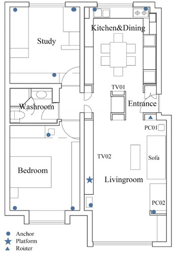
Compared with young people who go to work during the day, older people spend more time at home and have more demand for housing. This research chose a pair of retired professors in their 70 s who were in good physical condition and had a regular life. Their residence was located on the 3rd floor with elevators in a residential area in Haidian District, Beijing (Table 1). The housing units included one bedroom, study room, living room, kitchen and bathroom, with a total area about 77 m². The dining room shared space with the kitchen, which was separated from the living room by a cabinet. There was a TV both in the kitchen and living room, and a computer on each side of the sofa in the living room.

Table 1. Outline of the investigated.

Member	Retired couple
Age	Husband: 70+ Wife: 70+
Job	Husband: Professor Wife: Professor
Type	2LBK
Area	77 m^2
Location	Haidian District, Beijing
Floor	3rd
Elevator	Available
Investigation period	3 weeks

3.3. Experiment progress

3.3.1. Installation

In preparation for the installation, we mapped the house and furniture, established a Cartesian coordinate system based on the appropriate origin on the plane, and determined the position of the tag according to the house plan and furniture placement. Then we installed 3 anchors in each room, with each anchor installed approximately 2 meters above the ground on the wall to ensure it covered the entire room. Routers and the computer were placed close to the centre of the house and remained working during the experiment. Tags with unique ID were disputed to family members. After the installation was completed, we set up the computer platform, connected it to the local route, and input the spatial location information of the floor plan and anchors. During the experiment, the coordinates of the tags were calculated and stored in the database. Figure 2 shows the detail of the equipment arrangement.

Figure 2. House plan and equipment arrangement.

3.3.2. Monitor

Before the investigation began, the couple were informed of the use of the tags and charging requirement, and also received a daily life record sheet to record their sleep time, time out and tag charging time. The study lasted for 3 weeks and the equipment was withdrawn at the end of the experiment to restore the original condition of the house. Thereafter, we conducted a short interview with the couple on the basis of the collected data.

3.4. Data pre-processing

We preprocessed the experimental raw data stored on the server including the subject ID, time, and coordinate information. Firstly, we removed the anomaly data due to device instability and signal reflections. Secondly, the original data was proofread and missing values were filled. According to the questionnaire survey and life record table, the raw data hollowed out during the nap and outing time were filled. Then, the house plan was partitioned into different units, according to different scales, and the location information was converted to the corresponding unit label. The preprocessed database is shown in Table 2.

Table 2. Preprocessed database.

Date	Subject ID	X	Y	Grid ID	Zone ID	Room
2017-12-16 20:52:44	1	7.143719	2.6577	78	9	Livingroom
2017-12-16 20:52:54	2	6.3816	2.1309	77	22	Livingroom
2017-12-16 20:52:59	1	6.6638	1.1959	87	10	Balcony
2017-12-16 20:53:03	2	6.8903	2.4709	77	10	Balcony

4. Data analysis method and result

4.1. Occurrence frequency distribution in 1 m*1 m grid scale

At the beginning of the analysis, we wanted to visualise the regularity of the x-y position points generated by tags of family members, and to conduct further analysis on this basis. Instead of using the kernel density method of processing continuous x-y position points, we adopted the grid aggregation method to convert continuous x-y point data into discrete grids. Grids were numbered sequentially, and their values were calculated, compared and sorted. Grid aggregation is a method of fine-grained, small-scale analysis of human behaviour. This method meshes planes and maps position information to corresponding grid. As for the size of the grid, it was due to the personal distance, which “might be thought as a small protective sphere or bubble that an organism maintains between itself and others” (Hall 1910), is about 0.76–1.2 m, hence we standardise the unit to an integer 1 meter (Figure 3).

Figure 3. Grid plan.

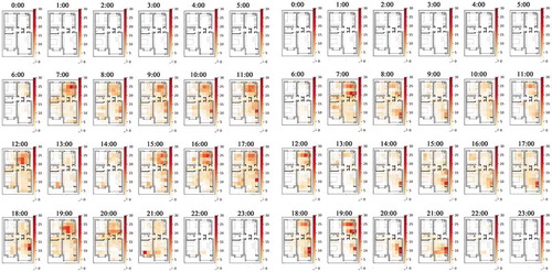
As the position data was evenly produced by time, by calculating the amount of data falling into each grid over a period of time, the length of time that occupants stayed on each grid during this period was obtained. Figure 4 shows the length of time each family member stayed at different locations in the house every hour. The longer they stayed, the darker the colour of the grid. It can be seen that they usually got up at about 7:00 in the morning and fell asleep at about 10 o’clock in the evening, and had a lunch break between 13:00 and 15:00. The couple were active in the kitchen stove area in the morning. During the rest of the day, the occurrence frequency in the dining table area (watching TV) was high for the host, and it was high for the hostess in the living room around sofa and computer.

Figure 4. 24-hour heat map of occurrence: (1) host; (2) hostess.

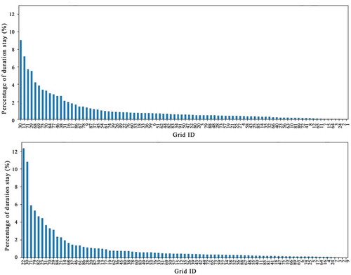
The sum of the couple’s stay time in each grid in two weeks was counted, and the ratio was calculated to obtain Figure 5. The abscissa is the grid ID and the ordinate is the proportion of time spent on this grid. It can be seen that during the daytime, except for the nap time and the outing time, in more than 75% of the space (about 55 m²), the length of stay of the couple is less than 1% of the daytime (less than 10 min). The space with a stay time ratio of more than 5% (more than half an hour) accounts for about 5% of the total area (about 4 m²). The grid ID with the longest stay of the husband was 30, and 22 for the wife, including the time they spent together.

Figure 5. Statistic of stay time in each grid: (1) host; (2) hostess.

4.2. Network analysis of zones

Although the grid aggregation method is more refined and simpler to operate, it has some limitations, such as the grid has no real entity meaning. The indoor activities of people are closely related to the position of the furniture, so it is more conducive to partition the plane into different zones according to the furniture arrangement. Each plane may have several ways of division. After several attempts, this study followed the principle of convex polygon mentioned above (Bafna 2003), and divided the plane into 36 convex polygons numbered 0–35 (Figure 6).

Figure 6. Zone plan of convex polygons.

Based on the convex polygons and human movements, the spatial networks are formed. 36 convex polygons constitute the nodes of networks, and the family members’ movements between the polygons form the edge elements of their own network. It is worth mentioning that, in this study, the edge between convex polygons does not exist only between two adjacent convex polygons, but also between the origin zone and the destination zone of occupants’ movements. For example, when a person went from origin zone A to destination zone C through zone B, then there are connections between A and B, B and C, A and C, wherein the OD space and the passing space are distinguished by the length of the staying time.

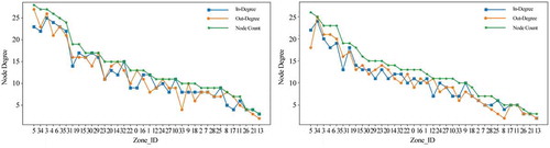
Since entering a room and leaving a room are two activities, the occupant’s behavioural network can be regarded as a directed graph. Figure 7 shows the attributes of each node in the behavioural network of different family members. In-degree represents the number of other nodes that reach the current node. Conversely, out-degree represents the number of other nodes arrived from the current node. The node-count represents the number of other nodes associated with the current node, which is the union of in-degree and out-degree. The five nodes with the highest degree for the host are 5, 31, 34, 4, and 3 in sequence, and it is 5,34,3,4,6 for the hostess.

Figure 7. Node property distribution: (1) host; (2) hostess.

Figure 8 shows the behavioural network diagram of two people in the morning, afternoon, and evening. The node size in the figure represents the sum of the frequency a person entered the zone and left the zone, and the line width represents the strength of the connection between nodes. In terms of connection strength, the host had a high frequency of entering and leaving the cooking zone (zone 0) and dining table zone (zone 3) during the day. The hostess had a high-frequency shuttle between the cooking zone (zone 0) and dining table zone (zone 3) in the morning, and connection between the sofa (zone 8) and computer desk area (zone 9) of the living room was high in the afternoon. In terms of the structure of connections, the network of the host in the morning was more complicated, while it was more complicated in the afternoon for the hostess. It indicates that the couple was active in different period of the day.

Figure 8. Movements networks between zones: (1) host in the morning, afternoon, night; (2) hostess in the morning, afternoon, night.

Based on the data of three weeks, a comprehensive network diagram of the behaviour of the two occupants can be obtained. In Figure 9, the digits are the IDs of the convex polygons consist with the foregoing, the node size indicates the eigenvector centrality, which quantises the influence of the node in the network, and the line width is determined by the movement frequency. The nodes with the largest eigenvector centrality will locate in the middle of the figure, and points with a high frequency of connections are gathered together. Comparing the two network diagrams, there is only one obvious group of nodes with both high centrality and connection frequency in the network of the hostess, which is 8-11-12, while three groups can be seen in the host’ network, namely 0-1-2-3-23, 8-11-12, and 5-13-14. It can be inferred that the host was used to walking around while the hostess was likely to stay in one place for long.

Figure 9. Zone network structure: (1) host; (2) hostess.

4.3. Movements between rooms

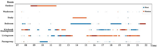
We adopted the network analysis approach to analyse the room-based behavioural networks of occupants. In this study, the plane was divided into 8 parts that are consistent with the room units. The behaviour network is a dynamic network that changes over time. Figure 10 shows the networks of the couple’s movements between rooms in the morning (7:00–12:00), afternoon (12:00–18:00) and night (18:00–24:00) of the day. Generally, the three strongest connections lie between the kitchen and living room, living room and bedroom, as well as bedroom and bathroom. Subtle differences existed in the couple’s networks at different period of time. For example, their main nodes were different as it was the kitchen for the host and living room for the hostess.

Figure 10. Movements networks between rooms: (1) host in the morning, afternoon, night; (2) hostess in the morning, afternoon, night.

To get more detailed information, we got a time series table showing the occupants’ movements and which room they were in at each moment during the investigation. In a typical day (Figure 11), two elderly people usually went out in the morning, and during the lunch break, the couple had a rest in the bedroom and study respectively. Table 4 is the information obtained through interviews. In comparison, the information obtained by IPS is more comprehensive, detailed and non-invasive. For example, we can get the location of their specific activities continuously.

Table 3. Daily activity information from the interview.

	Sat.	Sun.	Mon.	Tue.	Wed.	Thu.	Fri.
6:30–8:30	breakfast
8:30–12:00	40min walk outside			hospital cultural activities		market;(host); cultural activities(hostess)	40min walk outside
12:30–13:00	lunch
13:00–15:00	snap； charge the tag
16:00–17:00						shower
19:00–20:00	dinner
20:00–21:00	watch TV at dining room(host)； watch TV at livingroom(hostess)；
22:00–06:30	go to bed；charge the tag

Table 4. Lasso coefficient of the model of the host.

(Intercept)	Visual_Integration_HH	VisualMeanDepth	VisualRelativisedEntropy	VisualStepDepth_sf
7.439736924	0.000000000	−0.153205997	−0.436378909	−0.259613775
Control	Choice	Mean_Depth	dist_door	dist_windo
0.005043898	0.000000000	0.000000000	−0.201465981	0.000000000
Room_balcony	Room_bedroom	Room_toilet	Room_ livingroom	Room_diningroom
0.000000000	−0.189543046	0.000000000	0.100915161	0.374978667
Zone_furniture	Zone_sittingarea
0.000000000	−0.502297449

Figure 11. Time series table.

4.4. Regression

Based on the above analysis, the stay time of the couple in each grid was acquired, then the multiple regression model was applied to explore the factors affecting stay time in different space. Preliminary assumptions about the influencing factors may include:

1） Room type, zone type, distance to windows and doors.

1. Roomtype：Each grid is assigned a value of the type of room in which each grid is located, room types are classified into the aisle (reference), living room, dining room, bedroom, toilet, balcony.

2. Zonetype：Zone types are classified into the aisle(reference), sitting area, furniture, and are assigned to the grid according to their location.

3. Dist_window: Indicates the distance of each grid to the window, which is roughly used to measure the impact of sunshine.

4. Dist_door: Calculate the distance of each grid to the door and roughly measure the depth level of each grid in the room.

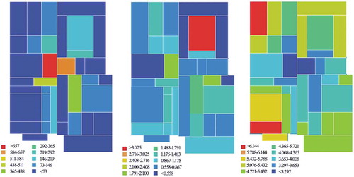
2） The visual analysis based on 0.1 m*0.1 m grid and space depth analysis based on zones. Visual_Integration_HH, VisualMeanDepth, VisualRelativisedEntropy measures the extent to which the spaces are mutually visible (Figure 12). Choice, Control, Mean Depth measures the accessibility of space (Figure 13).

Figure 12. (1) Visual_Integration_HH; (2) Visual mean depth; (3) VisualRelativisedEntropy.

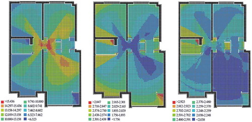
Figure 13. (1) Choice; (2) Control; (3) Mean Depth.

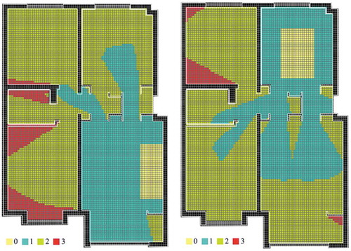
3） Local visibility analysis. We noticed the couple often stayed in spaces where they could see each other. The host liked staying near the dining table, and the hostess liked staying near the sofa. Therefore, when analysing factors affecting the stay time of the host, the visual step depth from the sofa is taken into consideration, and the same when analysing the hostess’ behaviour.

1. Visual step depth_sf (Figure 14(1)): Visual step depth from the sofa.

2. Visual step depth_dt (Figure 14(2)): Visual step depth from the dinner table.

   Figure 14. (1) Visual step depth_sf; (2) Visual step depth_dt.

   

After the above data was calculated, each grid was used as a statistical unit for regression analysis. There may exist high correlations between the independent variables, so the lasso regression method was applied, which can avoid the multicollinearity between the variables and can also select the variables, as well as to achieve the optimal balance between the variance and the deviation of the model.

Standard multiple linear regression equation is:

$\mathrm{y}={\beta }_0+{\beta }_1{\chi }_1+\dots +{\beta }_{\rho }{\chi }_{\rho }+\epsilon$

Where the dependent variable y is the stay time in each grid, and it is normally distributed by log transformation.

The coefficient ${\hat{\beta }}_{L\mathrm{a}\mathrm{s}\mathrm{s}\mathrm{o}}$ of the lasso is obtained by solving the following formula：

${\hat{\beta }}_{L\mathrm{a}\mathrm{s}\mathrm{s}\mathrm{o}}=ar{g}_{\beta }min\left(\sum _{i=1}^n{\left(y_i-{\beta }_0-\sum _{j=1}^p{\beta }_j{\chi }_{ij}\right)}^2+\lambda \sum _{j=1}^p\left|{\beta }_j\right|\right)$

Where $\lambda {\sum }_{j=1}^p\left|{\beta }_j\right|$ is the penalty term for the model coefficients, and $\lambda$ was determined using the cross-validation method, when the test set reached the minimum MSE (Mean Squared Error).

The initial full model was established for the host and the hostess respectively, and the variables in two models were the same except for the Visual Step Depth. The regression results are as Table 4 and Table 5 show.

Table 5. Lasso coefficient of the model of the hostess.

(Intercept)	Visual_Integration_HH	VisualMeanDepth	VisualRelativisedEntropy	VisualStepDepth_dt
6.64288725	0.01667651	0.000000000	0.000000000	−0.57728492
Control	Choice	Mean_Depth	dist_door	dist_windo
0.005043898	0.000000000	−0.23038715	−0.09620982	0.000000000
Room_balcony	Room_bedroom	Room_toilet	Room_ livingroom	Room_diningroom
0.000000000	−0.31710061	0.000000000	0.34573755	0.77182997
Zone_furniture	Zone_sittingarea
−0.05378028	0.000000000

The regression model for the host is:

$\begin{array}{rl}& \mathrm{y}=7.44-0.15\times [\mathrm{V}\mathrm{i}\mathrm{s}\mathrm{u}\mathrm{a}\mathrm{l}\mathrm{M}\mathrm{e}\mathrm{a}\mathrm{n}\mathrm{D}\mathrm{e}\mathrm{p}\mathrm{t}\mathrm{h}]-0.44\times [\mathrm{V}\mathrm{i}\mathrm{s}\mathrm{u}\mathrm{a}\mathrm{l}\mathrm{R}\mathrm{e}\mathrm{l}\mathrm{a}\mathrm{t}\mathrm{i}\mathrm{v}\mathrm{i}\mathrm{s}\mathrm{e}\mathrm{d}\mathrm{E}\mathrm{n}\mathrm{t}\mathrm{r}\mathrm{o}\mathrm{p}\mathrm{y}]-0.26\\ & \times [\mathrm{V}\mathrm{i}\mathrm{s}\mathrm{u}\mathrm{a}\mathrm{l}\mathrm{S}\mathrm{t}\mathrm{e}\mathrm{p}\mathrm{D}\mathrm{e}\mathrm{p}\mathrm{t}{\mathrm{h}}_{\mathrm{s}\mathrm{f}}]-0.20\times [\mathrm{d}\mathrm{i}\mathrm{s}{\mathrm{t}}_{\mathrm{d}\mathrm{o}\mathrm{o}\mathrm{r}}]-0.19\times [\mathrm{r}\mathrm{o}\mathrm{o}{\mathrm{m}}_{\mathrm{b}\mathrm{e}\mathrm{d}\mathrm{r}\mathrm{o}\mathrm{o}\mathrm{m}}]+0.10\\ & \times [\mathrm{r}\mathrm{o}\mathrm{o}{\mathrm{m}}_{\mathrm{l}\mathrm{i}\mathrm{v}\mathrm{i}\mathrm{n}\mathrm{g}\mathrm{r}\mathrm{o}\mathrm{o}\mathrm{m}}]+0.38\times [\mathrm{r}\mathrm{o}\mathrm{o}{\mathrm{m}}_{\mathrm{d}\mathrm{i}\mathrm{n}\mathrm{i}\mathrm{n}\mathrm{g}\mathrm{r}\mathrm{o}\mathrm{o}\mathrm{m}}]-0.5\times [\mathrm{z}\mathrm{o}\mathrm{n}{\mathrm{e}}_{\mathrm{s}\mathrm{i}\mathrm{t}\mathrm{t}\mathrm{i}\mathrm{n}\mathrm{g}\mathrm{a}\mathrm{r}\mathrm{e}\mathrm{a}}]\end{array}$

The spatial visibility has an influence on the length of stay time of the host. The deeper the Visual Mean Depth, and the larger the Visual Relativised Entropy, that is, the place where is less visible, the length of stay time is shorter. In places where the hostess can more easily see from the sofa, the longer the host stayed. The farther away from the door, the shorter the stay time. The model also shows that with the aisle as a reference, the stay time in the bedroom is shorter, while in the living room and dining room it is longer. Also, compared to the aisle, the stay time in the furniture zone is obviously shorter.

The regression model for the hostess is:

$\begin{array}{rl}& \mathrm{y}=6.64+0.167\times [\mathrm{V}\mathrm{i}\mathrm{s}\mathrm{u}\mathrm{a}{\mathrm{l}}_{\mathrm{I}\mathrm{n}\mathrm{t}\mathrm{e}\mathrm{g}\mathrm{r}\mathrm{a}\mathrm{t}\mathrm{i}\mathrm{o}{\mathrm{n}}_{\mathrm{H}\mathrm{H}}}]-0.58\times [\mathrm{V}\mathrm{i}\mathrm{s}\mathrm{u}\mathrm{a}\mathrm{l}\mathrm{S}\mathrm{t}\mathrm{e}\mathrm{p}\mathrm{D}\mathrm{e}\mathrm{p}\mathrm{t}{\mathrm{h}}_{\mathrm{d}\mathrm{t}}]-0.005\times [\mathrm{C}\mathrm{o}\mathrm{n}\mathrm{t}\mathrm{r}\mathrm{o}\mathrm{l}]-0.23\\ & \times [\mathrm{M}\mathrm{e}\mathrm{a}\mathrm{n}\mathrm{\_}\mathrm{D}\mathrm{e}\mathrm{p}\mathrm{t}\mathrm{h}]-0.10\times [\mathrm{d}\mathrm{i}\mathrm{s}{\mathrm{t}}_{\mathrm{d}\mathrm{o}\mathrm{o}\mathrm{r}}]-0.32\times [\mathrm{r}\mathrm{o}\mathrm{o}{\mathrm{m}}_{\mathrm{b}\mathrm{e}\mathrm{d}\mathrm{r}\mathrm{o}\mathrm{o}\mathrm{m}}]+0.34\\ & \times [\mathrm{r}\mathrm{o}\mathrm{o}{\mathrm{m}}_{\mathrm{l}\mathrm{i}\mathrm{v}\mathrm{i}\mathrm{n}\mathrm{g}\mathrm{r}\mathrm{o}\mathrm{o}\mathrm{m}}]+0.77\times [\mathrm{r}\mathrm{o}\mathrm{o}{\mathrm{m}}_{\mathrm{d}\mathrm{i}\mathrm{n}\mathrm{i}\mathrm{n}\mathrm{g}\mathrm{r}\mathrm{o}\mathrm{o}\mathrm{m}}]-0.05\times [\mathrm{z}\mathrm{o}\mathrm{n}{\mathrm{e}}_{\mathrm{f}\mathrm{u}\mathrm{r}\mathrm{n}\mathrm{i}\mathrm{t}\mathrm{u}\mathrm{r}\mathrm{e}}]\end{array}$

As for the hostess, the spatial visibility and spatial depth influence how long she stayed in each grid. She stayed longer in the grid with larger Visual_Integration_HH, and smaller Control value, Mean Depth value. She was likely to be active in spaces that can easily see the host, for smaller Visual Step Depth from the dining table (where the host usually stayed) results in longer stay time of the hostess. She also preferred to stay closer to the door. Same as the model of the host, with the aisle as a reference, the stay time of the hostess in the bedroom is shorter, while in the living room and dining room it is longer. Also, compared to the aisle, the stay time in the furniture zone is a little shorter.

In conclusion, the visibility and space depth affects their daily activities and preference of stay. Moreover, they were influenced by each other, for the Visual Step Depth in their respective locations would affect each other’s choice of space.

5. Conclusion and discussion

This paper proposed a workflow from collecting behaviour information, analysing spatio-temporal data, and on this basis quantifying the influencing factor of their behaviour. For data collection methods, this study provides an objective and stable method that does not involve privacy issues and has detailed real-time information. In terms of analytical methods, this paper analyses the behaviours of different scales containing different information, which combine to form a more complete behavioural analysis result. Unlike fixed spatial networks, the behavioural networks in this study vary dynamically over time and occupants. Also, the visualisation and analysis of the phenomena give us intuitions of how their behaviour was influenced, thus come up with reasonable assumptions.

Based on the method and workflow this paper proposed, there are some important findings of this case. First, it can be concluded from the analysis that the space is not evenly used by occupants. In this case, the kitchen and the living room are the places where two old people stayed longer, and they are also the most important nodes in the spatial network. Then we can see differences in behaviour of different occupants in terms of their preferred space, spatial distribution of activities, and the complexity of the movement network. The spaces of high occurrence frequency of the host are much more than that of the hostess. Also, the complexity of the spatial network of the host is higher than that of the hostess. Finally, we can identify the factors that affect their space occupancy: it is related to the space visibility, space topology, room and zone type. In the current case, it is also proved that people preferred to stay in spaces that are visible to each other.

Limited by a small number of cases and applications, this study has not yet reached a general conclusion that can be applied to each family, but it can still give some insights on existing residential house modes. First of all, the kitchen and dining room may have been regarded as a secondary space in the past, but it is the place where the couple had the most activities together. This phenomenon may have implications for future residential design trends. Secondly, the old couple didn’t really need to stay together all the time. They need spaces that are relatively independent and can maintain visual connections with each other. Therefore, more free-flowing and open spaces that guarantee visual connections may also be a future trend. These findings and inferences could be verified by more samples in further research.

Moreover, these methods and workflow can be applied to not only residential house, but also other small-scale space, for instance, it can be used in nursing homes to record the living activities of the elderly, as well as their social behaviour in public areas. It is a significant step for visualising and understanding patterns of human indoor behaviour. It can also provide important evidence for the evaluation of the design.

Disclosure statement

No potential conflict of interest was reported by the authors.

Additional information

Funding

This research project was supported by the National Natural Science Foundation of China (NSFC) (No. 51578299). The UWB system was developed by the Institute of Architectural Algorithms & Applications, School of Architecture, Southeast University, Nanjing.

Notes on contributors

Lijing Yang

Lijing Yang is a Ph.D candidate at School of Architecture, Tsinghua University. Her research interests include spatial performance and human settlement, the relationship between human behavior and the built environment, and employment of big data in environmental behavior.

Weixin Huang

Weixin Huang is an Associate Professor at School of Architecture, Tsinghua University. His research focuses on three major topics: human integrated cognition, environmental behavior analysis using big data and weaving structure.

References

- Bafna, S. 2003. “Space Syntax: A Brief Introduction to Its Logic and Analytical Techniques.” Environment and Behavior 35 (1): 17–29. doi:10.1177/0013916502238863.
- Cosco, N. G., R. C. Moore, and M. Z. Islam. 2010. “Behavior Mapping: A Method for Linking Preschool Physical Activity and Outdoor Design.” Medicine & Science in Sports & Exercise 42 (3): 513–519. doi:10.1249/MSS.0b013e3181cea27a.
- De Montis, A., M. Barthélemy, A. Chessa, and A. Vespignani. 2007. “The Structure of Interurban Traffic: A Weighted Network Analysis.” Environment and Planning B: Planning and Design 34 (5): 905–924. doi:10.1068/b32128.
- Hall, E. T. 1910. The Hidden dimension[M]. Garden City, NY: Doubleday.
- Hillier, B., A. Leaman, P. Stansall, and M. Bedford. 1976. “Space Syntax.” Environment and Planning B: Planning and Design 3 (2): 147–185. doi:10.1068/b030147.
- Hsieh, Y. 2010. “Investigation on the Day-to-day Behavior of a Taiwanese Nursing Organization′ S Residents through Shared Bedroom Style.” Journal of Asian Architecture and Building Engineering 9 (2): 371–378.
- Ibem, E. O., A. P. Opoko, A. B. Adeboye, and D. Amole. 2013. “Performance Evaluation of Residential Buildings in Public Housing Estates in Ogun State, Nigeria: Users’ Satisfaction Perspective.” Frontiers of Architectural Research 2 (2): 178–190. doi:10.1016/j.foar.2013.02.001.
- Intille, S. S. 2002. “Designing a Home of the Future.” IEEE Pervasive Computing 1 (2): 76–82. doi:10.1109/MPRV.2002.1012340.
- Kyu-in, L., and Y. Dong-woo. 2011. “Comparative Study for Satisfaction Level of Green Apartment Residents.” Building and Environment 46 (9): 1765–1773. doi:10.1016/j.buildenv.2011.02.004.
- Ozturk, Z., Y. Arayici, and S. P. Coates. 2012. Post occupancy evaluation (POE) in residential buildings utilizing BIM and sensing devices: Salford energy house example.
- Phillips, D. R., O. L. Siu, A. G. Yeh, and K. H. Cheng. 2004. “Factors Influencing Older Persons’ Residential Satisfaction in Big and Densely Populated Cities in Asia: A Case Study in Hong Kong.” Ageing International 29 (1): 46–70. doi:10.1007/s12126-004-1009-0.
- Preiser, W. F., E. White, and H. Rabinowitz. 2015. Post-Occupancy Evaluation (Routledge Revivals)[M]. London; New York: Routledge.
- Qu, X., X. Zhang, D. Matsushita, and T. Yoshida. 2010. “Elderly Chinese Couples′ Primary Room Use in Urban Apartments.” Journal of Asian Architecture and Building Engineering 9 (2): 363–370. doi:10.3130/jaabe.9.363.
- Reades, J., F. Calabrese, and C. Ratti. 2009. “Eigenplaces: Analysing Cities Using the Space–Time Structure of the Mobile Phone Network.” Environment and Planning B: Planning and Design 36 (5): 824–836. doi:10.1068/b34133t.
- Scott, J. 2017. Social Network Analysis[M]. London: Sage.
- Yun, Y., N. Saio, H. Aizawa, and T. Goto. 2003. “A Study on the Characteristics of Children’s Place to Stay and Environmental Factors on the Outdoor Space in Public Elementary School Sites.” Journal of Architecture, Planning and Environmental Engineering, Transaction of AIJ 564: pp.149–156.
- Zeng, R., and Z. Li. 2018. “Analysis of the Relationship between Landscape and Children′ S Behavior in Chinese Residential Quarters.” Journal of Asian Architecture and Building Engineering 17 (1): 47–54. doi:10.3130/jaabe.17.47.
- Zhang, X., J. Munemoto, T. Yoshida, D. Matsushita, and T. Izato. 2011. “Comparison of Workers’ Stay and Movement in Territorial and Non-territorial Workplaces: An Analysis Using a UWB Sensor Network.” Journal of Asian Architecture and Building Engineering 10 (2): 335–342. doi:10.3130/jaabe.10.335.
- Zimring, C. M., and J. E. Reizenstein. 1980. “Post-occupancy Evaluation: An Overview.” Environment and Behavior 12 (4): 429–450. doi:10.1177/0013916580124002.