Evaluation of CART, CHAID, and QUEST algorithms: a case study of construction defects in Taiwan

ABSTRACT

The type and number of defects constitute a major indicator of project quality and are thus emphasized in project management. Therefore, it is necessary to explore appropriate tools and methods to train/test/analyze defect-related big data in order to effectively explain the cause/rule/importance of the defect, to understand the focus of site management, and to effectively prevent defects. The aim of this study is to explore the capability of three kinds of decision tree algorithms, namely classification and regression tree (CART), chi-squared automatic interaction detection (CHAID) and quick unbiased efficient statistical tree algorithms (QUEST), in predicting the construction project grade given defects. Firstly, a total of 499 types of defects were identified after the analysis of the data of 990 projects obtained from the Public Construction Management Information System (PCMIS). Secondly, inspection scores and defect frequencies were estimated to perform cluster analysis for re-grouping the data to create project grade. Thirdly, decision trees were used to classify rules for defects and project grades. The results revealed that, among the three algorithms, CHAID generated the most classification rules and exhibited the highest defect prediction accuracy. The finding of this research can improve the defect prediction accuracy and management effectiveness for construction industry.

KEYWORDS:

• Decision tree
• CART
• CHAID
• QUEST
• defects

1. Introduction

Webster’s Dictionary defines “defect” as a lack of something necessary for completeness, adequacy, or perfection.” In short, a defect refers to “the nonconformity of a component with a standard of specified characteristic” (Robert 2005). A defect is a common phenomenon in the construction industry and can have a negative effect on the cost, completion duration, and resources available in a project (Ahzahar et al. 2011). Therefore, defects are not only the focus of quality evaluation but also serve as an indicator for the performance of a construction project. Cain (2004) maintained that determining the performance of a construction team and identifying aspects that require improvement is a remarkably difficult task without a well-defined basis for evaluating project performance. Several scholars have proposed time, cost, and quality as the three most essential indicators of construction project performance (Munns and Bjeirmi 1996; Chua, Kog, and Loh 1999). A construction project is deemed successful when related tasks are completed on schedule and when budget allocation and construction quality meet the performance goals (Shenhar et al. 2001; Chan, Scott, and Lam 2002).

Meng (2012) examined the performance of 103 construction projects and reported delays in 37 projects, excess expenditure on 26 projects, and quality defects in 90 projects, indicating that defects are the primary factor determining unfavorable project performance. Chong and Low (2005) also asserted that reducing the occurrence of defects is a crucial mission for construction projects.

Defects usually occur due to several combinations of related causes. Thus, a thorough understanding of the causal relationship between various defects is crucial to more systematically prevent construction defects (Cheng, Yu, and Li 2015). Therefore, the key to improving construction quality is understanding the cause of defects and developing defect prevention and reduction strategies by identifying defects that are critical to project quality. Das and Chew (2011) proposed that a scientific scoring system should be established according to defect databases and system analysis or the defect level classification function provided by the databases to clearly define the effects of each defect. Macarulla et al. (2013) established a defect classification system by categorizing defects according to attribute values and descriptions.

Cheng, Yu, and Li (2015) believed that in the construction industry, defective building works cause time and cost overruns in a project, and disputes may arise among the construction participants in the construction and management stages. Furthermore, to date, no analysis model can sufficiently retrieve useful information from a database of building defects. Large databases often contain unique information patterns that can be discerned using data mining (DM) techniques (Brijs, Vanhoof, and Wets 2003). Although abundant and useful information is available in databases containing building defect data and big data warehouses, studies have yet to report research findings or concrete analysis results related to the application of the data to prevent defects, reduce the number of defects, and improve construction quality. Nowadays, using a large amount of data to train machine models is a way of walking away from the traditional statistical analysis framework; by replacing the sample analysis with the population analysis, it becomes possible to observe the associations between data, the trends or models that were difficult to find in the past, and to also generate the application value of the new thinking. Therefore, data is no longer just an afterthought after information technology being applied and arranged, but rather a tool to explore and build problem domain’s expertise and, accordingly, to create professional abilities and know-how in the area of problem domain knowledge management (Rodrigues et al. 2019).

Decision tree (DT) is a DM technology commonly used in big data analysis. Its main purpose is to carry out various classification tasks and establish decision rules. DT is also used in medical, banking and manufacturing industries to perform disease diagnoses (Tayefia et al. 2017), conduct bank loan evaluations (Shirazi and Mohammadi 2019), inspect manufacturing defects (Chien, Wang, and Cheng 2007) and analyze customer churn rates and their loyalty (Han, Lu, and Leung 2012; Yeoa and Grant 2018). Although some scholars have used DT in construction applications, most of them were based on a single DT algorithm (Lee, Hanna, and Loh 2004) or compared to other DM algorithms (Arditi and Pulket 2005; Shin et al. 2012). Presently, few researchers have used CART, CHAID, and QUEST, the three commonly used DT algorithms, on project case studies and comprehensive analyzes of rule characteristics and classification results. Other algorithms of DM, such as support vector machine (SVM) and random forests, can also be used for classification predictions, but their results are difficult to interpret (Varlamis et al. 2017).

DT has the supervision function of data feature extraction and description; it is done, according to the target setting, by inputting the variables to select the branching attribute and the branching mode, and the hierarchical relationships between the target variables and the individual variables are presented in tree-like hierarchical structures to mine the classification rules. Accordingly, this study adopted DT algorithms to mine and analyze defect data. DT is a type of DM and analysis technique that can be used to construct models quickly, perform predictions, identify patterns and rules in data, and process large amounts of data. This study retrieved construction inspection records from the Public Construction Management Information System (PCMIS). A total of 990 projects were sampled from 2003 to 2017; the sample included 499 defect types, 17,648 defect frequencies, project types, project size (in terms of contract sum), and progress. A DT was used to analyze the rules between project attributes and project grades. Prediction results obtained using classification and regression tree (CART), chi-square automatic interaction detection (CHAID), and quick unbiased efficient statistical tree (QUEST) algorithms were compared. Classification rules were established for detecting defects using big data in order to provide project management units with effective classification algorithms. The rules can be used to realize appropriate defect management methods, thus enhancing project quality and performance.

2. Research background

To improve the quality of public construction projects, Taiwan has established an effective quality management system to enable all groups and members involved in construction tasks to ensure the quality of their works. In particular, to meet quality standards and requirements in construction processes, systematic management, effective control steps, and attention to construction quality are crucial. In 1993, a three-level quality management structure was formulated for the Public Construction Quality Management System, and a Quality Control System was established for contractors (Level 1). Moreover, a Quality Assurance System was established by the procuring unit (Level 2), and competent authorities developed the Mechanism of Public Construction Inspection (Level 3).

The defect data used in this study were obtained by the central and local government construction quality audit team while conducting a third-level quality control inspection. The data are maintained as a construction inspection record. The inspection results can serve as a reference for evaluating construction project management units, improving the quality control procedures adopted by contractors, and selecting outstanding contractors. Accordingly, the quality of monitoring units can be maintained to ensure that contractors adequately execute quality management, thereby improving the quality of public construction projects.

The construction quality audit team comprises several committee members. Project inspections should be conducted in an objective manner and identical standards according to public construction quality management systems, related regulations, construction contract provisions, construction inspection guidelines, and items listed in defect point deduction sheets (499 defect types). This enables evaluations of construction quality and progress to be used for determining the quality grade of a project.

The audit committee is chaired by an expert or scholar who is appointed during a project inspection. On the inspection day, the committee visits the construction site to inspect the scene, attend briefings, review relevant documents, and host a quality review meeting. During the meetings, the committee notifies both the procuring unit and the contractor about the evaluation of any defects and provides the project team with an opportunity to clarify and resolve such defects. Finally, the committee itself hosts a meeting to summarize the inspection findings and determine the inspection score and grades. These scores and grades are then published in the PCMIS maintained by the procuring unit.

The construction inspection score is calculated by averaging the scores of all audit committees and is categorized into one of the following four grades: Class 1 (90–100 points), Class 2 (80–89 points), Class 3 (70–79 points), or Class 4 (less than 70 points). High inspection grades and scores generally indicate that a project has an excellent quality management system, high construction quality, well-managed progress, and effective planning and design. Specifically, higher scores indicate higher project management performance.

Construction quality inspection is crucial in Taiwan for evaluating public construction quality. A poor inspection grade reduces a contractor’s likelihood of being recruited for subsequent public construction projects. In the event that severe defects are produced by a contractor, related personnel will be penalized, construction site managers will be replaced, or the contractor will be required to pay a default fine. Such defects can exert a substantial effect on the reputation of the team executing the construction project.

Since the implementation of this construction inspection mechanism in Taiwan, numerous inspection records of public projects have been accumulated in the PCMIS. The inspection content is divided into four categories–Quality Management System (A_i, 113 defects), Construction Quality (B_i, 356 defects), Construction Progress (C_i, 10 defects), and Planning and Design (D_i, 20 defects).

This study attempted to establish a framework and steps for big data analysis. These large data about defects (17,648 of them) were not easy to come by and were the result of 15 years of accumulation. For the project evaluation of each of the data to be completed, it required at least three inspection committees, who would need a day of inspections and examinations to obtain the desired results with certain analytical and research values. Extracting data patterns and information from the inspection record database facilitates the evaluation of the relationship between specific defects and construction project grades (target variable), thereby improving construction quality and site management. Data will continue to be accumulated following this initial research to improve prediction qualities.

3. Literature review

Scholars have employed various approaches in analyzing the causes of defects and the relationships between such causes. These approaches include statistical methods (Atkinson 1999; Forcada et al. 2013), questionnaires (Josephson and Hammarlund 1999; Aljassmi, Han, and Davis 2016; Shirkavand, Lohne, and Lædre 2016), multiplex pathway analysis (Sommerville 2007), fault tree analysis (Aljassmi and Han 2013), and DM (Lin and Fan 2018). DM is used for extracting useful information from data; this procedure is analogous to digging for an ore in a mine. Such information can reveal unexplained or undiscovered causal relationships (Lin et al. 2010). The primary purpose of DM is to detect, interpret, and predict qualitative and quantitative patterns in data, thus yielding new information.

In recent years, the construction industry has used DM techniques to analyze construction defects for exploring valuable association rules (Cheng and Leu 2011; Cheng, Yu, and Li 2015; Lee, Han, and Hyun 2016). Although DM techniques have been applied to the analysis of building construction data, relevant studies have rarely used such techniques to extract patterns and knowledge from large data sets (Xiao and Fan 2014). Several methods and algorithms, such as neural networks, SVM, and DT, have been employed in DM to perform data classification and predictive modeling (Ryua, Chandrasekaranb, and Jacobc 2007; Kim 2008).

DM involves six functions: association, clustering, classification, prediction, estimation, and sequencing. Classification is a supervised analytical method and the most commonly used DM function (Efraim, Ramesh, and Dursun 2010). A supervised data analysis method entails defining information in advance and attempting to explore the problem in consideration. The principle of classification is to identify grouping attributes and establish grouping rules or patterns on the basis of the categories of known or available target data. The data are divided into corresponding target categories for reviewing data characteristics. The data are then classified into several categories on the basis of predefined rules. Finally, a predictable classification model is obtained. The characteristics of specific groups are determined and are used as a basis for defining decision rules or classification processes (Chou et al. 2016).

Among the analysis methods for classification and prediction, DT have a structure that is easy to understand and explain. Thus, a tree structure diagram is often used to solve a series of classification and decision-making problems for classifying numerous attributes and conducting predictions; for example, such diagrams have been applied in medical diagnosis and disease classification studies (Khan et al. 2009; Ture, Tokatli, and Kurt 2009). A DT can also be used for classification studies in engineering and management (Syachrani, Jeong, and Chung 2013; Alipour et al., 2017).

DT analysis is merely one of many DM techniques. Techniques such as artificial neural networks can also be adopted to organize complex data that are difficult to classify. However, models and mathematics associated with artificial neural networks are more difficult to elucidate than DT. Compared with other DM techniques, the tree-shaped structure generated using a DT is robust and user-friendly and involves a binary if–then construct (Kumar and Ravi 2007). A DT is presented in a manner that is easily comprehensible to viewers, facilitating the acquisition of information from the data patterns in the structure by decision-makers. Moreover, DT analysis focuses on specific attributes of a target by examining its previous behaviors or historical data to perform estimations and predictions. Patterns and rules identified with DT can be used to predict the causes of a problem under specific conditions and describe the relationships between different attributes of the problem.

Generating a DT does not require making assumptions regarding the distribution of attribute values or independence of attributes, nor does it involve modifying any variables. DT analysis can be used to process numerical (continuous) or category (discrete) data and is applicable for exploring databases that contain large amounts of data with multiple attributes. DT learning is effective for processing high-dimensional data to construct hierarchical tree-shaped structures. The extracted patterns can be converted to a series of if–then rules. Accordingly, DT can be used to extract unknown data patterns. This study compared three DT algorithms, namely the CART, CHAID, and QUEST, to identify rules in defect data and examine the relationship between the project attributes (input) and project grades (output) of construction projects.

Therefore, in this study, the PCMIS construction inspection database was used to divide data into training and testing groups in proportions of 70% and 30%, respectively. The prediction accuracies of models obtained using CART, CHAID, and QUEST were calculated and verified. After the defect classification was completed, a gain chart and a confusion matrix were used to determine the effectiveness of the classification models.

4. Methodology

4.1. Construction inspection information

This study used PCMIS construction inspection data from January 2003 to May 2017 (14 years and 4 months long). The total number of the projects inspected was 990 (17,648 defect frequencies, totally); the inspected data included 499 defect types (Code: A_i, B_i, C_i, D_i), grades, contract sums, project category, and progress (see Table 1).

Table 1. Construction inspection contents and attribute data.

Code	Attributes	Description
Ai	Quality management system	Procuring units, supervisory units, and contractors, a total of 113 defects
Bi	Construction quality	Strength I, strength II, and safety, a total of 356 defects
Ci	Schedule	Schedule, a total of 10 defects
Di	Planning and design	Safety, construction, maintenance, and gender differences, a total of 20 defects
X1	Project grades	Grade A, B, C and D
X2	Contract sums	1. Threshold for publication, P：NT$10–50 million 2. Threshold for supervision, S：NT$50–200 million 3. Threshold for large procurement, L：NT$200 million or more
X3	Project category	1. New construction engineering, NC 2. Renovation engineering, RE 3. Other engineering, OE 4. Hydropower and air conditioning engineering, HC 5. Civil engineering, CE 6. Airport engineering, AE 7. Harbor engineering, HE
X4	Progress	1. 50% below = 0 2. 50% above = 1

Defects were classified into four types: quality management system, construction quality, progress, and planning and design. Among them, 113 defects of the quality management system (A_i) were from procuring units, supervisory units, and contractors. The defects of construction quality (B_i) included the 356 items of strength I, strength II, and safety. There were 10 items of defects in schedule (C_i), and the defects of planning and design (D_i) were the 20 items of safety, construction, maintenance, and gender differences. The total number of defects was 499. The quality management system, construction quality, schedule, and planning and design accounted for 45.2% (7,981 frequencies), 54.1% (9,546 frequencies), 0.4% (74 frequencies), and 0.3% (47 frequencies), respectively, of all the defects.

The project quality was divided into four grades: A, B, C, and D. Regarding the four grades, the cluster analysis was performed with two variables: inspection score of 990 and defect frequency (17,648). A, B, C, and D accounted for 46.3% (458), 13.6% (135), 30.6% (303), and 9.5% (94), respectively, of all the projects.

The contract sum was divided into three types: threshold for publication (P; NT$10–50 million), threshold for supervision (S; NT$50–200 million), and threshold for large procurement (L; NT$200 million or more). P, S, and L accounted for 64.7% (640), 13.5% (134), and 21.8% (216), respectively, of all the projects.

The project category, based on construction characteristics and complexity, was divided into new construction engineering (NC), renovation engineering (RE), other engineering (OE), hydropower and air conditioning engineering (HC), civil engineering (CE), airport engineering (AE), and harbor engineering (HE). NC, RE, OE, HC, CE, AE, and HE accounted for 30.9% (306), 27.5% (272), 17.0% (168), 11.6% (115), 8.9% (88), 3.2% (32), and 0.9% (9), respectively, of all the projects.

The work project was divided, according to construction progress, into 50% or less and 50% or more, and these two categories accounted for 57.5% (569) and 42.5% (421), respectively, of all the projects.

4.2. Cluster analysis algorithms

Before a DT is applied, the data must be preprocessed according to the characteristics of the algorithm. The data of the 990 inspection projects sampled in this study were divided into the following grades: Class 1 = 6 (0.6%), Class 2 = 763 (77.1%), Class 3 = 219 (22.1%), and Class 4 = 2 (0.2%). This study was conducted to determine the worst-grade defect rule corresponding to the four inspection grades. Therefore, a cluster analysis was first conducted to regroup the sample data by inspecting the score and defect frequency to mitigate the variation in the sample sizes at various inspection grades. The similarity of data characteristics at the same project inspection grade was maintained to ensure the correctness and validity of the statistical results.

Cluster analysis was performed to determine similar features, characteristics, properties, and associations of each data cluster. Therefore, cluster analysis, also known as affinity grouping, is a type of unsupervised analysis. Cluster analysis entails dividing data into groups. A high degree of affinity exists in the same group, and apparent differences are present between different groups. Cluster analysis is typically applied to create groups and facilitate decision-making by identifying common characteristics among groups. In general, cluster analysis is also a preprocessing step for various DM technologies. Xiao and Fan (2014) indicated that cluster analysis reduces the distance between data sets and enhances data similarity in each cluster. Therefore, cluster analysis can improve the reliability of knowledge found in the next phase.

K-means is frequently used in cluster analysis. In this algorithm, k seeds are randomly selected from data on the basis of the expected clusters (k) to be divided. These seeds form the initial centers. Once the k seeds are selected, the remaining samples (p) closest to the centers of clusters are assigned to the clusters. Subsequently, the center of each cluster is computed again, the distance between each sample and the new cluster center is compared, and the clusters are regrouped. The entire process is repeated until the minimum sum of the squared errors (SSE) is obtained. The calculation formula is presented as follows:

(1) $\mathrm{S}\mathrm{S}\mathrm{E}={\sum }_{i=1}^k{\sum _{\hspace{0.17em}}p\in ci\left|p-\left.mi\right|\right.}^2$(1)

where k is the number of clusters, p is the sample in the space group, m_i is the mean of the samples in category c_i, and SSE is the sum of the squared errors of all samples.

First, to sufficiently reduce the number of samples in the inspection grades for creating new grades, the k-means cluster analysis implemented in SPSS was applied to the inspection scores and defect frequencies (17,648) of the 990 construction projects. Finally, the sample sizes were estimated using the four project grades: A = 458 projects (46.3%), B = 135 projects (13.6%), C = 303 projects (30.6%), and D = 94 projects (9.5%).

4.3. DT algorithms

A DT selects branching variables and methods on the basis of the target setting and uses the hierarchical representation of the branches. If classification rules are extracted, a pruned DT model can be used for data exploration or prediction. Moreover, the hierarchical relationship between a target variable and each variable can be determined. It belongs to a supervised DM method and can be used as an effective tool for multivariate data analysis (Chou 1991; Chen, Hsu, and Chou 2003; Piramuthu 2008).

A DT has a tree-like structure comprising a root node, branches, and leaf nodes. Each node represents an attribute, leaf nodes represent classification categories, and branches represent the values of the tested attributes. Each DT first establishes a root node. Subsequently, nodes are added on the basis of the problem and classification attributes. Branches are used to determine whether a data entry should be applied to a child node in the next layer. This process continues until all data entries reach the leaf nodes. Leaf nodes represent the obtained results that can be then converted into a corresponding “if-then” rules.

DT is used to obtain target variables for attribute distribution and to obtain root nodes for data verification and data cutting. According to DT rules and methods for data classification, each branch represents a test result. The leaf nodes represent the distribution of the target variables and are illustrated by the shape of the branches. Each path from the root node to the leaf nodes can be extracted using a DT rule. DT can determine tree structures that strongly influence the attributes of target variable distribution. Furthermore, they can classify data by selecting variables and designating the target, and present a classification system or prediction model in a hierarchical structure.

DT algorithms commonly used in academia and industry can be classified into four types–C5.0, CART, CHAID, and QUEST (Han and Kamber 2001). These algorithms primarily differ in the method through which the attribute criteria of the root and child nodes are split and in the number of split child nodes (two or more). General splitting criteria for DT include information gain, Gini index, chi-square test, and so on, in which information gain, based on the information probability of different categories, measures the amount of information under different conditions to find the attribute that can obtain the maximum gain. As the node of the branch of the DT, the sum of information of all categories is given as:

(2) $\begin{array}{rl}& \mathrm{I}\mathrm{n}\mathrm{f}\mathrm{o}(D)=-\frac{x1}{N}log2\left(\frac{x1}{N}\right)-\frac{x2}{N}log2\left(\frac{x2}{N}\right)-\dots -\frac{x_k}{N}log2\left(\frac{x_k}{N}\right)\\ & =-{\sum }_{j=1}^{k}Pj\times log2(Pj)\end{array}$(2)

The number of data in each category is represented by x_j, and N is the number of all data in the dataset. The probability of occurrence of each category can be defined as P_j = x_j/N, and the information of each category −log₂P_j. Info(D) is also known as the entropy. When the probability of occurrence of each category is equal, the entropy value is equal to one, thus indicating that the classification process has the highest information clutter.

Gain can be used to represent the amount of original data minus the total information after branching, as shown in Equation (3). The gain indicates the extent to which attribute A is used as a branch attribute for contributing to information. In this manner, all properties can be calculated as a branch of variables to identify the branch attribute with the best gain. The Gini index and the chi-square test will be explained in detail in the next section.

(3) $\mathrm{G}\mathrm{a}\mathrm{i}\mathrm{n}(A)=\mathrm{I}\mathrm{n}\mathrm{f}\mathrm{o}(D)-{\mathrm{I}\mathrm{n}\mathrm{f}\mathrm{o}}_A(D)$(3)

4.4. CART algorithm (Gain index)

The CART algorithm was proposed by Breiman et al. (1984) and is a binary segmentation method. The splitting condition is determined according to the Gini index. Each splitting process entails dividing the data into two subsets. Subsequently, each subset is further divided to determine the next test attribute; the splitting process is continued until the data can no longer be split.

After the CART algorithm is trained, pruning is conducted. The overall error rate is used as the basis for pruning. The smallest tree (i.e., the tree with the least number of layers) provides the most efficient classification. The CART algorithm is applicable to a target variable representing continuous and categorical data. If the target variable represents continuous data, then regression tree can be used. If the target variable contains categorical data, a classification tree can be used.

In the CART algorithm, a dynamic threshold value is determined as a condition for each node. A single input variable function separates the data at each node and builds a binary DT. The Gini index is used to estimate the indicators. A high degree of scattered indicators signifies the existence of many categories in the data. By contrast, a low degree of indicators signifies the existence of a single category.

Assume that a data set D contains n samples and that P_j is the relative probability that the sample of category j appears in D. The Gini index is defined as follows:

(4) $\mathrm{G}\mathrm{i}\mathrm{n}\mathrm{i}(D)=1-{\sum }_{j=1}^n{Pj}^2$(4)

If the data set D is split into two subsets (D₁ and D₂) on A, n₁ and n₂ represent the number of data in D₁ and D₂, respectively. If n = n₁ + n₂, then the Gini index is defined as follows:

(5) $\mathrm{G}\mathrm{i}\mathrm{n}\mathrm{i}(D)=\frac{n_1}{n}\mathrm{G}\mathrm{i}\mathrm{n}\mathrm{i}(D_1)+\frac{n_2}{n}\mathrm{G}\mathrm{i}\mathrm{n}\mathrm{i}(D_2)$(5)

The purpose of the Gini index is to distinguish the largest number of categories in the data from other categories at different nodes. When the Gini value is smaller, the category distribution of the sample is more uneven. This means that if the category purity in the subset generated using the splitting point is higher, the ability to distinguish between different categories is enhanced.

4.5. CHAID and QUEST algorithms (Chi-square test)

In the CHAID algorithm proposed by Kass (1980), a chi-squared test (χ², chi-square statistic) is applied to determine the splitting condition. It is mainly used to calculate the degree of dependence between several variables–the larger the value calculated by χ², the higher the degree of dependence and the probability value of the variable. Moreover, a probability value is used to determine whether to continue the splitting process in the CHAID algorithm to estimate all the possible predictive variables. In this method, the significance levels of the differences between the various categories of dependent variables are tested for each variable. Then, the insignificant categories are merged into a homogeneous group, and the remaining categories are analyzed repeatedly until the differences are no longer significant, as shown in Equation (6).

(6) ${\chi }^2={\sum }_{i=1}^l{\sum }_{j=1}^k\frac{{(x_{ij}-E_{ij})}^2}{E_{ij}},E_{ij}=\mathrm{e}\mathrm{x}\mathrm{p}\mathrm{e}\mathrm{c}\mathrm{t}\mathrm{e}\mathrm{d}\mathrm{v}\mathrm{a}\mathrm{l}\mathrm{u}\mathrm{e}$(6)

The CHAID algorithm is used to calculate attribute branches, which can be divided into two parts-merge and split. In the first part first, the threshold value of the merger (α₁) is set and each variable value is treated as a different group. Two branches are subjected to pairwise comparisons in each processing step to primarily determine whether they differ significantly. If p > α₁, which signifies that significance is not achieved, then the two branches are merged into a new branch and the comparison is repeated. This process is continued until all results of the pairwise branch comparison are significant or only two branches remain. In the second part, the threshold value of the split (α₂) is set and all branch nodes containing more than two categories are verified. If p < α₂, which implies that significance is achieved, the variables of different categories in a node are split to different branch nodes.

In the CHAID branching process, each node is branched on the basis of the selected dependent variables, and the chi-squared test is used as the standard for branching. This implies that the branching is conducted whether the classification attribute is significant or not. If the branches have no significant difference, they are merged into the same branch. Conversely, if the branches differ significantly, the branch is retained and the branching process is conducted on the next layer.

The CHAID algorithm is used to prevent data overfitting and to inhibit further DT splitting. Whether the DT continues to grow is determined according to the p value of the node category (Han and Kamber 2001). The CHAID calculation terminates when a sufficient p value is obtained. This splitting method is a common alternative for data analysis, and it is also known as the exhaustive method. Merging continues until a binary split is achieved. Subsequently, the split with the most favorable p value is selected (Mistikoglu et al. 2015).

Thus, the CHAID algorithm does not require the prune back operation employed in the CART algorithm but joins the mechanism of stopping the growth in the DT splitting process. However, the CHAID algorithm cannot process continuous data. Therefore, the data must be converted into categorical variables; for example, the original numerical variables can be replaced by categories such as large, medium, and small.

QUEST is an algorithm for classifying tree structures and was proposed by Loh and Shih (1997). The splitting rule in this algorithm involves the assumption that the target variable is a continuous variable. The calculation speed in this algorithm is higher than those in other methods; this algorithm can also avoid the bias that may exist in other methods. The algorithm is more suitable for multiple category variables but can only process binary data.

These algorithms mainly differ in terms of the methods used for splitting the attribute criteria of the root and child nodes and the numbers of split child nodes. The comparison between the four DT algorithms is presented in Table 2.

Table 2. Comparison of DT algorithms.

Algorithm	CART	CHAID	QUEST
Variable type	Continuous or category	Category	Category
Number of branches	Two	More than two	Two
Branching variable	Single or multiple variables	Single variable	Single or multiple variables
Splitting rule	Gain index	Chi-square test	F/Chi-square test
Prior probability of classification	Yes	No	Yes
Tree pruning	Test sample or cross validation	Stopping rules	Test sample or cross validation

The classification model is a classifier trained and tested by being fed known historical data to learn about a mathematical function on classification or a model. Its purpose is to solve the problem of how things are classified and predict which category a particular thing belongs to. The effect of classification is related to the attributes or characteristics of the data, such as continuous or category data, missing values, the sizes or correlations of data set. Currently, no classifier can effectively classify data of various characteristics; therefore, researchers must select the appropriate classifier based on the nature of the problem and the data structure.

Among them, the DT is a classification tool that is easier to comprehend. The main advantage of this tool is that its calculation amount is relatively small and can be used to process continuous or category data and decide on the relative importance of the attribute. Important insights can be generated based on experts describing a situation (its alternatives, probabilities, and costs) and their preferences for outcomes. However, its disadvantage lies in the poor attribute prediction on the continuous value, and when there are too many kinds of categories, the classification error rate will also go up. The other disadvantage is its inability to deal with the missing value attribute and a small change in the data can lead to a large change in the structure of the optimal DT.

5. Analytical results and discussion

This study applied a DT to analyze defects and project grades. A total of 990 construction inspection cases (17,648 defect frequencies) were divided into training and testing groups in proportions of 70% and 30%, respectively. Models constructed using the three algorithms, namely CART, CHAID, and QUEST, were verified by comparing their characteristics and using the data of the test phase. The prediction accuracy rates and the classification rules of each model were determined. The importance values of the DT analysis defects in this study are presented in Table 3.

Table 3. Importance values of defects in CART, CHAID, and QUEST.

Defect code	Defect type	CART	CHAID	QUEST
A4	Incomplete quality supervision and inspection records	0.0271	0.0271	0.0081
A5	No defect tracking or improvement records	0.0066	0.0052	0.0081
A29	Other defects from the authorities in charge or project managing contractors	0.0066	0.0366	0.0081
A38	Failure to define the quality inspection range	0.0066	0.0416	0.0081
A47	Failure to inspect construction works and equipment	0.2995	0.2272	0.3715
A48	No supervisory contractor performs site-safety-related and health-related tasks	0.0066	0.0074	0.0081
A68	Failure to draw up inspection time or frequency for the building materials, equipment, and the works	0.0053	0.0186	0.0071
A75	Failure to log the construction journal	0.0968	0.1174	0.0081
A76	Failure to implement a quality control checklist	0.0643	0.0643	0.0081
A78	Sanitation compliance problems without defect corrective or preventive measures	0.014	0.014	0.0081
A81	Lack of quality control statistical analysis	0.0272	0.0434	0.0081
B1	Substandard concrete pouring or ramming	0.0907	0.1379	0.0564
B4	Debris on concrete surface	0.169	0.1826	0.2049
B14	Failure to meet the requirements for protective layer	0.0053	0.0522	0.0071
B58	Failure to treat construction site groundwater	0.033	0.033	0.1809
B59	Failure to meet the garbage and waste cleaning requirements	0.0279	0.0279	0.0081
B282	Other recording errors in building material and equipment reviews	0.0617	0.0169	0.0081
B285	Failure to install required fall protection facilities	0.0434	0.0449	0.0081
B293	Failure to appropriately connect the construction frame with a stable structure	0.0052	0.0052	0.0081
B307	Failure to install facilities to protect against injury or stabbing induced by sharp objects in the workplace	0.0509	0.0509	0.0081

This study applied importance values to represent the relative importance of the DT attributes. A higher importance value of an attribute indicates a stronger predictive ability. Attribute importance was evaluated by computing the total reduction in impurity for each attribute. The summation of the importance values derived for all selected attributes in a given algorithm must be 1 (Neville 1999). In this study, the attribute importance values were between 0 and 1. Moreover, the summation of the values of the relative importance of all defects is 1.

Figure 1 illustrates the relative importance of defects identified using the CART, CHAID, and QUEST algorithms. Obviously, the most important defect in all three algorithms was “Failure to inspect construction works and equipment” (A47), thus signifying that A47 had the highest predictive power among all defects. The following is the sequence of defects in the order of importance: “Debris on concrete surface” (B4), “Substandard concrete pouring or ramming” (B1), and “No supervisory contractor performs site-safety-related and health-related tasks” (A48). The smallest difference in importance among the three algorithms was observed for B4. In addition, although all three algorithms selected A48 as an important defect, the predictive ability of A48 was the lowest (Importance value < 0.01).

Figure 1. Importance values of defects in CART, CHAID, and QUEST.

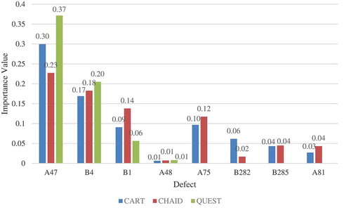
2The most important defects identified by the CART and CHAID algorithms were “Failure to log the construction journal” (A75), “Other recording errors in building material and equipment reviews” (B282), “Failure to install required fall protection facilities” (B285), and “Lack of quality control statistical analysis” (A81). The predictive abilities for these four defects were nonsignificant in the QUEST algorithm. Therefore, the corresponding nonsignificant input attributes were deleted.

5.1. CART algorithm

The DT constructed using the CART algorithm is presented in Figure 2, indicating four attribute. The target attribute in the root node represents the project grades. The improvement measures for the three attribute levels are described as follows:

Figure 2. Structural model of the CART algorithm.

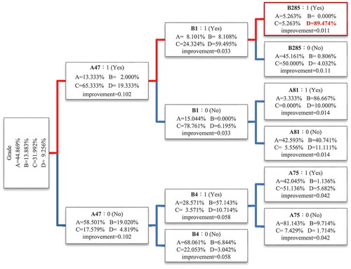
1. The first-layer attribute was “A47,” with the improvement measure being 0.102.

2. The second-layer attributes were “B1” and “B4,” with the improvement measures being 0.033 and 0.058, respectively.

3. The third-layer attributes were “B285,” “A81,” and “A75,” with the improvement measures being 0.011, 0.014, and 0.042, respectively.

5.2. CHAID and QUEST algorithms

The DT structures constructed using the CHAID and QUEST algorithms are shown in Figures 3 and 4, respectively. The structural model constructed using the CHAID algorithm exhibited five layers of attributes, and the tree structure was more complicated than those of the models constructed using the CART and QUEST algorithms. The tree structure of the model constructed using the QUEST algorithm was the simplest. The p value and chi-squared value of the three different attribute layers are described as follows:

Figure 3. Structural model constructed using the CHAID algorithm.

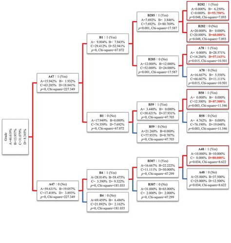
Figure 4. Structural model constructed using the QUEST algorithm.

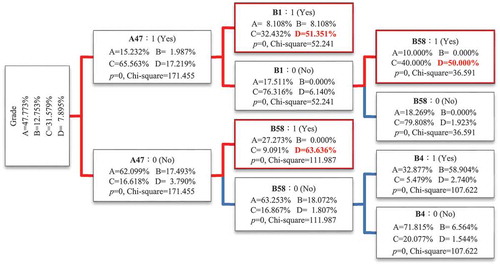
The first-layer attribute was “A47,” with the p value being 0 and chi-squared value being 171.455. Two second-layer attributes were observed: “B1,” with the p value being 0 and chi-squared value being 52.241,” and “B58,” with the p value being 0 and chi-squared value being 111.987. Furthermore, two third-layer attributes were observed: “B58,” with the p value being 0 and chi-squared value being 36.591, and “B4,” with the p value being 0 and chi-squared value being 107.622.

5.3. Defect detection rules derived using three algorithms

DT analysis focuses on specific attributes of a target by examining its past behaviors to conduct estimations. For example, if long-term monitoring reveals that people who are long-term smokers, work in environments with severe air pollution, and frequently consume high-fat foods have an 80% chance of developing lung cancer on average, then one of the three aforementioned factors must be eliminated to reduce the risk of developing lung cancer. In the case of a construction project, if defects I, II, and III lead to unfavorable project quality and result in an 80% chance of receiving Grade D, then these defects should be avoided to improve the project grade.

This study employed the CART, CHAID, and QUEST algorithms to generate DTs and calculated the possibility of project grades according to nine defect rules (Table 4). Each rule was mainly focused on the defects of D for determining the conditions that may result in poor grades. The relationship between the defects could be determined using these nine rules and the percentages of the four grades of the DTs (A, B, C, and D).

Table 4. Defect rules for CART, CHAID, and QUEST.

Algorithm	Rules	Project grades (%)
		A	B	C	D
CART 1	if A47 = 1 & B285 = 1 & B1 = 1 then D	5.26	0	5.26	89.48
CHAID 1	if A47 = 1 & B1 = 1 & B285 = 1 & B282 = 1 then D	0	6.25	0	93.75
CHAID 2	if A47 = 1 & B1 = 1 & B285 = 1 & B282 = 0 then D	20.00	0	20.00	60.00
CHAID 3	if A47 = 1 & B1 = 1 & B285 = 0 & A78 = 1 then D	0	28.57	14.29	57.14
CHAID 4	if A47 = 1 & B1 = 0 & B59 = 1 & B58 = 1 then D	0	0	12.50	87.50
CHAID 5	if A47 = 0 & B4 = 1 & B307 = 1 & A48 = 1 then D	10.00	10.00	0	80.00
QUEST 1	if A47 = 1 & B1 = 1 then D	8.11	8.11	32.43	51.35
QUEST 2	if A47 = 1 & B1 = 0 & B58 = 1 then D	10.00	0	40.00	50.00
QUEST 3	if A47 = 0 & B58 = 1 then D	27.27	0	9.09	63.64

Consider, for example, the rule CART 1. If the defects included in this rule were “Failure to inspect construction works and equipment” (A47), “Failure to install required fall protection facilities” (B285), and “Substandard concrete pouring or ramming” (B1), the probability of predicting a grade D defect was 89.48%, whereas that for predicting both grade A and C was 5.26%. The rule CHAID 5. If the defects included in this rule were “Inspect construction works and equipment” (A47), “Debris on concrete surface” (B4), “Failure to install facilities to protect against injury or stabbing induced by sharp objects in the workplace” (B307), and “No supervisory contractor performs site-safety-related and health-related tasks” (A48), the probability of predicting a grade D defect was 80%, whereas that for predicting both grade A and B was 10%. Accordingly, to improve project quality and avoid receiving a poor inspection grade (Grade D), the occurrence of defects specified in the aforementioned rules should be reduced. Furthermore, these rules can be used as critical evaluation items when monitoring a construction project.

Among them, CHAID 1 had the highest probability of predicting grade D defects, which could be as high as 93.75%. The difference between CHAID 1 and CART 1 (89.48%) can be explained by the fact that CHAID 1 included “Other recording errors in building material and equipment reviews” (B282).

The CART algorithm had only one rule (89.45%) for the grade D, and the CHAID algorithm had five classification rules. The probabilities of these five rules predicting grade D were between 57.14% and 93.75%. The QUEST algorithm had the lowest probabilities of predicting grade D, which were between 50% and 63.63%. This reveals that the QUEST algorithm had a relatively poor predictive ability in terms of the classification of data in the PCMIS database.

In this study, defect data were classified by being categorized into multiple tree-shaped hierarchical levels. Each level contained one or multiple nodes (defects), and each node contained the percentage value of four project grades (namely grades A, B, C, and D). The optimal scenario is the percentage value of grade D being 100% in each node. However, achieving this scenario is highly unlikely, meaning that regardless of the input variables used to generate a child node, the data distribution would contain impurities. Generally, the node that generates the highest data purity is adopted to interpret and establish rules. The DT algorithms used in this study are valuable because they can be used to analyze inspection records to identify defects (nodes) that most accurately predict the occurrence of grade D, thereby determining the applicability and logic of using these defects to evaluate construction management.

5.4. Analysis of effect of the algorithms

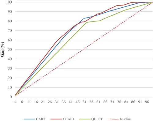
Several DT algorithms have been developed and each of such algorithms has inherent inferential characteristics. In addition, each of such algorithms is suitable for distinct databases and has some advantages and disadvantages. A gain chart is used to compare model classification results; moreover, a confusion matrix is used to determine prediction accuracy.

A gain chart is the most commonly used method for evaluating DM models, and the horizontal and vertical axes represent percentages. The percentages on the horizontal axis are sorted on the basis of probability from high to low and represent the percentages of the test data set. The vertical axis represents the percentages of the actually predicted values. An upward curve of a gain chart indicates that the more effective the model is, the greater is the area under the curve (AUC). If the model’s cumulative gain curve displays a 45° angle with the horizontal axis, then the model is a random model, and the predicted effect cannot be classified.

The lowest defect prediction accuracy in this study was observed for the QUEST algorithm. The CART and CHAID algorithms exhibited similar classification results. The first 40% of the CART and CHAID test data sets can predict actual values of 70.41% and 69.13%, respectively; QUEST is only 60.16% (Figure 5).

Figure 5. Gain chart for CART, CHAID, and QUEST.

A confusion matrix is used to compare model predictions with test data to determine the effectiveness of a classification model. Thus, it can be used to evaluate the performance of supervised classification processes.

For an ideal model, the predicted values must match the actual values. However, most model predictions are not 100% accurate. For example, a set of attributes that belonged to the A category were predicted by a DT algorithm to belong to the B category. Therefore, a confusion matrix was required to analyze the recall and accuracy of model predictions. The confusion matrix was used to present all the classification information in a complete matrix.

Table 5 presents the recall and accuracy of the three algorithms. The recall for a category is the number of predictions in the category divided by the actual number of members of the category. For example, the CART algorithm correctly predicted 380 entries as belonging to grade A; therefore, the corresponding recall was 82.97%, as obtained by dividing the number of correctly predicted entries by the total number of entries in A (458). Among the three algorithms, the CART algorithm had the lowest prediction for grade D (37.23%); the CHAID algorithm had a relatively average prediction for all four grades-A, B, C, and D.

Table 5. Confusion matrix and accuracy for DT generation.

Algorithm	n=990	Predicated				Total	Recall (%)	Classification accurate (%)
	Actual	A	B	C	D
CART	A	380	14	62	2	458	82.97	73.33
	B	46	84	4	1	135	62.22
	C	68	4	227	4	303	74.92
	D	8	19	32	35	94	37.23
CHAID	A	351	39	65	3	458	76.64	75.45
	B	35	93	3	4	135	68.89
	C	53	4	239	7	303	78.88
	D	10	4	16	64	94	68.09
QUEST	A	359	43	38	18	458	78.38	68.38
	B	34	97	0	4	135	71.85
	C	117	4	150	32	303	49.50
	D	6	10	7	71	94	75.53

Accuracy can be defined as the number of correct predictions across all categories divided by the total number of entries. For example, the CART algorithm correctly predicted 380, 84, 227, and 35 entries for grades A, B, C, and D, respectively. The summation of these values divided by the total number of entries in all grades (990) yielded an accuracy of 73.33%. The accuracy rates of the CART, CHAID, and QUEST algorithms were 73.33%, 75.45%, and 68.38%, respectively. Accordingly, the CHAID algorithm had the highest prediction accuracy.

The three DT models constructed in this study exhibited an accuracy between 68% and 76%. Table 5 lists the number of predictions and corresponding percentages of each project grade. The accuracy was calculated based on factors such as the number of samples in the database, number of samples used for model training and testing, types of target variables and attributes, and data complexity. Compared with models constructed by similar studies in the field of construction that were conducted recently, those used in this study exhibited favorable accuracy; for example, the CHAID and C5.0 algorithms used by Mistikoglu et al. (2015) attained accuracies of 66.8% and 67.9%, respectively. The present study verified the feasibility of the three models. In particular, the CHAID algorithm performed most favorably in terms of classification and prediction.

DT works in the way of using information gain derived from information theory to find the position for the maximum amount of information in the data set so as to establish the nodes of the DT, in which each node will encounter a test, and the test results (from different problems on the node) will lead to different branches. Ultimately, the classification process will decide on the category according to a number of variables, and a leaf node will be reached, which is the category result of the classification. It can be used to explore the relationships between a large number of candidate input attributes and an output (target) attribute. This method systematically entails breaking down and subdividing the information contained in a dataset, thus creating a top-down branching structure.

In order to further understand the relationship between various attribute variables and qualities (project grades) of the project, the DT Model was drawn up as follows: the input decision variables were 499 defect types (Code: Ai, Bi, Ci, Di) and three project attributes (contract sums, project category, and progress); the output target variable was project grades. As a result, six decision tree rules were generated (see Table 6), and the results showed that the three project attributes (contract sums, project category, and progress) as mentioned earlier did not appear on the branch nodes, which suggests that the impact of these three attributes on the project grade was minor. The impact of the quality of the project was still decided by the quantities of defects. Thus, the committee members’ inspection scores on the project quality had no certain correlation with the type or size of the project.

Table 6. Project attributes rules for CART, CHAID, and QUEST.

Algorithm	Rules	Project grades (%)
		A	B	C	D
CART 1	if B4 = 1 & A47 = 0 & A29 = 0 & B307 = 1 then D	22.22	11.11	11.11	55.56
CART 2	if A47 = 1 & B285 = 1 & B1 = 1 then D	12.50	6.25	12.50	68.75
CHAID 1	if A47 = 1 & B14 = 0 & A38 = 0 & B58 = 1 & A68 = 1 then D	20.00	0	0	80.00
CHAID 2	if A47 = 1 & B14 = 0 & A38 = 1 & B285 = 1 then D	0	0	18.18	81.82
CHAID 3	if A47 = 1 & B14 = 1 then D	6.67	13.33	6.67	73.33
QUEST 1	if B1 = 1 & B258 = 1 then D	17.24	13.79	6.90	62.07

Additionally, through the evaluation four attributes from the confusion matrix, the accuracy rates of CART, CHAID and, QUEST, the three DT algorithms, were 72.83%, 71.82%, and 65.45%, respectively. Statistically speaking, as the DT input variables increase and because correlation and multiplicity exist between the attributes, the data set division will be dwindled, resulting in poor prediction accuracy. Also, the classification effectiveness (gain chart) has indicated that the first 40% of the CART, CHAID, and QUEST test data sets could predict their actual values of 64.25%, 68.11%, and 60.81%, respectively. It is seen that there was a large decrease in the actual values of CART by 6.16%, and the actual decreased values (0.65%-1.02%) in CHAID and QUEST were not significant.

6. Conclusion

DT algorithms were used in this study to compare the efficiency and accuracy of the CART, CHAID, and QUEST. Classification rules were developed for defects by using data from the PCMIS construction inspection database. This helps construction managers to quickly classify and predict the quality grades of their projects and identify factors contributing to unfavorable construction quality. The algorithm providing the most accurate classifications was identified. The results can serve as a reference for project management units in applying optimal classification algorithms and developing appropriate defect management strategies.

The results of this study revealed that “Failure to inspect construction works and equipment” (A47) was the most important defect. The following is the sequence of defects in the order of importance: “Debris on concrete surface” (B4), “Substandard concrete pouring or ramming” (B1), and “No supervisory contractor performs site-safety-related and health-related tasks” (A48). The four aforementioned defects affect the project grade and are crucial for project management.

The CHAID algorithm determines the results of individual defects and successfully classifies data to effectively determine importance values of defects. The CHAID algorithm generates five rules of different complexity degrees that are links between grades and defects. The CHAID algorithm generates more rules than the CART and QUEST algorithms do, and this can be considered an informational advantage for the CHAID algorithm. The prediction accuracy observed for the CHAID algorithm was 75.45% in this study, thus demonstrating that defects could be accurately predicted and signifying that the rules can be applied to perform defect management.

Construction projects have varying degrees of complexity. When 499 defect types are found during a construction inspection, all resources cannot be used for ensuring efficient defect management. Therefore, project managers must select the most crucial defects for implementation in control mechanisms. In particular, the defects directly affect project grades. To establish an ideal project management system, appropriate analytical tools and methods must be selected to directly explain the rules and importance values of defects. Training and testing defect data can be used to determine the optimal DT algorithm for defect identification, which can facilitate site management tasks. The analysis results of this study can serve as a reference for construction teams to effectively improve the quality and performance of projects.

This study was limited in that a binary approach was used to code defect data. Such an approach only determines whether an attribute exists in each rule. In practice, attributes that do not exist in a rule are difficult to explain. Each DT model has unique characteristics. When applying a DT model to a classification or prediction problem concerning a real-world scenario, the selection of parameters, attribute types (continuous or discrete), and training and testing subsets should align with the characteristics of the problem in question. This enables the identification of an adequate combination of input variables to construct a DT with optimal classification and prediction accuracy. Furthermore, the multi-attribute variable test results in this study have shown that to improve the accuracy of the classification, the attributes that are not related to the classification target must be deleted before the selection of the DT classifier.

Correction Statement

This article has been republished with minor changes. These changes do not impact the academic content of the article.

Disclosure statement

No potential conflict of interest was reported by the authors.

References

- Ahzahar, N., N.A. Karim, S.H. Hassan, and J. Eman. 2011. “A Study of Contribution Factors to Building Failures and Defects in Construction Industry.” Procedia Engineering 20: 249–255. doi:10.1016/j.proeng.2011.11.162.
- Alipour, M., D. K. Harris, L. E. Barnes, and O. E. Ozbulut. 2017. “Load-capacity Rating of Bridge Populations through Machine Learning: Application of Decision Trees and Random Forests.” Journal of Bridge Engineering 22: 10. doi:10.1061/(ASCE)BE.1943-5592.0001103.
- Aljassmi, H., and S. Han. 2013. “Analysis of Causes of Construction Defects Using Fault Trees and Risk Importance Measures.” Journal of Construction Engineering and Management 139 (7): 870–880. doi:10.1061/(ASCE)CO.1943-7862.0000653.
- Aljassmi, H., S. Han, and S. Davis. 2016. “Analysis of the Complex Mechanisms of Defect Generation in Construction Projects.” Journal of Construction Engineering and Management 142: 2. doi:10.1061/(ASCE)CO.1943-7862.0001042.
- Arditi, D., and T. Pulket. 2005. “Predicting the Outcome of Construction Litigation Using Boosted Decision Trees.” Journal of Computing in Civil Engineering 19 (4): 387–393. doi:10.1061/(ASCE)0887-3801(2005)19:4(387).
- Atkinson, A. R. 1999. “The Role of Human Error in Construction Defects.” Structural Survey 17 (4): 231–236. doi:10.1108/02630809910303006.
- Breiman, L., J. H. Friedman, R. J. Olshen, and C. J. Stone. 1984. Classification and Regression Trees. Belmont, California: Wadsworth International Group.
- Brijs, T., K. Vanhoof, and G. Wets. 2003. “Defining Interestingness for Association Rules.” International Journal of Information Theories and Applications 10 (4): 370–375.
- Cain, C. T. 2004. Performance Measurement for Construction Profitability. Oxford: Blackwell.
- Chan, A. P. C., D. Scott, and E. W. M. Lam. 2002. “Framework of Success Criteria for Design/build Projects.” Journal of Management in Engineering 18 (3): 120–128. doi:10.1061/(ASCE)0742-597X(2002)18:3(120).
- Chen, Y. L., C. L. Hsu, and S. C. Chou. 2003. “Constructing a Multi-valued and Multilabeled Decision Tree.” Expert Systems with Applications 25 (2): 199–209. doi:10.1016/S0957-4174(03)00047-2.
- Cheng, Y., W. D. Yu, and Q. Li. 2015. “GA‐based Multi-level Association Rule Mining Approach for Defect Analysis in the Construction Industry.” Automation in Construction 51: 78–91. doi:10.1016/j.autcon.2014.12.016.
- Cheng, Y. M., and S. S. Leu. 2011. “Integrating Data Mining with KJ Method to Classify Bridge Construction Defects.” Expert Systems with Applications 38: 7143–7150. doi:10.1016/j.eswa.2010.12.047.
- Chien, C., W. Wang, and J. Cheng. 2007. “Data Mining for Yield Enhancement in Semiconductor Manufacturing and an Empirical Study.” Expert Systems with Applications 33 (1): 192–198. doi:10.1016/j.eswa.2006.04.014.
- Chong, W. K., and S. P. Low. 2005. “Assessment of Defects at Construction and Occupancy Stages.” Journal of Performance of Constructed Facilities 19 (4): 283–289. doi:10.1061/(ASCE)0887-3828(2005)19:4(283).
- Chou, J. S., S. C. Hsu, C. W. Lin, and Y. C. Chang. 2016. “Classifying Influential Information to Discover Rule Sets for Project Disputes and Possible Resolutions.” International Journal of Project Management 34 (8): 1706–1716. doi:10.1016/j.ijproman.2016.10.001.
- Chou, P. A. 1991. “Optimal Partitioning for Classification and Regression Trees.” IEEE Transactions on Pattern Analysis and Machine Intelligence 13: 340–354. doi:10.1109/34.88569.
- Chua, D. K. H., Y. C. Kog, and P. K. Loh. 1999. “Critical Success Factors for Different Project Objectives.” Journal of Construction Engineering and Management 125 (3): 142–150. doi:10.1061/(ASCE)0733-9364(1999)125:3(142).
- Das, S., and M. Y. L. Chew. 2011. “Generic Method of Grading Building Defects Using FMECA to Improve Maintainability Decisions.” Journal of Performance of Constructed Facilities 25 (6): 522–533. doi:10.1061/(ASCE)CF.1943-5509.0000206.
- Efraim, T., S. Ramesh, and D. Dursun. 2010. Decision Support and Business Intelligence Systems. 9th ed. Upper Saddle River, NJ: Prentice Hall.
- Forcada, N., M. Macarulla, M. Gangolells, M. Casals, A. Fuertes, and X. Roca. 2013. “Post-handover Housing Defects: Sources and Origins.” Journal of Performance of Constructed Facilities 27 (6): 756–762. doi:10.1061/(ASCE)CF.1943-5509.0000368.
- Han, J., and M. Kamber. 2001. Data Mining Concept and Technology. San Francisco: Morgan Kaufmann.
- Han, S. H., S. X. Lu, and S. C. H. Leung. 2012. “Segmentation of Telecom Customers Based on Customer Value by Decision Tree Model.” Expert Systems with Applications 39 (4): 3964–3973. doi:10.1016/j.eswa.2011.09.034.
- Josephson, P. E., and Y. Hammarlund. 1999. “The Causes and Costs of Defects in Construction: A Study of Seven Building Projects.” Automation in Construction 8 (6): 681–687. doi:10.1016/S0926-5805(98)00114-9.
- Kass, G. V. 1980. “An Exploratory Technique for Investigating Large Quantities of Categorical Data.” Applied Statistics 29 (2): 119–127. doi:10.2307/2986296.
- Khan, F. S., R. M. Anwer, O. Torgersson, and G. Falkman. 2009. “Data Mining in Oral Medicine Using Decision Trees.” International Journal of Biological and Medical Sciences 4: 156–161.
- Kim, Y. S. 2008. “Comparison of the Decision Tree, Artificial Neural Network, and Linear Regression Methods Based on the Number and Types of Independent Variables and Sample Size.” Expert Systems with Applications 34 (2): 1227–1234. doi:10.1016/j.eswa.2006.12.017.
- Kumar, P. R., and V. Ravi. 2007. “Bankruptcy Prediction in Banks and Firms via Statistical and Intelligent Techniques-a Review.” European Journal of Operational Research 180: 1–28. doi:10.1016/j.ejor.2006.08.043.
- Lee, M. J., A. S. Hanna, and W. Y. Loh. 2004. “Decision Tree Approach to Classify and Quantify Cumulative Impact of Change Orders on Productivity.” Journal of Computing in Civil Engineering 18 (2): 132–144. doi:10.1061/(ASCE)0887-3801(2004)18:2(132).
- Lee, S., S. Han, and C. Hyun. 2016. “Analysis of Causality between Defect Causes Using Association Rule Mining. International Journal of Civil.” Environmental, Structural, Construction and Architectural Engineering 10 (5): 654–657.
- Lin, C. L., and C. L. Fan. 2018. “Examining Association between Construction Inspection Grades and Critical Defects Using Data Mining and Fuzzy Logic.” Journal of Civil Engineering and Management 24 (4): 301–315. doi:10.3846/jcem.2018.3072.
- Lin, W. T., S. T. Wang, T. C. Chiang, Y. X. Shi, W. Y. Chen, and H. M. Chen. 2010. “Abnormal Diagnosis of Emergency Department Triage Explored with Data Mining Technology: An emergency department at a Medical Center in Taiwan Taken as an Example.” Expert Systems with Applications 37 (4): 2733–2741. doi:10.1016/j.eswa.2009.08.006.
- Loh, W., and Y. Shih. 1997. “Split Selection Methods for Classification Trees.” Statistica Sinica 7: 815–840.
- Macarulla, M., N. Forcada, M. Casals, M. Gangolells, A. Fuertes, and X. Roca. 2013. “Standardizing Housing Defects: Classification, Validation, and Benefits.” Journal of Construction Engineering and Management 139 (8): 968–976. doi:10.1061/(ASCE)CO.1943-7862.0000669.
- Meng, X. 2012. “The Effect of Relationship Management on Project Performance in Construction.” International Journal of Project Management 30: 188–198. doi:10.1016/j.ijproman.2011.04.002.
- Mistikoglu, G., I. H. Gerek, E. Erdis, P. E. M. Usmen, H. Cakan, and E. E. Kazan. 2015. “Decision Tree Analysis of Construction Fall Accidents Involving Roofers.” Expert Systems with Applications 42 (4): 2256–2263. doi:10.1016/j.eswa.2014.10.009.
- Munns, A. K., and B. F. Bjeirmi. 1996. “The Role of Project Management in Achieving project Success.” International Journal of Project Management 14 (2): 81–87. doi:10.1016/0263-7863(95)00057-7.
- Neville, P.G. 1999. “Decision Trees for Predictive Modeling.” Cary, NC:Sas Institute Inc.
- Piramuthu, S. 2008. “Input Data for Decision Trees.” Expert Systems with Applications 34: 1220–1226. doi:10.1016/j.eswa.2006.12.030.
- Robert, T.R. 2005. Structural Condition Assessment. Hoboken, NJ: John Wiley & Sons, Inc.
- Rodrigues, J., D. Folgado, D. Belo, and H. Gamboa. 2019. “SSTS: A Syntactic Tool for Pattern Search on Time Series.” Information Processing & Management 56: 61–76. doi:10.1016/j.ipm.2018.09.001.
- Ryua, Y. U., R. Chandrasekaranb, and V. S. Jacobc. 2007. “Breast Cancer Prediction Using the Isotonic Separation Technique.” European Journal of Operational Research 181 (2): 842–854. doi:10.1016/j.ejor.2006.06.031.
- Shenhar, A. J., D. Dvir, O. Levy, and A. C. Maltz. 2001. “Project Success: A Multidimensional Strategic Concept.” Journal of Long Range Planning 34 (6): 699–725. doi:10.1016/S0024-6301(01)00097-8.
- Shin, Y., T. Kim, H. Cho, and K. I. Kang. 2012. “A Formwork Method Selection Model Based on Boosted Decision Trees in Tall Building Construction.” Automation in Construction 23: 47–54. doi:10.1016/j.autcon.2011.12.007.
- Shirazi, F., and M. Mohammadi. 2019. “A Big Data Analytics Model for Customer Churn Prediction in The Retiree Segment.” International Journal Of Information Management 48: 238-253. doi:10.1016/j.ijinfomgt.2018.10.005.
- Shirkavand, I., J. Lohne, and O. Lædre. 2016. “Defects at Handover in Norwegian Construction Projects.” Procedia Social and Behavioral Sciences 226: 3–11. doi:10.1016/j.sbspro.2016.06.155.
- Sommerville, J. 2007. “Defects and Rework in New Build: An Analysis of the Phenomenon and Drivers.” Structural Survey 25 (5): 391–407. doi:10.1108/02630800710838437.
- Syachrani, S., H. S. Jeong, and C. S. Chung. 2013. “Decision Tree-based Deterioration Model for Buried Wastewater Pipelines.” Journal of Performance of Constructed Facilities 27 (5): 633–645. doi:10.1061/(ASCE)CF.1943-5509.0000349.
- Tayefia, M., M. Tajfard, S. Saffar, P. Hanachi, A. R. Amirabadizadeh, H. Esmaeily, A. Taghipour, G. A. Ferns, M. Moohebati, and M. Ghayour-Mobarhan. 2017. “hs-CRP Is Strongly Associated with Coronary Heart Disease (CHD): A Data Mining Approach Using Decision Tree Algorithm.” Computer Methods and Programs in Biomedicine 141: 105–109. doi:10.1016/j.cmpb.2017.02.001.
- Ture, M., F. Tokatli, and I. Kurt. 2009. “Using Kaplan-Meier Analysis Together with Decision Tree Methods (C&RT, CHAID, QUEST, C4.5 And ID3) in Determining Recurrence-free Survival of Breast Cancer Patients.” Expert Systems with Applications 36 (2): 2017–2026. doi:10.1016/j.eswa.2007.12.002.
- Varlamis, I., I. Apostolakis, D. Sifaki-Pistolla, N. Dey, V. Georgoulias, and C. Lionis. 2017. “Application of Data Mining Techniques and data Analysis Methods to Measure Cancer Morbidity and Mortality data in a Regional cancer Registry: The Case of the Island of Crete, Greece.” Computer Methods and Programs in Biomedicine 145: 73–83. doi:10.1016/j.cmpb.2017.04.011.
- Xiao, F., and C. Fan. 2014. “Data Mining in Building Automation System for Improving building Operational Performance.” Energy and Buildings 75: 109–118. doi:10.1016/j.enbuild.2014.02.005.
- Yeoa, B., and D. Grant. 2018. “Predicting Service Industry Performance Using Decision Tree Analysis.” International Journal of Information Management 38 (1): 288–300. doi:10.1016/j.ijinfomgt.2017.10.002.