Minimum number of simulation runs for reliable building energy and peak load prediction at different building scales: a study on stochastic shade adjustment

ABSTRACT

This paper investigates the impact of uncertain shade behavior on three facades (east, south and west) on energy performance. A previously developed stochastic shade behavior model and an occupancy model were used to conduct building co-simulation for determining energy-related performance uncertainty (annual energy demand and peak heating/cooling loads) at different building scales. Statistical test and Monte Carlo random sampling techniques were used to determine the required minimum simulation runs for obtaining reliable annual energy performance and peak loads. The results show that there is no significant difference in shading performance among seasons and orientations. In China, most newly-built office buildings are high-rise ones and thus, the influence of manual shades on the energy uncertainty of these office buildings can be neglected and a single simulation run is enough to obtain reliable annual heating, cooling and total energy demands. While for peak heating/cooling loads, the conclusion is different from annual energy demand and at least five simulation runs are required to obtain peak heating/cooling loads at building scales. For a smaller building, 120 simulation runs are suggested for peak load determination.

KEYWORDS:

• Manual shades
• uncertainty
• building energy
• peak load
• number of simulation runs

1. Introduction

Occupant behavior has been recognized as a major source of gaps between predicted and actual energy performance (Yan et al. 2017; Gilani, O’Brien, and Gunay 2018; Haldi and Robinson 2011; Delzendeh et al. 2017). For example, the energy prediction obtained from simulation tools typically deviates by more than 30% from actual energy consumption levels (Soebarto and Williamson 2001; Azar and Menassa 2012). Occupant behavior also leads to a significant building energy uncertainty. A study by Clevenger and Haymaker (Clevenger and Haymaker 2006) found that energy consumption might change by more than 150% if occupants have different energy patterns. Andersen, Olesen, and Jørn (Andersen, Olesen and Toftum 2007) found that building energy performance could vary by 324% from a low consumption scenario to a high consumption one. Therefore, it is important to consider realistic occupant behavior in building performance simulation for a higher prediction accuracy.

To understand occupant behavior patterns, field monitoring and survey studies of occupant behavior and related environmental factors have been conducted. For example, occupancy (Page et al. 2008; Li and Dong 2017), window opening (Yao and Zhao 2017; Andersen et al. 2013; Lai et al. 2018), light switching (Gilani and O’Brien 2018; Reinhart 2004; Zhu et al. 2017), air-conditioning (Yao 2018b; Ren, Yan, and Wang 2014), shade/blind adjustment (Reinhart and Voss 2003; Haldi and Robinson 2010) have been investigated and different types of occupant behavior models have been developed for integration into building performance simulation tools. Modern office buildings are mostly designed with large windows for a better daylighting performance, and some of them have glazed curtain walls. The negative impact of large windows includes glare risks, overheating and higher cooling energy demands. Thus, almost all of these buildings in China are installed with internal top-down roller shades operated manually due to its low cost and maintenance.

To date, a few shade behavior models have been reported. For example, Newsham’s study (Newsham 1994) proposed a shade model that was based on solar radiation. In this model, shades were closed when solar intensity on indoor occupants was higher than 233 W/m². Reinhart’s shade model (Reinhart 2004) assumed that manual shades were closed when direct solar irradiance on workplane is over 50 W/m². Similar shade models or assumptions based on workplane illuminance, solar radiation, luminance and glare indexes have been reported in review studies (Da Silva, Leal, and Andersen 2012; Yun, Park, and Kim 2017; O’Brien, Kapsis, and Athienitis 2013). However, these shade models or assumptions did not consider partial shading states (only fully open and fully closed scenarios were considered), which is not in line with realistic shade adjustment that most shade positions are deployed at intermediate positions (Correia Da Silva, Leal, and Andersen 2013; Yao 2014). In addition, some of these models are deterministic rather than stochastic, leading to a deterministic energy performance. This is also not in line with the fact that realistic energy performance is uncertain.

To overcome the limitations of the fully open and closed shade models, Haldi and Robinson (2010) developed an improved shade behavior model based on logistic regression curves with partial shading states being considered. This model is based on a rather unusual motorized shading system, which is different from manual solar shades widely used in China. Thus, the shade behavior pattern (67.1% of occupied time is fully opened) is different from that in Chinese office buildings (Yao 2014). Therefore, this model is not applicable to office buildings in China. In addition, this model is not applicable to east and west facades since it was developed based on south-facing windows.

To investigate the influence of manual shades on energy performance in China, a shade behavior model for east, south and west facades was developed based on a typical office building with internal top-down roller shades. This model has the benefits of considering partial shading states and was validated with realistic shade behavior patterns in that building. Energy, thermal, visual and life cycle economic performance of manual shades have been studied (Yao 2014; Yao et al. 2016; Yao 2018a; Yao, Chow, and Chi 2016; Yao 2019; Yao and Zheng 2019). This paper is a continuation of previous research and the focus of the current research is: (1) to compare shading performance difference between east, south and west facades; (2) to compare the difference in energy performance and uncertainty levels among the three facades; and (3) to determine the minimum number of simulation runs to obtain reliable annual energy and peak heating/cooling loads at different building scales. According to recent literature reviews on manual shades (Delzendeh et al. 2017; O’Brien, Kapsis, and Athienitis 2013; Hong et al. 2018; Gunay, O’Brien, and Beausoleil-Morrison 2013), these three aspects have not been studied, especially in Chinese office buildings. Therefore, the findings of this research may benefit practitioners in manual shade-related building performance analysis.

2. Methodology

2.1. Shade behavior model and simulation setting

2.1.1. Room model

To investigate the impact of manual shades on energy performance, a typical office cell was considered in this paper with dimensions of 4 × 4 × 3 m (width×length×height). The model has an external wall with a 3.8 × 2.8 m (width×height) window as shown in Figure 1 (the other three walls were treated as internal walls). Three orientations (east, south and west) were considered by rotating the building model. The simulation setting of the office cell (including the setting of manually controlled shading devices) is shown in Table 1.

Figure 1. Office cell model.

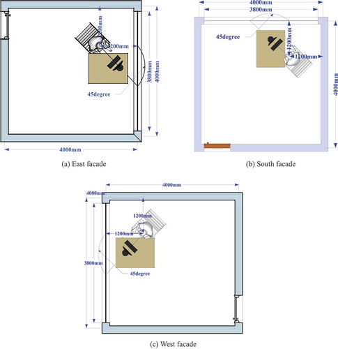
Table 1. Simulation setting.

Parameter	Value
Location	Hangzhou city in China, latitude: 30°, longitude: 120°
Orientation	East, south, west
Dimension	Office cell: 4 × 4 × 3 m, Window: 3.8 × 2.8 m
Window and shading device	Clear double-pane window: U-value: 3.6 W/m^2 K and Tv: 0.78, SHGC of the glazing: 0.698; Manually controlled internal roller shades, shade material: visual transmittance: 0.2. Shade behavior model: described in section 2.1.2
Opaque envelope	U-value for external wall:1 W/m^2 K; Internal walls, roof and floor: adiabatic
Office hours	Occupancy model: described in section 2.1.1
HVAC	Temperature set-points for heating and cooling: 20°C and 26°C, Temperature setback for heating and cooling: 5°C and 37°C Operation time: on during occupancy
Interior heat generation	Light power density (LPD): 11 W/m^2; equipment: 20 W/m^2
Breathing zone outdoor airflow	40 m^3/h.p

2.1.2. Occupancy model

To consider occupancy state, Page et al.’s (2008) occupancy algorithm was adopted. This model inputs the profile of probability of presence and the parameter of mobility and generates a time series (here it is whole year) of the state of presence (absent or present) based on Markov chain method. More detailed information of this algorithm can be found in (Page et al. 2008). To use this model, observation of occupancy state in seven office rooms was conducted using passive infrared (PIR) motion sensors.

2.1.3. Shade behavior model

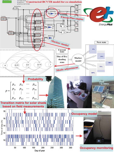
The shade behavior model used in this paper was developed based on field measurements on a highly glazed tall building in hot summer and cold winter zone of China. This model considered five discrete shade positions (fully open, 75% open, 50% open, 25% open and fully closed) and thus five shading coefficients (SC = 1, 0.75, 0.5, 0.25 and 0) were used to represent these five shading states. For example, SC = 0.75 represents 75% open. The developed shade behavior model was based on the discrete-time Markov chain method and the stochastic adjustment of manual shades in next time step was predicted based on the shade position in the current step and current solar intensity on the façade (east, south and west façades were considered, respectively). The shade behavior model was modeled in Building Controls Virtual Test Bed (BCVTB) for co-simulation with EnergyPlus–an energy simulation engine developed by Lawrence Berkeley National Laboratory. More detailed information on this stochastic model and the co-simulation can be found in the previous paper (Yao 2014). A graphic illustration of the stochastic shade model combined with the occupancy model is shown in Figure 2.

Figure 2. A graphic illustration of the developed method for co-simulation of energy performance of manual solar shades based on occupancy and shade behavior models.

2.2. Distribution of energy performance

Since the developed shade behavior model represents occupants’ random interaction with solar shades, the simulation output of this behavior model is stochastic. Thus, repeated simulation runs are needed to obtain the possible distribution of the simulation output (cooling, heating and total energy demands). To have a balance between computational cost and high accuracy, a suitable number of simulation runs was determined according to the graphical method recommended in (Robinson 2014), which has been used for similar analysis in previous papers (Yao and Zheng 2019; Chapman, Siebers, and Robinson 2018). The minimum number of repeated simulations required is defined by the point at which the line (the cumulative mean of the simulated annual energy demand) becomes flat. In this paper, 100 simulation runs were conducted and the mean value of the fitted distribution was considered as the true mean energy demand since previous research has confirmed that this number was enough for determining the distribution of energy data (Gilani, O’Brien, and Gunay 2018; Yao 2019; Macdonald 2009).

2.3. Number of simulation runs for annual energy performance

For uncertainty of annual energy performance, the probability distribution function was used to fit to the annual energy data. In this paper, normal distribution was adopted (since the following analysis in section 3.2 confirmed the normal distribution of the data) and can be expressed as a function f(x), where x is the annual energy demand (cooling, heating and total). In common cases, f(x) could be determined by the mean and the variance of f(x), which can be modeled as a hypothesis problem (see below).

The Hypothesis: the estimated mean value E is equal to the mean in the distribution and expressed as H0: E = μ.

The selected parametric test is Ф: H0 is accepted when |E-μ|≤C, and rejected otherwise.

where E is the mean of the simulated energy demand. In statistics, a confidence level of 1-α can be expressed as

(1) $1-\alpha \le P_{\mu }(|E-\mu |\le C)$(1)

For a hypothesis testing problem, the sample size n is already known (here it is 100), and Equation 1(1) $1-\alpha \le P_{\mu }(|E-\mu |\le C)$(1) is used to determine a suitable C which is based on the selected confidence level. The probability distribution of E (denoted by E ~ φ(x,n)) can be determined since the distribution of x is already known and Equation 1(1) $1-\alpha \le P_{\mu }(|E-\mu |\le C)$(1) can be converted to:

(2) $1-\alpha \le P_{\mu }(\mu -C\le \varphi (x,n)\le \mu +C)$(2)

The probability distribution function of E can be expressed as

(3) $E\text{~}N\left(\mu ,\frac{{\sigma }^2}{n}\right)$(3)

The derived statistic T is

(4) $T=\frac{\sqrt{n}(E-\mu )}{\sigma }$(4)

Equation 2(2) $1-\alpha \le P_{\mu }(\mu -C\le \varphi (x,n)\le \mu +C)$(2) can be further deduced as

(5) $1-\alpha \le P_{\mu }\left(\left|T\right|\le \frac{\sqrt{n}C}{\sigma }\right)=2\mathrm{\Phi }\left(\frac{\sqrt{n}C}{\sigma }\right)-1$(5)

where Ф(x) is the cumulative standard normal distribution function and it can be expressed as

(6) $\mathrm{\Phi }\left(\frac{\sqrt{n}C}{\sigma }\right)\ge 1-\frac{\alpha }{2}$(6)

The required simulation runs can be calculated as

(7) $n\ge {\left(\frac{{\mu }_{\alpha /2}\sigma }{C}\right)}^2$(7)

where ${\mu }_{\alpha /2}$ is the upper $\alpha /2$ quantile of the standard normal distribution N(0,1). C is an acceptable deviation from the mean of the population distribution. Since μ and σ were determined based on a single room, for multiple rooms it needs to consider the combination of these independently identically normal distributions. For example, the μ and σ of a 10-room building are 10 μ and $\sqrt{10}$ σ $\sqrt{10}\sigma$. In this paper, five different accuracy levels ranging from 95% to 99% were considered and C has five values. For example, C = 0.01 u represents 99% and C = 0.05 u represents 95%.

2.4. Number of simulation runs for peak heating/cooling loads

For peak heating/cooling loads, the above method for average energy demand is not applicable since peak cooling/heating loads do not follow normal distributions (see section 3.2). Thus, peak cooling/heating loads for multiple rooms cannot be calculated by summing up peak heating/cooling loads of each room (due to the fact that peak loads occur at different time steps for different rooms). Therefore, Monte Carlo random sampling techniques were used and the following steps were adopted to determine the minimum number of simulation runs for peak heating/cooling loads:

1. determine the number of rooms (e.g. 50) for analysis;

2. make a Monte Carlo random sampling from the 100 simulation runs to obtain this number (e.g.50) of sampled hourly heating/cooling loads;

3. the cooling/heating loads of each room were summed up for each hour to obtain hourly loads for the multiple rooms and the peak heating/cooling loads were determined for this sampling;

4. steps (2)-(3) were repeated for 500 times to obtain the maximum cooling/heating loads (it is considered to represent true maximum load) for this number of rooms;

5. steps (2)-(3) were repeated for 200 times and the obtained peak cooling/heating loads were compared with the maximum ones in step (4) to check how many simulation runs (e.g. no less than 80) were enough based on the criterion that the difference between peak and maximum loads was less than 1% (an acceptable deviation);

6. step (5) was repeated for 100 times to finally determine the minimum required number of simulation runs, which was calculated based on the criterion that 95% (means a 95% confidence interval) of these 100 simulation runs obtain maximum loads after that number (e.g. 80) of simulation runs.

3. Results and discussion

3.1. Shading performance

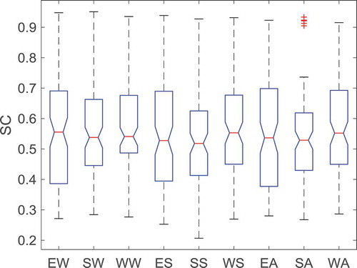
For the comparison of shading performance of east, south and west facades, annual average SC values and seasonal SC values are presented in Figure 3. It can be seen that all these SC values range from about 0.3 to 0.9, indicating a significant fluctuation. Meanwhile, one-way analysis of variance (ANOVA) was conducted to determine whether there are differences between seasons and orientations. The results show that no significant difference can be observed, from the statistical point of view, with the F factor of 1.14 and p value of 0.3337 (higher than the threshold value of 0.05). This means shade stochastic behavior follows similar trends (SC values) for different seasons and orientations.

Figure 3. Seasonal average SC values for east, south and west facades (EW: east winter, SW: south winter, WW: west winter, ES: east summer, SS: south summer, WS: west summer, EA: east annual, SA: south annual, WA: west annual).

3.2. Energy demand

To determine the distribution of annual cooling, heating and total energy data, the normal probability plot was used to graphically compare the distribution of these data to the normal distribution, which is represented by a straight line. If the data are normally distributed, the points in this plot will approximately lie on/near the straight line. Figure 4 gives a normal probability plot of energy data points for cooling, heating and total for east, south and west facades. It can be seen that annual cooling, heating and total energy data all lie on/near the straight line, indicating that the annual heating/cooling and total demands are normally distributed. Furthermore, a more rigorous statistical test of normality of these energy data points was conducted by Shapiro–Wilk test (Razali and Wah 2011). The null-hypothesis of this test is that the data are normally distributed. The results show that these p-values are all higher than 0.05, indicating the null hypothesis cannot be rejected and the energy data points follow normal distributions.

Furthermore, the Kruskal–Wallis test, a nonparametric version of classical one-way ANOVA, was used to determine if the energy data points for different seasons and orientations come from the same population (or the same distribution). This is because ANOVA is not suitable for this analysis due to the violation of the assumption that the energy data points follow normal distributions. The result (p value less than 0.05) shows that there is a significant difference between these different groups of energy data, indicating energy performance differs largely among seasons and orientations. This conclusion can also be easily identified from Figure 5, which shows the box plot of these different groups of energy data points. In addition, it can be seen that east and west facades have a higher energy demand than the south facade, indicating that the same size of window leads to a lower energy demand on the south facade and thus it is better to design large windows on this facade rather than east and west ones.

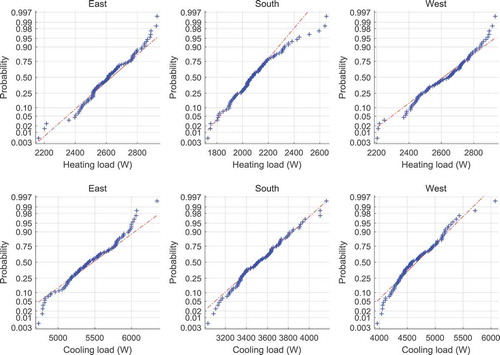
The peak cooling and heating load distributions of the 100 simulation runs for east, south and west facades are illustrated in Figure 6. Compared to annual energy demand, peak energy data does not follow normal distributions since Shapiro–Wilk test shows that some of these p values are less than 0.05. Thus, the following analysis for the required minimum number of simulation runs for determining peak cooling/heating loads cannot be accomplished by using equations described in section 2.3.

Figure 4. Normal probability plot of annual heating, cooling and total energy distributions of the 100 simulation runs for east, south and west facades.

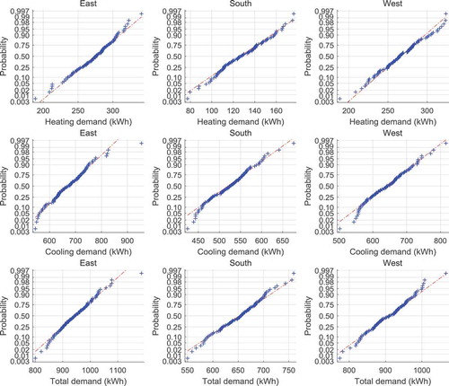
Figure 5. Energy demands for different seasons and different orientations (EW: east winter, SW: south winter, WW: west winter, ES: east summer, SS: south summer, WS: west summer, EA: east annual, SA: south annual, WA: west annual).

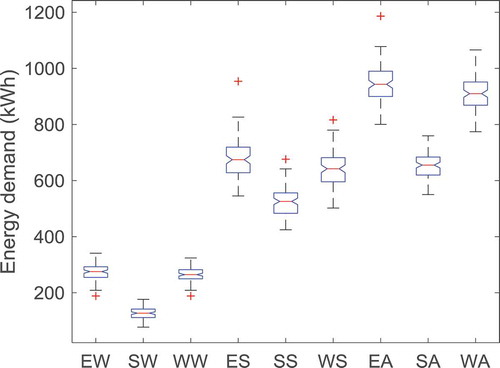
Figure 6. Normal probability plot of peak cooling/heating load distribution of the 100 simulation runs for east, south and west facades.

3.3. Energy uncertainty level

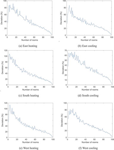
Section 3.2 has shown that energy performance varies among different simulation runs. To determine the energy uncertainty level at different building scales for these three orientations and different seasons, Figure 7 shows a comparison of the energy uncertainty for different orientations and energy types. It can be seen that as the number of rooms increases, cooling, heating and total energy uncertainties decrease significantly from about 25%-60% to about 2%-4%, and for 1–30 rooms there is a sharp decrease while after 50 rooms the energy uncertainty drops to a relatively stable value (around 2–4% depending on orientations and energy types), indicating that for a single room or small office buildings it is important to consider energy uncertainty due to stochastic shade behavior, while there is a relatively small impact of manual shades on energy performance for large buildings.

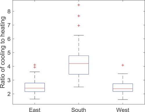
For the cooling and total energy, the trend for different orientations is similar. While for the heating energy, the south facade has a higher uncertainty than east and west facades. In general, heating uncertainty ranks highest, followed by cooling and total energy. This is because the absolute amount of heating energy is much less than cooling energy, which can be seen in Figure 8, and the same amount of variation in heating energy leads to a higher percentage uncertainty than cooling energy. Thus, stochastic shade behavior has a higher impact on uncertainty of heating energy performance and heating performance is more sensitive to occupant behavior than cooling.

Figure 7. Energy uncertainty for different orientations and energy types.

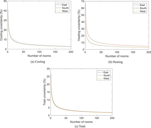
Figure 8. Ratio of cooling energy to heating energy for different orientations.

3.4. Required simulation runs

3.4.1. Annual heating, cooling and total energy demands

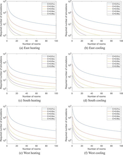
Figure 9 shows the minimum number of required simulation runs for representing reliable annual energy performance for different building scales and accuracy levels. It can be seen that at single or double room scale the required number varies largely depending on required accuracy levels. In this figure, C = 0.01 u represents a 99% prediction accuracy. For a 5% deviation (C = 0.05 u), this number can be less than 30. While for a 1% deviation, this number increases to more than 1000 for south heating and there is a big difference among orientations. Therefore, the computation time and effort are costly for a high accuracy energy prediction at room scale and different orientations cannot be considered equally.

However, this number reduces significantly to lower than 30 as the number of rooms increases to over 20 for all energy types, orientations and accuracy levels. For example, for a 100-room building, this number is only about 1.5 for an accuracy level of 99% and is only 1 if accuracy levels are lower than 99%. The calculated number according to Equation 7(7) $n\ge {\left(\frac{{\mu }_{\alpha /2}\sigma }{C}\right)}^2$(7) ) can be less than 1 as the number of room increases to a certain value. However, the actual number of simulation runs cannot be less than 1 and thus 1 was used instead if calculated number was less than 1 (the minimum number of simulations was 1 as can be seen in Figure 9). In China, most office buildings are high-rise ones with room numbers over 30, and thus a single simulation run is enough to obtain reliable annual heating, cooling and total energy demands (which is not illustrated in this figure but has similar trend as cooling) of office buildings with manual shades, indicating the uncertainty of manual shade adjustment on annual energy performance can be ignored at building scale.

Figure 9. Number of required simulation runs for obtaining reliable annual energy performance at different building scales and accuracy levels.

3.4.2. Peak heating and cooling loads uncertainty

For the peak heating/cooling loads, the uncertainty is also significant, which can be seen from Figure 6. For example, to illustrate the considerable variation of peak loads, Figure 10 presents the maximum deviation of cooling and heating loads from two single simulation runs. It can be seen that as the number of rooms increases the deviation rises to its highest value (over 100%) at around 5–15 rooms and then gradually reduces to less than 3% (for a 100-room building). The interesting finding from this figure is that the maximum deviation does not occur at single room level but at 5–15 rooms. This is mainly due to the fact that the peak loads do not occur at the same time step (e.g. the peak load for one room was at 3 pm July 27th, while another room was at 2 pm July 25th) for different simulation runs due to stochastic nature of occupant behavior, and thus as the number of room increases some cases may have peak values of remaining at around single room level (e.g. the occurred time of peak load was different for each room and thus the peak load is equal to that of a single room which has the maximum value) while some cases may have peak values of being equal to around the sum of these rooms (e.g. 10 rooms have the same occurred time of peak load for one case and 30 rooms for another case), leading to a bigger deviation than at room level. However, as the number of room continues to increase this deviation will diminish due to the smoothing and averaging effect. Therefore, it is important to conduct multiple simulation runs to reduce this uncertainty for a building scale less than 100 rooms.

Figure 10. Maximum deviation of cooling and heating load from two single simulation runs.

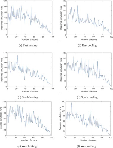
According to section 2.4, random sampling techniques were used to calculate the probability of obtaining peak heating/cooling load at different numbers of simulation runs (see Figure 11). The number of rooms increases as the curves close to the left upper corner of each sub-figure. In general, the larger the building the higher probability to obtain peak heating/cooling load at similar number of simulations, except the cases (5–15 rooms) as described above, which have a lower probability than a single room. To have a better interpretation of this figure, a horizontal line at the y-axis of 95% (represent a 95% probability) can be drawn and the interaction points with the curves can be obtained and are illustrated in Figure 12, which shows the required simulation runs for obtaining reliable peak cooling and heating loads. The curve in this figure has a similar trend as that in Figure 10. It can be seen that peak cooling/heating loads cannot be obtained by a single simulation run even at a 100-room scale and the highest number can be over 120 simulation runs. Therefore, the conclusion for peak loads is different from annual energy demand for a whole building and at least five simulation runs are required to obtain peak heating/cooling loads at building scale. For a smaller building, 120 simulation runs are suggested for peak load determination.

Figure 11. Probability of obtaining peak heating/cooling load at different numbers of simulation runs.

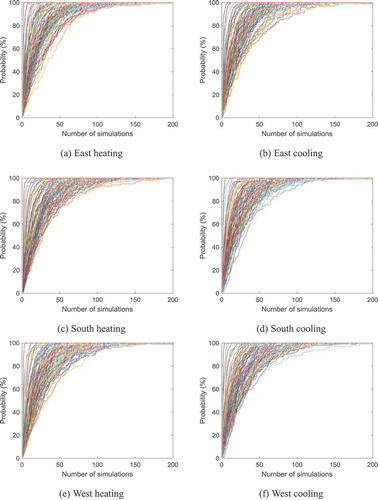
Figure 12. Required simulation runs for obtaining peak cooling and heating loads.

4. Conclusion

This paper investigates the impact of uncertainty of manual solar shades on energy performance. Shading performance, annual heating, cooling and total energy demands were compared between the three orientations at different building scales as well as peak heating/cooling loads. Due to stochastic nature of manual shades, required minimum simulation runs for obtaining reliable annual energy performance and peak loads were calculated based on statistical analysis and random sampling techniques. The following conclusions can be made:

1. Statistical test shows that there is no significant difference in shading performance during different seasons between the three orientations.

2. Annual heating, cooling and total energy demands follow normal distributions while peak heating/cooling load does not. Although shading performance is similar among different orientations, statistical test shows that energy demands differ largely between these orientations. And it is better to design large window on the south facade rather than east and west ones. In addition, heating performance is more sensitive to occupant behavior than cooling.

3. Energy uncertainty levels are high at room scale and drop quickly as the number of rooms increases for different energy types and orientations. In China, most newly built office buildings are high-rise ones and thus the influence of manual shades on the energy uncertainty of these office buildings can be neglected.

4. For large office buildings, a single simulation run is enough to obtain reliable annual heating, cooling and total energy demands. While for peak heating/cooling loads, the conclusion is different from annual energy demand and at least five simulation runs are required to obtain peak heating/cooling loads at building scale. For a smaller building, 120 simulation runs are suggested for peak load determination.

However, the above conclusions are obtained based on the shade behavior model developed in a glazing curtain building in hot summer and cold winter zone of China. There are some limitations to the current research. First, it only includes one type of occupant behavior (i.e. roller shade adjustment, other occupant behaviors such as light switching, window opening were not considered). Second, behavior diversity among occupants was not included in this paper. Third, the shade behavior model was developed based only on one type of buildings (office buildings). In addition, the case study was simulated based on building energy standards in this climate region. Therefore, the energy uncertainty at annual scale was found to be limited and the results may not be directly applicable to other building types and climate regions. Future research efforts are needed to further investigate the potential influence of these factors on shade behavior patterns and energy performance uncertainty.

Acknowledgments

This work was supported by the National Natural Science Foundation of China under Grant No. 51878358, Natural Science Foundation of Zhejiang Province under Grant No. LY18E080012 and National Key Technology R&D Program of the Ministry of Science and Technology under Grant 2013BAJ10B06. The author also would like to thank the K.C.Wong Magna Fund in Ningbo University.

Disclosure statement

No potential conflict of interest was reported by the author.

Additional information

Funding

This work was supported by the National Natural Science Foundation of China [51878358]; Natural Science Foundation of Zhejiang Province [LY18E080012].

Notes on contributors

Jian Yao

Jian Yao is an associate professor at the department of architecture of Ningbo University. Dr. Yao has many years of experience in studying solar shading performance, daylighting and occupant behavior.

References

- Andersen R, V., B. Olesen, and J. Toftum. 2007. “Simulation of the Effects of Occupant Behaviour on Indoor Climate and Energy Consumption.” In Proceedings of Clima 2007 WellBeing Indoors. FINVAC, Helsinki, Finland.
- Andersen, R., V. Fabi, J. Toftum, S. P. Corgnati, and B. W. Olesen. 2013. “Window Opening Behaviour Modelled from Measurements in Danish Dwellings.” Building and Environment 69: 101–113. doi:10.1016/j.buildenv.2013.07.005.
- Azar, E., and C. C. Menassa. 2012. “Agent-Based Modeling of Occupants and Their Impact on Energy Use in Commercial Buildings.” Journal of Computing in Civil Engineering 26 (4): 506–518. doi:10.1061/(ASCE)CP.1943-5487.0000158.
- Chapman, J., P. Siebers, and D. Robinson. 2018. “On the Multi-agent Stochastic Simulation of Occupants in Buildings.” Journal of Building Performance Simulation 11 (5): 604–621. doi:10.1080/19401493.2017.1417483.
- Clevenger, C. M., and J. Haymaker. 2006. “The Impact of the Building Occupant on Energy Modeling Simulations.” In Proc., Joint Int. Conf. On Computing and Decision Making in Civil and Building Engineering. Reston, VA: ASCE.
- Correia Da Silva, P., V. Leal, and M. Andersen. 2013. “Occupants Interaction with Electric Lighting and Shading Systems in Real Single-occupied Offices: Results from a Monitoring Campaign.” Building and Environment 64: 152–168. doi:10.1016/j.buildenv.2013.03.015.
- Da Silva, P. C., V. Leal, and M. Andersen. 2012. “Influence of Shading Control Patterns on the Energy Assessment of Office Spaces.” Energy and Buildings 50: 35–48. doi:10.1016/j.enbuild.2012.03.019.
- Delzendeh, E., S. Wu, A. Lee, and Y. Zhou. 2017. “The Impact of Occupants’ Behaviours on Building Energy Analysis: A Research Review.” Renewable and Sustainable Energy Reviews 80: 1061–1071. doi:10.1016/j.rser.2017.05.264.
- Gilani, S., and W. O’Brien. 2018. “A Preliminary Study of Occupants’ Use of Manual Lighting Controls in Private Offices: A Case Study.” Energy and Buildings 159: 572–586. doi:10.1016/j.enbuild.2017.11.055.
- Gilani, S., W. O’Brien, and H. B. Gunay. 2018. “Simulating Occupants’ Impact on Building Energy Performance at Different Spatial Scales.” Building and Environment 132: 327–337. doi:10.1016/j.buildenv.2018.01.040.
- Gunay, H. B., W. O’Brien, and I. Beausoleil-Morrison. 2013. “A Critical Review of Observation Studies, Modeling, and Simulation of Adaptive Occupant Behaviors in Offices.” Building and Environment 70: 31–47. doi:10.1016/j.buildenv.2013.07.020.
- Haldi, F., and D. Robinson. 2010. “Adaptive Actions on Shading Devices in Response to Local Visual Stimuli.” Journal of Building Performance Simulation 3 (2): 135–153. doi:10.1080/19401490903580759.
- Haldi, F., and D. Robinson. 2011. “The Impact of Occupants’ Behaviour on Building Energy Demand.” Journal of Building Performance Simulation 4 (4): 323–338. doi:10.1080/19401493.2011.558213.
- Hong, T., Y. Chen, Z. Belafi, and S. D’Oca. 2018. “Occupant Behavior Models: A Critical Review of Implementation and Representation Approaches in Building Performance Simulation Programs.” Building Simulation 11 (1): 1–14. doi:10.1007/s12273-017-0396-6.
- Lai, D., S. Jia, Y. Qi, and J. Liu. 2018. “Window-opening Behavior in Chinese Residential Buildings across Different Climate Zones.” Building and Environment 142: 234–243. doi:10.1016/j.buildenv.2018.06.030.
- Li, Z., and B. Dong. 2017. “A New Modeling Approach for Short-term Prediction of Occupancy in Residential Buildings.” Building and Environment 121: 277–290. doi:10.1016/j.buildenv.2017.05.005.
- Macdonald, I. A. 2009. “Comparison of Sampling Techniques on the Performance of Monte Carlo Based Sensitivity Analysis.” In Eleventh International IBPSA Conference. Glasgow, Scotland.
- Newsham, G. R. 1994. “Manual Control of Window Blinds and Electric Lighting: Implications for Comfort and Energy Consumption.” Indoor and Built Environment 3 (3): 135–144. doi:10.1159/000463541.
- O’Brien, W., K. Kapsis, and A. K. Athienitis. 2013. “Manually-operated Window Shade Patterns in Office Buildings: A Critical Review.” Building and Environment 60: 319–338. doi:10.1016/j.buildenv.2012.10.003.
- Page, J., D. Robinson, N. Morel, and J.-L. Scartezzini. 2008. “A Generalised Stochastic Model for the Simulation of Occupant Presence.” Energy & Buildings 40 (2): 83–98. doi:10.1016/j.enbuild.2007.01.018.
- Razali, N., and Y. B. Wah. 2011. “Power Comparisons of Shapiro–Wilk, Kolmogorov–Smirnov, Lilliefors and Anderson–Darling Tests.” Journal of Statistical Modeling and Analytics 2 (1): 21–33.
- Reinhart, C. F. 2004. “Lightswitch-2002: A Model for Manual and Automated Control of Electric Lighting and Blinds.” Solar Energy 77 (1): 15–28. doi:10.1016/j.solener.2004.04.003.
- Reinhart, C. F., and K. Voss. 2003. “Monitoring Manual Control of Electric Lighting and Blinds.” Lighting Research\& Technology 35 (3): 243–260. doi:10.1191/1365782803li064oa.
- Ren, X., D. Yan, and C. Wang. 2014. “Air-conditioning Usage Conditional Probability Model for Residential Buildings.” Building and Environment 81: 172–182. doi:10.1016/j.buildenv.2014.06.022.
- Robinson, S. 2014. Simulation: The Practice of Model Development and Use. UK: Palgrave Macmillan UK.
- Soebarto, V. I., and T. J. Williamson. 2001. “Multi-criteria Assessment of Building Performance: Theory and Implementation.” Building and Environment 36 (6): 681–690. doi:10.1016/S0360-1323(00)00068-8.
- Yan, D., T. Hong, B. Dong, A. Mahdavi, S. D’Oca, I. Gaetani, and X. Feng. 2017. “IEA EBC Annex 66: Definition and Simulation of Occupant Behavior in Buildings.” Energy and Buildings 156 (Supplement C): 258–270. doi:10.1016/j.enbuild.2017.09.084.
- Yao, J. 2014. “Determining the Energy Performance of Manually Controlled Solar Shades: A Stochastic Model Based Co-simulation Analysis.” Applied Energy 127 (8): 64–80. doi:10.1016/j.apenergy.2014.04.046.
- Yao, J. 2018a. “Daylighting Performance Of Manual Solar Shades.” Light & Engineering 26 (1): 99–104.
- Yao, J. 2018b. “Modelling and Simulating Occupant Behaviour on Air Conditioning in Residential Buildings.” Energy & Buildings 175: 1–10. doi:10.1016/j.enbuild.2018.07.013.
- Yao, J. 2019. “Energy Uncertainty of Manual Solar Shades for Different Window-to-wall Ratios.” Journal of Asian Architecture and Building Engineering 18 (6): 575–585. doi:10.1080/13467581.2019.1696205.
- Yao, J., D. Chow, and Y. Chi. 2016. “Impact of Manually Controlled Solar Shades on Indoor Visual Comfort.” Sustainability 8 (8): Article number 727. doi:10.3390/su8080727.
- Yao, J., D. H. C. Chow, R.-Y. Zheng, and C.-W. Yan. 2016. “Occupants’ Impact on Indoor Thermal Comfort: A Co-simulation Study on Stochastic Control of Solar Shades.” Journal of Building Performance Simulation 9 (3): 272–287. doi:10.1080/19401493.2015.1046492.
- Yao, J., and R. Zheng. 2019. “Uncertainty of Energy and Economic Performance of Manual Solar Shades in Hot Summer and Cold Winter Regions of China.” Sustainability 11 (20): Article number 5711. doi:10.3390/su11205711.
- Yao, M., and B. Zhao. 2017. “Window Opening Behavior of Occupants in Residential Buildings in Beijing.” Building and Environment 124: 441–449. doi:10.1016/j.buildenv.2017.08.035.
- Yun, G., D. Y. Park, and K. S. Kim. 2017. “Appropriate Activation Threshold of the External Blind for Visual Comfort and Lighting Energy Saving in Different Climate Conditions.” Building and Environment 113: 247–266. doi:10.1016/j.buildenv.2016.11.021.
- Zhu, P., M. Gilbride, D. Yan, H. Sun, and C. Meek. 2017. “Lighting Energy Consumption in Ultra-low Energy Buildings: Using a Simulation and Measurement Methodology to Model Occupant Behavior and Lighting Controls.” Building Simulation 10 (6): 799–810. doi:10.1007/s12273-017-0408-6.