Collision in the expansion joint effects on the seismic behavior of large-scale aqueduct

ABSTRACT

Under earthquake, two beams of the aqueduct’s expansion joint may collide; thus, this will endanger the safety of the structure and even lead to girder falling accident. Quite a few studies of this issue use the simple one-dimensional model, but little takes the collision phenomenon under the action of multi-dimensional earthquake into account. According to the Contact-Impact Problems of large-scale aqueduct under earthquake action between the adjacent beam segments, a three-dimensional contact analysis model has been used to simulate the collision phenomenon. And the response of aqueduct structure collision one-dimensional seismic and multidimensional earthquake is compared; the results reveal that the three-dimensional frictional contact impact finite element model can simulate the real aqueduct structure under seismic pounding effect.

KEYWORDS:

• Aqueduct
• earthquake
• pounding

1. Introduction

The large aqueduct structure is the key component of the Hydro-Junction Project, and its seismic safety is related to the national economy and the people’s livelihood (Wang et al. 2011; Xu et al. 2010; Yun-he and Hou-qun 2003; Wang and Jie 2001). The form of large-scale aqueducts commonly used in engineering practice is often not conducive to earthquake resistance, and there is no specification in the existing design to follow.

Due to creep, uneven settlement, temperature changes, expansion joints are essential, but under the action of earthquake, large-scale aqueduct’s damage is often due to the collision of the adjacent groove in the position of the expansion joints.

In the Loma Prieta earthquake of 1989, the bridge pier partial structure of the China Basin viaduct in California was damaged and the main cause of the damage was the collision of adjacent beams (Priestley, Seible, and Calvi 1996).

In the Southern California 7.5 Lander earthquake of 1992, a road bridge near Los Angeles was damaged. Since the accelerometer had been installed on this bridge before the earthquake occurred, relevant data had been collected. The research revealed that the acceleration time history curve had many “burrs”, which proved the existence of collision phenomena directly (Jankowski, Wilde, and Fujino 2000).

The beam ends of many bridges were damaged by collision in the American North Ridge earthquake of 1994 (Earthquake Engineering Research Institute (EERI) 1995a). While a beam dropping accident occurred in the first approach bridge of the Xiqiaogang Bridge with a main span of 252 m in the Hanshin earthquake of 1995 in Japan (Earthquake Engineering Research Institute (EERI) 1995b).And the Hanshin Earthquake Investigation Report showed that the main cause of the partial structural damage and the upper structure beam drop was the collision at the joint of the bridge.

In the Tangshan earthquake of 1976 in China, the severe beam drops damage of Weihe River caused the earthquake resistance scholars’ attention. They gave many explanations of the earthquake damage phenomenon and they all mentioned the collision effects in different degrees (Lichu 1981). While in the Wenchuan earthquake of 2008 in China (Qiao and Zhao 2008; Guo, Li, and Li 2011; Jie and Guo-qiang 1992; Bi and Hao 2013), bridge support damage and impact damage at both ends of the expansion joint both occurred.

The expansion joint collision under earthquake is a kind of contact problem. The mechanical behavior is very complicated, and the influencing factors are also many and interrelated. So, it is difficult to describe them accurately. The current research is based on many different kinds of contact unit models including linear spring unit model (Bi and Hao 2013), Kelvin model (Maison and Asaik 1990; Jankowski, Wilde, and Fuzino 1998), Hertz model (Chau and Wei 2001; Pantelides and Ma 1998), Hertz-damp model (Chau 2003), and optimized Hertz-damp model (Hunt and Crossley 1975).

The linear spring model is the simplest contact unit, which just consists of one linearly connected spring, and the energy loss produced by the collision in the linear spring model does not take into account. The linear spring damper unit (Kelvin model), which takes into account the loss of energy during the collision, is consisted of a connecting spring and a damper.

In order to simulate the relationship between collision force and deformation during collision more realistically, a nonlinear spring model based on Hertz’s contact law (Hertz model) was proposed by some scholars. Since the Hertz model cannot simulate the energy dissipation during collisions, the Hertz-damp model, which had been used in the field of robotics and multibody systems for collision problems, was introduced into the field of structural collisions by Muthukumar and DesRoches. A combination of nonlinear springs and nonlinear viscous dampers in the new Hertz-damp model was used to simulate collisions while the nonlinear stiffness and the energy loss were counted during the collision.

It was found that most of the energy loss during the collision was dissipated in the approaching process, and a small part of energy loss because of friction occurred in the collision recovery process. Based on this fact, Jankowski proposed another different Hertz-damp model, which was called optimized Hertz-damp model. The energy loss in the collision recovery process was neglected and all the energy loss during the collision was dissipated in the approaching process in the optimized Hertz-damp model. Considering the contact force and contact deformation characteristics of the collision approaching process and the recovery process, respectively, the impact force is calculated.

Furthermore, in order to study any contact collision between bridge decks, Zhu et al. proposed a three-dimensional contact-friction model (Jankowski 2005; Zhu 2001). Zhu et al. also carried out model test on this three-dimensional contact-friction model. The test showed that this collision model could be used to simulate multi-directional collisions.

Therefore, in view of the current research on the collision of the aqueduct in the expansion joints have not been sufficiently investigated, and mostly based on the spatial beam element model to the main point of collision, and three-dimensional non-elastic contact-friction collision research has not yet mentioned.

In this paper, a three-dimensional solid model is used to simulate the seismic collision of the aqueduct.

2. Dynamic analysis model

2.1. Three-dimensional collision model

At present, in the numerical simulation, the contact–collision interface algorithms are dynamic constraint method, distribution parameter method and penalty function method. Due to the validity and simplicity of the penalty function method in the display analysis, it is widely used in numerical calculation. The penalty function limits the penetration from the node to introduce contact force $f_s$ by introducing a contact spring between the slave and the contact surface.

(1) $f_s=k_i{\mathrm{\Delta }}_i$(1)

where ${\mathrm{\Delta }}_i$ is the amount of penetration.

$k_i$ is the contact stiffness factor, which is calculated by the following formula

(2) $k_i=\frac{f{K}_i{A_i}^2}{V_i}$(2)

where, $K_i$, $V_i,A_i$ are the volume modulus, volume, and area of the primary piece of the unit where the primary film is located, respectively, $f$ is the penalty factor of the contact stiffness, the default value is 0.10, and when the value is too large, the calculation may be unstable.

According to the contact force $f_s$ can calculate the maximum frictional force of the node$F_y$.

(3) $F_y=\mu \left|f_s\right|$(3)

where $\mu$ is the friction coefficient, according to the following formula:

(4) $\mu ={\mu }_d+\left({\mu }_s-{\mu }_d\right)e^{c\left|v\right|}$(4)

where ${\mu }_s,{\mu }_d$ are the static friction coefficient and the east friction coefficient, respectively.

V is the relative velocity between the contact surfaces and C is the attenuation coefficient.

2.2. Collision model based on a beam segment element

As a comparison, a collision model under earthquake was established based on the aqueduct beam unit, as shown in Figure 1.The surface “abcd” is defined as the collision surface and k is the collision point. While p is the contact point on the collision surface and its position can be determined by the “abcd” coordinate.

Figure 1. Pounding model

N is the normal direction.

The displacement relationship between point k and point p can be expressed as:

(5) ${\mathrm{\Delta }}_k=X_p-X_k$(5)

The speed relationship between point k and point p can be expressed as:

(6) $V_{kp}=V_k-V_p$(6)

where X_p and X_k denote the coordinate values of point p and point, respectively. V and V_k denote the velocity values of point p and point k, respectively.

The contact unit between k and p consist of a connecting spring, a normal damper and a tangential damper, as shown in Figure 2.

Figure 2. Contact unit diagram

F(z) can be decomposed into normal component and tangential component, as shown in Figure 3.

Figure 3. Normal force diagram

Where the tangential component force F(z)|t has two modes, one is stick and another slide. The judgment condition is shown in Figure 4.

Figure 4. The Stick and Slide judgment diagram

μ_s denotes the coefficient of static friction in the figure.

When sticking, the tangential force is static friction while when sliding, the tangential force becomes sliding friction force. The collision force of point k can be expressed as:

(7) $F_k=\left\{\begin{array}{c}{F}_{\left(z\right)}+F_c{|}_n+F_c{|}_t\\ F_{\left(z\right)}{|}_n+F_c{|}_n+F_f{|}_t\end{array}\right.\begin{array}{c}strick\\ slide\end{array}$(7)

Where:

(8) $F_c{|}_n=-C\times V_{kp}{|}_n$(8)

(9) $F_c{|}_t=-C_t\times V_{kp}{|}_t$(9)

(10) $F_f{|}_t=-{\mu }_k\times \left|F_{\left(z\right)}{|}_n\right|\frac{V_{kp}{|}_t}{\left|V_{kp}{|}_t\right|}$(10)

where μ_k denotes the coefficient of slide friction, and the force of point p is the reaction force of point k. The force of surface “abcd” can be calculated by linear interpolation and then the collision force can be obtained.

3. Example

Figure 5.1a shows an elevational view of a three-span simple aqueduct that is crossing the canyon. The cross section of the aqueduct is shown in Figure 5.1b and the length of the aqueduct body is 28 m. The trough of the support aqueduct body is 14 m high and its cross section is a cylinder with a radius of 0.4 m. The aqueduct and the cover are connected by a plate rubber bearing. Due to creep, sinking, temperature changes and water shrinkage and expansion will produce concentrated stress in the structure, and it also sets 40 mm expansion joints between the adjacent aqueduct bodies.

Figure 5. Aqueduct schematic diagram

3.1. Unit properties, boundary conditions and contact surfaces

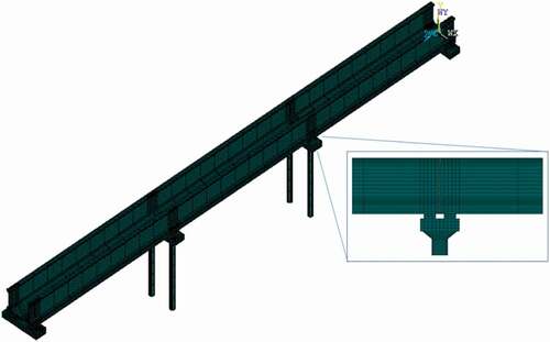
In this paper, all the concrete is an eight-node explicit hexahedral element. Through the optimization of the trial, it is found that the mesh with a size of 200 mm has the same result as the smaller size grid, and the grid with the size of 200 mm uses less computation time. Considering the size of the aqueduct and the locality of the collision under the action of an earthquake, a reasonable grid is only used for the part of the collision. The cell model with a mesh size of 100 mm is only used for the length of 1 m from the slot end. Beyond these areas, the grid has a vertical dimension of 3 m. The rubber mount is modeled using a three-dimensional display structure for solid elements. Figure 6 shows the three-dimensional solid model of the aqueduct.

Figure 6. Aqueduct three-dimensional solid model

3.2. Material model

Table 1 lists the characteristics of the material model used in this paper.

Table 1. Material list

Material	Position	Parameter	Value
Concrete	Aqueduct body collision mesh	Density	2500 kg/m^3
		Compressive strength	25.5 GPa
		Poisson’s ratio	0.3
	Aqueduct body non-collision mesh part	Density	2500 kg/m^3
		Compressive strength	25.5 GPa
		Poisson’s ratio	0.3
	Bent part	Density	2500 kg/m^3
		Compressive strength	25.5 GPa
		Poisson’s ratio	0.3
Rubber bearing	Bearing	Density	2300 kg/m^3
		The bulk modulus	182 MPa
		Fast shear modulus	18.35 MPa
		Slow shear modulus	17.32 MPa
		The attenuation constant	0.153

3.3. Aqueduct beam section element model

The dynamic analysis model based on the aqueduct beam section is shown in Figure 7.

Figure 7. Dynamic analysis model diagram of aqueduct beam section

The stiffness matrix of the aqueduct beam element is derived from the Principle of Potential energy. No.i beam section of the aqueduct elastic strain energy consists of transverse bending strain energy, vertical bending strain energy, longitudinal deformation strain energy, free torsional strain energy, and constrained torsional strain energy. We can calculate the elastic strain energy of No i beam element and take the first variation, and then the element stiffness matrix of the aqueduct beam section can be calculated.

(11) $[K{]}^e=\left[\begin{array}{cccc}{[K_u]}^e& \hspace{0.17em}& \hspace{0.17em}& \hspace{0.17em}\\ \hspace{0.17em}& {[K_v]}^e& \hspace{0.17em}& \hspace{0.17em}\\ \hspace{0.17em}& \hspace{0.17em}& {[K_w]}^e& \hspace{0.17em}\\ \hspace{0.17em}& \hspace{0.17em}& \hspace{0.17em}& \left[K_{\phi }{]}^e+\right[K_w{]}^e\end{array}\right]$(11)

The mass matrix of the aqueduct beam element can be derived from the Principle of total potential energy constant of elastic system dynamics.

(12) $[M{]}^e=\left[\begin{array}{cccc}{[M_{uu}]}^e& \hspace{0.17em}& \hspace{0.17em}& {[M_{u\phi }]}^e\\ \hspace{0.17em}& {[M_{vv}]}^e& \hspace{0.17em}& \hspace{0.17em}\\ \hspace{0.17em}& \hspace{0.17em}& {[M_{ww}]}^e& \hspace{0.17em}\\ {[{M_{\phi }}_u]}^e& \hspace{0.17em}& \hspace{0.17em}& {[M_{\phi \phi }]}^e\end{array}\right]$(12)

The structural damping matrix can be calculated by using the Viscous damping theory. The damping matrix of the aqueduct beam element can be derived from the Principle of the total potential energy constant of the elastic system dynamics.

(13) $[C{]}^e=\left[\begin{array}{cccc}{[C_{uu}]}^e& \hspace{0.17em}& \hspace{0.17em}& {[C_{u\phi }]}^e\\ \hspace{0.17em}& {[C_{vv}]}^e& \hspace{0.17em}& \hspace{0.17em}\\ \hspace{0.17em}& \hspace{0.17em}& {[C_{ww}]}^e& \hspace{0.17em}\\ {[{C_{\phi }}_u]}^e& \hspace{0.17em}& \hspace{0.17em}& {[C_{\phi \phi }]}^e\end{array}\right]$(13)

The water in the tank is simplified according to the Hausner model.

4. Result analysis

4.1. One-dimensional seismic action

The collision response of the three-span simple-support aqueduct structure shown in Figure 5 under earthquake is analyzed in detail by using the dynamic analysis finite element software LS-DYNA. The seismic waves are applied in the longitudinal direction of the aqueduct. The results are shown in Figure 8.

Figure 8. The collision force at the expansion joints

Figure 8 compares the time-course results of the longitudinal impact forces at different expansion joints. As shown in Figure 8, when considering one-dimensional seismic excitation, the times of collisions of adjacent structure in the left, middle 1, middle 2 and the right side of the expansion joints were 10 times, 15 times, 16 times and 11 times, respectively. The maximum impact force is 27.61MN, 23.88MN, 17.16MN and 26.86MN the number of collisions in the middle adjacent groove expansion joints is larger than that of the expansion joints between the two end grooves and the groove body, and the collision force peak is small. This is because when the relative displacement of the trough body and the corresponding trough is greater than the expansion joints, the collision occurs at the left and right ends, and in the middle seam, the determinant of the collision is the relative displacement between the adjacent troughs. Compared with the plat formal trough, because the trough is supported by a flexible bearing, the longitudinal rigidity of the groove body is so small that the trough is more likely to vibrate under the action of the earthquake and produce more collisions. The collision force is relatively small too.

Figure 9 shows the time course of the frictional force in the transverse direction of the expansion joints when considering the three-dimensional contact collision. According to the penalty function, the value of the transverse friction is much smaller than the vertical collision force.

Figure 9. Lateral friction force-time history of expansion joints

Figure 10 is a chart of the vertical longitudinal relative displacement time histogram of adjacent troughs. It can be seen from the figure that when considering the impact of longitudinal relative displacement between adjacent bodies than that without considering the impact is significantly reduced. This is because when a collision occurs in the adjacent groove, a collision force is generated at the collision contact interface, which will result in a decrease in the longitudinal relative displacement of the adjacent groove body. Collision will make the vertical relative displacement of adjacent trough decreases.

Figure 10. Longitudinal relative displacement time histories of adjacent aqueduct body

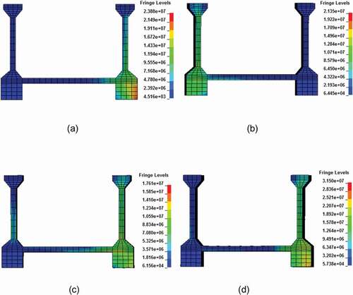
Figure 11 shows the equivalent stress cloud picture of the interface of the expansion joint at the time of collision. It is found from the figure that the equivalent stress value of the bottom plate and the foot of the aqueduct is larger under the effect of one-dimensional longitudinal earthquake, which may cause the local cracking of concrete, thus damage the structure of the aqueduct and affect the aqueduct normal Water supply. And the position of the stress does not change with the collision.

Figure 11. Equivalent stress cloud diagram of collision contact surface under one-dimensional earthquake

4.2. Two-dimensional seismic action

Previous studies of collision responses caused by earthquakes have often only considered longitudinal seismic stimuli. In practice, the spatial variation of the lateral motion and the longitudinal motion simultaneously energize the aqueduct structure, resulting in the aqueduct producing not only a lateral response but also a longitudinal response. Which will lead to collision occurs between the adjacent aqueducts, is not conducive to aqueduct structure earthquake.

Figure 12 compares the results of the time history of longitudinal collision force at each expansion joint under different seismic actions. It can be seen from the above figure that when considering one-dimensional seismic excitation, the peak of the collision force of the adjacent trough structure in the left, middle 1, middle 2 and right ends is 27.61MN, 23.88MN, 17.16MN and 26.86MN, respectively. However, when considering two-dimensional seismic excitation, the corresponding collision force scores are 24.12MN, 19.64MN, 15.21MN and 23.57MN, respectively. One-dimensional seismic incentives can lead to greater impact. This is because, under the action of one-dimensional earthquake, the adjacent structures of the aqueduct will have a face-to-face collision. Under the action of two-dimensional earthquake, the structure responds at the same time in the longitudinal and transverse directions, which will cause the adjacent structures of the aqueduct to oblique impact. In the event of a positive collision, the overall mass of the adjacent troughs is involved in the collision, resulting in a greater impact force due to the resistance to large inertial forces; however, when there is an oblique impact, only part of the mass is involved in the collision One-dimensional seismic excitation has a greater impact force than a two-dimensional seismic stimulus.

Figure 12. Comparison of the time history of the collision force of the expansion joints under one dimension and two-dimensional earthquakes

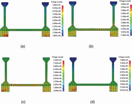
Figure 13 is an equivalent stress cloud picture of the collision contact surface obtained when considering the two-dimensional seismic action. It can be found that when considering the one-dimensional seismic action, the equivalent stress value at the contact surface of each expansion joint is small than one of the equivalent stress values at the corresponding expansion joints considering the two-dimensional seismic action by comparing the equivalent stress cloud images in Figures 11 and 13. This shows that when considering two-dimensional seismic action, the web, flange and bottom plate of the aqueduct will be seriously damaged. It can also be found that the greater collision force between adjacent aqueduct structures does not necessarily lead to greater damage. This is because the damage is related to not only the collision force but also the actual contact surface of each collision. When considering one-dimensional seismic action, the positive impact of the whole surface is produced; in the case of two-dimensional seismic action, the oblique collision of the part is produced. The contact surface under the one-dimensional earthquake is larger than that under the two-dimensional earthquake, so the one-dimensional earthquake produces a large collision force but the damage is smaller.

Figure 13. Equivalent stress cloud diagram of collision contact surface under two-dimensional seismic action

4.3. Results based on aqueduct beam section elements collision

The collision force based on the aqueduct beam section is shown in Figure 14:

Figure 14. The collision force of the left aqueduct expansion joint

It is shown in Figure 14 that the peak value of collision force under one-dimensional collision is bigger than that of two-dimensional collision, which is consistent with the results displayed by the three-dimensional contact model. Under the one-dimensional earthquake input, the collision time of the same expansion joint under two kinds of collision dynamic analysis models is in good agreement. The collision times based on BSE are slightly less than that of the 3D contact analysis model, but the collision force is slightly bigger than the 3D calculation result. Besides comparing Figures 14(b) and Figure 8(b), it can be found that under the two-dimensional earthquake excitation, the three-dimensional contact analysis model has more collisions than the BSE model, and the peak collision force is slightly smaller than BSE model.

The following conclusions can be drawn by comprehensive analysis as follows:

1. The collision occurrence time and the collision force calculation between 3D contact analysis model and collision analysis model-based BSE are very similar, so the calculation result is reliable.

2. The three-dimensional contact analysis model has more collision times than that of BSE-based model. Because considering the shape of the cross-section in the three-dimensional contact analysis model, the contact between the two expansion joints is more frequent. And this is more consistent with reality.

3. The peak collision force of the BSE model is slightly bigger than the three-dimensional contact analysis model. The reason is that when the collision occurs, the cross sections are forced together in the three-dimensional contact analysis mode, so the calculation results of the three-dimensional contact model are more accurate than the BSE dynamic analysis model.

5. Influencing factors analysis

The expansion joint width of the aqueduct influences the collision effect. In order to investigate how different expansion joint width influences the collision effect, different calculation conditions are set for calculation and analysis. Since the aqueduct expansion joint width in the hydraulic engineering is mostly between 3 cm and 5 cm, the design width ranges from 1 cm to 8 cm.

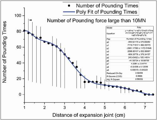
It is seen from Figure 15 that as the width of the expansion joints increases, the number of collisions decreases. After the expansion joint width increases to 7.5 cm, the collision can be avoided. So, the expansion joint width is the key factor to suppress the collision. Besides, when the expansion joint width is small, the occurrence number of the collision force greater than 10 MN is relatively small and this is because a part of the energy is consumed by the frequent collisions.

Figure 15. The relationship between collision times and the expansion joint width

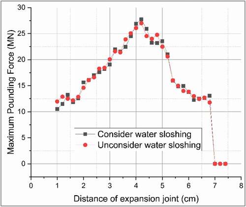
It is seen from Figure 16 that the water shake in the aqueduct has little influence on the collision effect. The reason is that longitudinal water shake is very small compared to the length of the aqueduct body. So, when calculating the collision effect, the aqueduct water shake’s influences can be neglected. Besides, comparing Figure x and Figure 16, the number of collisions will decrease as the width of the expansion joints increases, but the maximum pounding force happens does not reduce when collision occurs.

Figure 16. The aqueduct ‘s water shake influence on the collision effect

6. Conclusion

1. The collision occurrence time and the collision force calculation between 3D contact analysis model and collision analysis model-based BSE are very similar, so the calculation result is reliable.

2. The three-dimensional contact analysis model has more collision times than that of the BSE-based model. Because considering the shape of the cross-section in the three-dimensional contact analysis model, the contact between the two expansion joints is more frequent. And this is more consistent with reality.

3. The peak collision force of the BSE model is slightly bigger than the three-dimensional contact analysis model. The reason is that when the collision occurs, the cross sections are forced together in the three-dimensional contact analysis mode, so the calculation results of the three-dimensional contact model are more accurate than the BSE dynamic analysis model.

4. The use of three-dimensional contact-friction model does not need to assume the location of the collision, which is easy to simulate the face-to-face collision and oblique collision under the multi-dimensional seismic action. It is also possible to obtain the frictional force and stress cloud picture of the contact surface when the adjacent groove is collided and thus clear that the location of the aqueduct is destroyed when the aqueduct collides. Therefore, compared with the previous beam element model, the 3D contact-friction model can simulate the collision response of the large aqueduct structure under the earthquake load factually.

5. Under the action of one-dimensional earthquake and two-dimensional earthquake, the response and damage to large aqueduct structure are different. However, the traditional aqueduct collision response analysis method only takes one-dimensional seismic action into consideration, as a result, it may lead to predictive errors in collision responses and underestimate collision damage. However, under the action of two-dimensional earthquake, although the aqueduct structure only part of the quality involved in the collision and the collision force caused by the smaller inertial resistance will be smaller. However, due to the collision of small contact surface will lead to more serious damage to the aqueduct structure.

6. The water shake in the aqueduct has little influence on the collision effect.

Acknowledgments

This paper is supported by the National Key Research and Development Program of China (2016YFE0205100).

Disclosure statement

No potential conflict of interest was reported by the authors.

Additional information

Funding

This work was supported by the National Key Research and Development Program of China [2016YFE0205100].

Notes on contributors

Liang Huang

Liang Huang received a doctorate degree at ZhengZhou University in 2010, and he has been dedicated to research at ZhengZhou University as a teacher. His main research area is structural engineering.

Yujie Hou

Yujie Hou is a Ph.D. at ZhengZhou University, China. His main research area is structural engineering.

Bo Wang

Bo Wang received a doctorate degree at TongJi University, and he has taught and researched at ZhengZhou University as a research professor. His main research area is structural engineering.

Juncheng Yao

Juncheng Yao is a master student at ZhengZhou University, China. His main research area is structural engineering.

References

- Bi, K., and H. Hao. 2013. “Numerical Simulation of Pounding Damage to Bridge Structures under Spatially Varying Ground Motions.” Engineering Structures 46: 62–76. doi:https://doi.org/10.1016/j.engstruct.2012.07.012.
- Chau, K. T. 2003. “Experimental and Theoretical Simulations of Seismic Poundings between Two Adjacent Structures.” Earthquake Engineering and Structural Dynamics 32 (4): 537 ~ 554. doi:https://doi.org/10.1002/eqe.231.
- Chau, K. T., and X. X. Wei. 2001. “Pounding of Structures Modeled as Non-linear Impacts of Two Oscillators.” Earthquake Engineering and Structural Dynamics 30 (5): 633~651. doi:https://doi.org/10.1002/eqe.27.
- Earthquake Engineering Research Institute (EERI). 1995a. Northridge Earthquake Reconnaissance Report. Rep. No. 95-03. 1995(1), 95-03. Oakland, CA: EERI.
- Earthquake Engineering Research Institute (EERI). 1995b. The Hyogo-ken Nanbu Earthquake of January 17, 1995-preliminary Reconnaissance Report. Rep. No. 95-04. Oakland, CA.
- Guo, A., Z. Li, and H. Li. 2011. “Point-to-surface Pounding of Highway Bridges with Deck Rotation Subjected to Bi-directional Earthquake Excitations.” Journal of Earthquake Engineering 15 (2): 274–302. doi:https://doi.org/10.1080/13632461003739730.
- Hunt, K. H., and F. R. E. Crossley. 1975. “Coefficient of Restitution Interpreted as Damping in Vibrio Impact.” ASME, Journal of Applied Mechanics 42 (2): 440~ 445. doi:https://doi.org/10.1115/1.3423596.
- Jankowski, R. 2005. “Non-linear Viscoelastic Modeling of Earthquake Induced Structural Pounding.” Earthquake Engineering and Structural Dynamics 34 (6): 595–611. doi:https://doi.org/10.1002/eqe.434.
- Jankowski, R., K. Wilde, and Y. Fujino. 2000. “Reduction of Pounding Effects in Elevated Bridges during Earthquakes.” Earthquake Engineering and Structural Dynamics 29 (2): 195–212. doi:https://doi.org/10.1002/(SICI)1096-9845(200002)29:2<195::AID-EQE897>3.0.CO;2-3.
- Jankowski, R., K. Wilde, and Y. Fuzino. 1998. “Pounding of Super Structure Segments in Isolated Elevated Bridge during Earthquakes.” Earthquake Engineering and Structural Dynamics 27 (5): 487~ 502. doi:https://doi.org/10.1002/(SICI)1096-9845(199805)27:5<487::AID-EQE738>3.0.CO;2-M.
- Jie, L., and L. Guo-qiang. 1992. Introduction to Earthquake Engineering. Beijing: Seismological Press.
- Lichu, F. 1981. “Nonlinear Seismic Response Analysis of Beam Bridge: Earthquake Damage Analysis of the Old Luanhe River Bridge.” Journal of Civil Engineering 14 (2): 41–51.
- Maison, B. F., and K. Asaik. 1990. “Analysis for Type of Structural Pounding.” Journal of Structural Engineering, ASCE 116 (4): 957~ 975. doi:https://doi.org/10.1061/(ASCE)0733-9445(1990)116:4(957).
- Pantelides, C. P., and X. Ma. 1998. “L in Ear and Nonlinear Pounding of Structural Systems.” Computers & Structures 66 (1): 79~ 92. doi:https://doi.org/10.1016/S0045-7949(97)00045-X.
- Priestley, M. J. N., F. Seible, and G. M. Calvi. 1996. Seismic Design and Retrofit of Bridge. New York: John Wiley and Sons .
- Qiao, L., and S. Zhao. 2008. Analysis of Seismic Damage of Engineering Structures in Wenchuan Earthquake. Chengdu: Southwest Jiaotong University Press.
- Wang, B., L. Huang, J.-G. Xu, L.-P. Sun, and Y.-J. Hou. 2011. “Analysis of Seismic Response Including Pounding Effect for a Large-Scale Aqueduct.” Journal of Vibration and Shock 30 (4): 265–270.
- Wang, B., and L. Jie. 2001. “Seismic Response Analysis of Large Scale Aqueducts.” China Civil Engineering Journal 34 (3): 29–34.
- Xu, J., B. Wang, H. Chen, and X. Liu. 2010. “Longitudinal Nonlinear Pounding Study of Large-scale Aqueduct under Earthquake.” Earthquake Engineering And Engineering Vibration 30 (5): 126–133.
- Yun-he, L., and C. Hou-qun. 2003. “Aseismic Effect of Lead Rubber Bearing for Large Scaled Aqueduct.” Journal of Hydraulic Engineering 34 (12): 98–103.
- Zhu, P. 2001. “Seismic Analysis and Serviceability Evaluation of Elevated Bridges on 3D Modeling with Pounding Effects of Girders.” Ph. D. Dissertation, University of Tokyo, Tokyo.