An frequency domain analysis method of thermal parameters unsteady-state detection of building wall

ABSTRACT

The in-situ inspection technology of thermal properties of building wall is an important technical guarantee to achieve the goal of building energy conservation. However, there is still a lack of fast, simple, and accurate unsteady-state detection method under natural conditions. This paper focuses on the thermal performance test and analysis method of building wall under natural condition. Two frequency domain analysis methods were developed for the thermal conductivity, as well as volume specific heat and thermal inertia of homogeneous wall along with the harmonic reaction method and the frequency domain analysis theory. The frequency response relationship between the internal and external surface temperature waves and indoor air temperature waves was established, and the relationship contains thermal performance parameters of wall. The thermal conductivity and specific volume heat of wall can be solved by using the response relation. Numerical simulation verification of the method was completed by using ANSYS software and the experimental verification by using wall insulation materials were accomplished in the laboratory. The maximum relative error of numerical simulation results is 1.48%, and that of laboratory experiment results is 8.75%. The implications of these results with respect to the influence on the in-situ inspection technology of building wall are discuss.

KEYWORDS:

• Building envelope
• thermophysical parameters
• in-situ inspection
• unsteady-state
• frequency domain analysis

1. Introduction

When the construction project is completed, the in-situ inspection technology of thermal properties of building wall is an important technical guarantee to achieve the goal of building energy conservation. However, there is still a lack of fast, simple, and accurate unsteady detection method for thermal performance of building wall under natural conditions.

Most of the existing in-situ thermophysical property detection methods of building wall were based on one-dimensional steady-state heat transfer theory. Unsteady-state heat transfer theory has not been effectively applied in the in-situ thermophysical property detection of building wall, and it was more difficult to detect the thermophysical property of building wall in a natural state. Due to the randomness of internal and external disturbance factors in building thermal process, it was difficult to calculate the thermal properties of building wall by using the dynamic test data directly from field tests. Therefore, it was the main technical route of building wall thermal property in-situ test method to artificially create a one-dimensional steady-state detection environment. However, the in-situ test method based on one-dimensional steady-state heat transfer has serious deficiencies in theory and practical application, and its results cannot accurately reflect the real thermal property value of building wall. At the same time, the heat storage parameters of building wall cannot be obtained by one-dimensional steady-state detection method, and the heat storage parameters of building wall is s an important thermophysical parameter to study the thermal process of building.

The heat flow meter method is the authoritative method for measuring the thermal resistance of the building wall structure at home and abroad. For example, it is stipulated in ISO9869 standard “Thermal insulation - Building elements - In-situ measurement of thermal resistance and thermal transmittance” and ASTM C 1155 standard “Standard Practice for Determining Thermal Resistance of Building Wall Components from the In-Situ Data” that thermal transmission properties of the main part of the building wall should be measured by the heat flow meter method. Heat flow meter method is to use heat flow meter and thermocouple in the field to measure the heat flow density and internal and external surface temperature of the measured object, and then calculate its heat transfer coefficient through data processing. However, the defects of the heat flow meter method in field testing include: (1) the temperature difference between indoor and outdoor should be greater than 20°C. (2) To obtain valid data, the test cycle is long. The heat flow meter method requires a one-dimensional steady-state heat conduction process of the building wall. In fact, on the one hand, due to the time delay in the heat transfer process of the building wall, the temperature value and the heat flow value measured at the same time do not coincide in time. On the other hand, in the process of heat transfer from the inside to the outside, there are heat flow components in all directions of the wall, so the heat transfer process of the wall is not one-dimensional (Cha,Seo, and Sumin 2012).

Most of the researches on the unsteady-state detection methods of building wall were carried out in the laboratory. Trethowen (1986) studied the error analysis of pasted heat flow sensor on the wall surface, he predicted the size and relative influence of the error, and also gave the method of selecting heat flow meter for field detection. Bouguerra et al. (Bouguerra and Miri 2001) tested the thermal conductivity, thermal diffusion coefficient and heat capacity of porous building materials by using transient heat source method, and gave the characteristic values of the porous materials, so that the corresponding heat transfer coefficient values of the materials could be obtained through simple calculation.

In addition, the inverse problem method is also used to study the unsteady heat conduction of building wall. Mejias et al. (Mejias, Orlande, and Ozisik 1999) studied the estimation of thermal conductivity using levenberg-marquardt algorithm and conjugate gradient method, and analyzed the measurement accuracy. Huang et al.(Huang and Chen 2000) carried out inverse calculation of thermal conductivity using conjugate gradient method, and verified the correctness by numerical experiments. Engl et al. (Engl and Zhou 2000) studied the regularization method to solve the thermal conductivity, and analyzed the convergence speed. Andrieu et al. (Andrieu and Freitas 2003) promoted the development of the Markov chain Monte Carlo method, which made the Bayesian method begin to be applied to engineering inverse problems. Wang et al. (Wang and Zabaras 2004, 2005a, 2005b) studied the estimation of one-dimensional parameters using Bayesian method. Garcia et al. (Garcia, Scott, and Yvon 1999) applied the genetic algorithm into the study of heat conduction inverse problem and carried out experimental optimization.

The processing of test data is solved by time-domain analysis method in these studies, while the irregular waveform of data shown in time-domain is very difficult to deal with when applied to thermophysical analysis. The accuracy of the solution results depends on the test accuracy of the data.

Unsteady-state methods mainly include numerical analysis method, harmonic reaction method (Mackey and Wright 1946; Gorcum 1951), response factor method (Stephenson and Mitalas 1967,1971; Pederson and Mouen 1973), and z-transfer function (Barakat 1987; Haighight and Sander 1991; Mitalas 1978; Peavy 1978). Due to the theoretical model of building thermal stability established by harmonic response method can reflect the thermal response characteristics of building wall to indoor or outdoor disturbance, and has a clear physical significance for the description of periodic heat transfer process, so it has been widely used to analyze unsteady heat transfer process of building wall.

Based on the theoretical basis of harmonic analysis, the frequency domain analysis method of thermophysical parameters unsteady-state detection of building wall was put forward by converting the problem in time domain to that in frequency domain, that is, some thermophysical parameters are obtained by the relationship between wall thermal system and temperature input/output frequency response, such as thermal conductivity, volume specific heat, index of thermal inertia and so on.

2. Theoretical construction of frequency domain analysis method

2.1. The transfer matrix of the wall thermal system

The unsteady heat transfer process of a single-layer homogeneous wall can be described by the partial differential equation of heat conduction and Fourier law. Its mathematical form is

(1) $\begin{array}{c}\frac{{\mathrm{\partial }}^{2}t(x,\tau )}{\mathrm{\partial }{x}^2}=\frac{1}{a}\frac{\mathrm{\partial }t(x,\tau )}{\mathrm{\partial }\tau }\hspace{0.17em}(0<x<l,\tau >0)\\ q(x,\tau )=-\lambda \frac{\mathrm{\partial }t(x,\tau )}{\mathrm{\partial }x}\hspace{0.17em}(0<x<l,\tau >0)\\ t(x,0)=0\end{array}$(1)

where l is the thickness of the wall; a represents thermal diffusion coefficient, which is equal to$\frac{\lambda }{\rho \cdot c}$; λ, ρ and c represent thermal conductivity, density and mass specific heat.

The transfer matrix of the wall thermal system is obtained by solving Equation (1)(1) $\begin{array}{c}\frac{{\mathrm{\partial }}^{2}t(x,\tau )}{\mathrm{\partial }{x}^2}=\frac{1}{a}\frac{\mathrm{\partial }t(x,\tau )}{\mathrm{\partial }\tau }\hspace{0.17em}(0<x<l,\tau >0)\\ q(x,\tau )=-\lambda \frac{\mathrm{\partial }t(x,\tau )}{\mathrm{\partial }x}\hspace{0.17em}(0<x<l,\tau >0)\\ t(x,0)=0\end{array}$(1) with Laplace transform, as shown in Equation (2)(2) $\left[\begin{array}{c}T(0,s)\\ Q(0,s)\end{array}\right]=\left[\begin{array}{cc}{D}_0(s)& B_0(s)\\ C_0(s)& A_0(s)\end{array}\right]\left[\begin{array}{c}T(l,s)\\ Q(l,s)\end{array}\right]$(2) , which expresses the relationship between the Laplace transforms of temperature and heat flux of the wall inner and outer surface.

(2) $\left[\begin{array}{c}T(0,s)\\ Q(0,s)\end{array}\right]=\left[\begin{array}{cc}{D}_0(s)& B_0(s)\\ C_0(s)& A_0(s)\end{array}\right]\left[\begin{array}{c}T(l,s)\\ Q(l,s)\end{array}\right]$(2)

where $\left[\begin{array}{cc}{D}_0(s)& B_0(s)\\ C_0(s)& A_0(s)\end{array}\right]$ is the transfer matrix of the wall thermal system, represented by G₀. T(0,s) and Q(0,s) represent the Laplace transforms of temperature and heat flux of the wall inner surface. T(l,s) and Q(l,s) represent the Laplace transforms of temperature and heat flux of the wall outer surface.

The total transfer matrix G of single-layer homogeneous wall with the air boundary layer on inner surface is obtained by multiplying the transfer matrix G₀ of the wall and the transfer matrix G_r of air boundary layer on the inner surface, namely

(3) $G=G_0\cdot G_r=\left[\begin{array}{cc}{D}_0(s)& B_0(s)\\ C_0(s)& A_0(s)\end{array}\right]\left[\begin{array}{cc}1& \frac{1}{h_r}\\ 0& 1\end{array}\right]=\left[\begin{array}{cc}D(s)& B(s)\\ C(s)& A(s)\end{array}\right]$(3)

Then the relationship between the Laplace transforms of temperature and heat flux of the outer surface of the wall and the indoor air is as follows

(4) $\left[\begin{array}{c}T(0,s)\\ Q(0,s)\end{array}\right]=\left[\begin{array}{cc}D(s)& B(s)\\ C(s)& A(s)\end{array}\right]\left[\begin{array}{c}T(r,s)\\ Q(r,s)\end{array}\right]$(4)

where T(r,s) and Q(r,s) represent the Laplace transforms of temperature and heat flux of the indoor air.

The relation between the Laplace transform T(l,s) of the inner surface temperature of the wall, the Laplace transform T(0,s) of the outer surface temperature and the Laplace transform T(r,s) of the indoor air temperature can be obtained by solving the systems of simultaneous Equations (2)(2) $\left[\begin{array}{c}T(0,s)\\ Q(0,s)\end{array}\right]=\left[\begin{array}{cc}{D}_0(s)& B_0(s)\\ C_0(s)& A_0(s)\end{array}\right]\left[\begin{array}{c}T(l,s)\\ Q(l,s)\end{array}\right]$(2) , (3(3) $G=G_0\cdot G_r=\left[\begin{array}{cc}{D}_0(s)& B_0(s)\\ C_0(s)& A_0(s)\end{array}\right]\left[\begin{array}{cc}1& \frac{1}{h_r}\\ 0& 1\end{array}\right]=\left[\begin{array}{cc}D(s)& B(s)\\ C(s)& A(s)\end{array}\right]$(3) ) and (4(4) $\left[\begin{array}{c}T(0,s)\\ Q(0,s)\end{array}\right]=\left[\begin{array}{cc}D(s)& B(s)\\ C(s)& A(s)\end{array}\right]\left[\begin{array}{c}T(r,s)\\ Q(r,s)\end{array}\right]$(4) ).

(5) $T(l,s)=\frac{1}{h_{r}B(s)}T(0,s)+\frac{B_0(s)}{B(s)}T(r,s)$(5)

where$\frac{1}{h_{r}B(s)}$is the transfer function of wall inner surface temperature to wall outer surface temperature, and$\frac{B_0(s)}{B(s)}$ represents the transfer function of wall inner surface temperature to indoor air temperature.

Equation (2)(2) $\left[\begin{array}{c}T(0,s)\\ Q(0,s)\end{array}\right]=\left[\begin{array}{cc}{D}_0(s)& B_0(s)\\ C_0(s)& A_0(s)\end{array}\right]\left[\begin{array}{c}T(l,s)\\ Q(l,s)\end{array}\right]$(2) can also be expressed in the following form.

(6) $\left[\begin{array}{c}Q(0,s)\\ Q(l,s)\end{array}\right]=\frac{1}{B_0(s)}\left[\begin{array}{cc}{A}_0(s)& -1\\ 1& -D_0(s)\end{array}\right]\left[\begin{array}{c}T(0,s)\\ T(l,s)\end{array}\right]$(6)

The relation between the Laplace transform Q(l,s) of the inner surface temperature of the wall and the Laplace transform T(l,s) and T(0,s) of the inner and outer surface temperature can be obtained by expanding Equation (6)(6) $\left[\begin{array}{c}Q(0,s)\\ Q(l,s)\end{array}\right]=\frac{1}{B_0(s)}\left[\begin{array}{cc}{A}_0(s)& -1\\ 1& -D_0(s)\end{array}\right]\left[\begin{array}{c}T(0,s)\\ T(l,s)\end{array}\right]$(6) .

(7) $T(l,s)=\frac{1}{D_0(s)}T(0,s)-\frac{B_0(s)}{D_0(s)}Q(l,s)$(7)

where $\frac{1}{D_0(s)}$is the transfer function of wall inner surface temperature to wall outer surface temperature, and$-\frac{B_0(s)}{D_0(s)}$ represents the transfer function of wall inner surface temperature to inner surface heat flux.

2.2. The frequency domain analysis method

Equations (5)(5) $T(l,s)=\frac{1}{h_{r}B(s)}T(0,s)+\frac{B_0(s)}{B(s)}T(r,s)$(5) and (7(7) $T(l,s)=\frac{1}{D_0(s)}T(0,s)-\frac{B_0(s)}{D_0(s)}Q(l,s)$(7) ) respectively express the response relation of wall inner surface temperature when indoor air temperature or heat flux on the inner surface of the wall are taken as input conditions. They can be expressed collectively in the following form.

(8) $T(l,s)=M_k(s)T(0,s)+N_k(s)P_k(s)$(8)

When k = 1, it is named temperature-input method (TIM), $M_k(s)$=$\frac{1}{h_{r}B(s)}$,$N_k(s)$=$\frac{B_0(s)}{B(s)}$,$P_k(s)$= T(r,s).When k = 2, it is called temperature-heat flux input method (TFIM),$M_k(s)$=$\frac{1}{D_0(s)}$, $N_k(s)$=$-\frac{B_0(s)}{D_0(s)}$, $P_k(s)$= Q(l,s).

Generally, in the field test environment, indoor and outdoor temperature are fluctuating. Fourier transform can be used to decompose the temperature of the outer surface of the wall and the heat flux of the room or inner surface into a series of sine functions with integral multiples of frequency, namely harmonic form. Then the temperature waves of the outer surface of the wall and the room temperature are sinusoidal wave forms, whose frequencies are both ω_n, whose amplitudes are A_0n and A_rn, and whose initial phases are φ_0n and φ_rn, where n is the order of the harmoni. The temperature waves of the inner surface of the wall can be expressed in the following formula.

(9) $\begin{array}{c}{t}_{ln}(\tau )={\left\{M_k(i{\omega }_n)A_{0n}{e}^{i({\omega }_n\tau +{\phi }_{0n})}\right\}}_{Im}+{\left\{N_k(i{\omega }_n)A_{kn}{e}^{i({\omega }_n\tau +{\phi }_{kn})}\right\}}_{Im}\\ =A_{0n}\left|M_k(i{\omega }_n)\right|sin({\omega }_n\tau +{\phi }_{0n}-{\psi }_{kn})+A_{kn}\left|N_k(i{\omega }_n)\right|sin({\omega }_n\tau +{\phi }_{kn}-{\chi }_{kn})\end{array}$(9)

where ${\psi }_{kn}$ and ${\chi }_{kn}$ are respectively the argument of the complex number $\frac{1}{M_k(i{\omega }_n)}$ and $\frac{1}{N_k(i{\omega }_n)}$.

To simplify the calculation, assuming$X_n=A_{0n}\left|M_k(i{\omega }_n)\right|,Y_n=A_{kn}\left|N_k(i{\omega }_n)\right|,{\mu }_n={\phi }_{0n}-{\psi }_{kn}$ and${\gamma }_n={\phi }_{kn}-{\chi }_{kn}$, the following formula can be obtained.

(10) $\begin{array}{c}{t}_{ln}(\tau )=X_{n}sin({\omega }_n\tau +{\mu }_n)+Y_{n}sin({\omega }_n\tau +{\gamma }_n)\\ =\sqrt{{X_n}^2+{Y_n}^2+2X_n{Y}_{n}cos({\mu }_n-{\gamma }_n)}\cdot sin({\omega }_n\tau +\theta )\end{array}$(10)

where

$tan\theta =\frac{X_{n}sin{\mu }_n+Y_{n}sin{\gamma }_n}{X_{n}cos{\mu }_n+Y_{n}cos{\gamma }_n}$

Equation (10)(10) $\begin{array}{c}{t}_{ln}(\tau )=X_{n}sin({\omega }_n\tau +{\mu }_n)+Y_{n}sin({\omega }_n\tau +{\gamma }_n)\\ =\sqrt{{X_n}^2+{Y_n}^2+2X_n{Y}_{n}cos({\mu }_n-{\gamma }_n)}\cdot sin({\omega }_n\tau +\theta )\end{array}$(10) expresses the temperature response of the inner surface of the wall under the combined action of the temperature wave on the outer surface of the wall and the indoor temperature wave or the heat flux wave on the inner surface. As can be seen from Equation (10)(10) $\begin{array}{c}{t}_{ln}(\tau )=X_{n}sin({\omega }_n\tau +{\mu }_n)+Y_{n}sin({\omega }_n\tau +{\gamma }_n)\\ =\sqrt{{X_n}^2+{Y_n}^2+2X_n{Y}_{n}cos({\mu }_n-{\gamma }_n)}\cdot sin({\omega }_n\tau +\theta )\end{array}$(10) , the temperature response of the inner surface of the wall is also a sine wave, and the frequency is consistent with the frequency of the temperature of the outer surface of the wall and the indoor air temperature. Therefore, the temperature wave of the inner surface of the wall is expressed as follows.

(11) $t_{ln}(\tau )=A_{ln}sin({\omega }_n\tau +{\phi }_{ln})$(11)

where A_ln and φ_ln Aln are the amplitude and initial phase of the inner surface temperature wave. The theoretical calculation formula of frequency domain analysis method can be obtained by combining Equations (11)(11) $t_{ln}(\tau )=A_{ln}sin({\omega }_n\tau +{\phi }_{ln})$(11) and (10(10) $\begin{array}{c}{t}_{ln}(\tau )=X_{n}sin({\omega }_n\tau +{\mu }_n)+Y_{n}sin({\omega }_n\tau +{\gamma }_n)\\ =\sqrt{{X_n}^2+{Y_n}^2+2X_n{Y}_{n}cos({\mu }_n-{\gamma }_n)}\cdot sin({\omega }_n\tau +\theta )\end{array}$(10) ), namely

(12) $\left.\begin{array}{c}{A_{ln}}^2={X_n}^2+{Y_n}^2+2X_n{Y}_{n}cos({\mu }_n-{\gamma }_n)\\ tan{\phi }_{ln}=\frac{X_{n}sin{\mu }_n+Y_{n}sin{\gamma }_n}{X_{n}cos{\mu }_n+Y_{n}cos{\gamma }_n}\end{array}\right\}$(12)

where λ, C, h_r, A_0n, A_ln, A_kn, φ_0n, φ_ln and φ_kn are independent parameters in Equation (12)(12) $\left.\begin{array}{c}{A_{ln}}^2={X_n}^2+{Y_n}^2+2X_n{Y}_{n}cos({\mu }_n-{\gamma }_n)\\ tan{\phi }_{ln}=\frac{X_{n}sin{\mu }_n+Y_{n}sin{\gamma }_n}{X_{n}cos{\mu }_n+Y_{n}cos{\gamma }_n}\end{array}\right\}$(12) , the thermal inertia index D and coefficient of heat accumulation S are the combined parameters,$D=l\sqrt{\frac{{\omega }_n}{a}}$ and $S=\lambda \sqrt{\frac{{\omega }_n}{a}}$. λ, C, D and S can be solved by using the relationship among nine parameters and the independent parameter values available. The application steps of frequency domain analysis method are as follows:

1. The hourly temperature of the inner and outer surface of the wall and the indoor air as well as the hourly heat flux of the inner wall surface are monitored in a certain period.

2. The parameters A_0n, A_ln, A_kn, φ_0n, φ_ln and φ_kn are obtained by decomposing temperature and heat flux data into harmonic form.

3. The heat transfer coefficient of internal surface h_r is estimated.

4. By substituting the seven parameters obtained in steps (2) and (3) into Equation (12)(12) $\left.\begin{array}{c}{A_{ln}}^2={X_n}^2+{Y_n}^2+2X_n{Y}_{n}cos({\mu }_n-{\gamma }_n)\\ tan{\phi }_{ln}=\frac{X_{n}sin{\mu }_n+Y_{n}sin{\gamma }_n}{X_{n}cos{\mu }_n+Y_{n}cos{\gamma }_n}\end{array}\right\}$(12) and turning it into a binary nonlinear equation set, the thermal conductivity λ and volume specific heat C of single-layer wall or thermal inertia index D and coefficient of heat accumulation S of multi-layer wall are obtained by solving it. Where n = 1.

The assumed condition of Equation (12)(12) $\left.\begin{array}{c}{A_{ln}}^2={X_n}^2+{Y_n}^2+2X_n{Y}_{n}cos({\mu }_n-{\gamma }_n)\\ tan{\phi }_{ln}=\frac{X_{n}sin{\mu }_n+Y_{n}sin{\gamma }_n}{X_{n}cos{\mu }_n+Y_{n}cos{\gamma }_n}\end{array}\right\}$(12) in the derivation process is single-layer homogeneity. Since the total thermal inertia index of multi-layer wall is the sum of the thermal inertia index of each constituent layer, which is independent of the sequence of each constituent layer, when solving the thermal performance of multi-layer wall, multi-layer wall can be regarded as a whole, and the overall thermal inertia index can be obtained by the idea of solving the thermal inertia index of single-layer wall. Another parameter solved is the overall coefficient of heat accumulation. When the order of structure of the multi-layer wall changes, the overall thermal inertia index remains unchanged, while the overall coefficient of heat accumulation changes, but for the existing multi- layer building wall, the composition of each layer is fixed, whose resistance to temperature waves is constant, so the overall coefficient of heat accumulation is able to reflect the unsteady heat transfer characteristics of the existing wall. In this paper, the overall coefficient of heat accumulation is expressed as characteristic value of heat accumulation S ‘.

3. Simulation verification

3.1. Simulation verification for single-layer materials

3.1.1. The research objects

Sintered shale brick (Material 1), thermal insulation mortar (Material 2) and custom material (Material 3) were taken as research objects. The thermal conductivity of the custom material is the same as that of Material 1, and the specific heat of volume is the same as that of Material 2. The thermophysical parameters of the three materials are shown in Table 1.

Table 1. The thermophysical parameters of the simulated object

Material	λ (W m^−1 K^−1)	ρ (Kg m^−3)	c (kJ kg^−1 K^−1)	C (kJ m^−3 K^−1)
Sintered shale brick	0.87	1800	1.06	1908
Thermal insulation mortar	0.29	800	1.05	840
The custom material	0.87	800	1.05	840

3.1.2. Conditions set

The single-layer wall models of Materials 1, 2 and 3 were established in ANSYS software, with the thickness taken as 120 mm, and the boundary conditions were set as follows. The temperature of the outer surface of the wall and the air layer on the inner surface were non-standard sinusoidal waves with a period of 24 hours. The heat transfer coefficient of internal surface was 8.7 W/(m²·K). The simulation time was 72 hours for three cycles, and the time step length was 1 minute. The monitoring points of temperature and heat flux are set on the inner surface of the wall.

3.1.3. Results and analysis

The temperature and heat flux data obtained from three groups of monitoring simulation results is shown in Figure 1.

Figure 1. Temperature and heat flux curves at monitoring points of the three materials over time

As can be seen from Figure 1, the temperature and heat flux in the three simulated groups did not reach the stable periodic change state in the first cycle because the temperature distribution in the wall had an initial state at the beginning of the calculation, which would affect the periodic heat transfer process in a certain period of time after the calculation began. Therefore, in order to eliminate the influence of the temperature distribution in the initial state on the calculation results, the simulation time was set as three cycles, and the data of the last cycle was taken for analysis and calculation. The amplitude and initial phase of first-order harmonics of temperature and heat flux on the inner surface are obtained by harmonic decomposition of each group of temperature and heat flux data, as shown in Table 2.

Table 2. Amplitude and initial phase of first-order harmonics of temperature and heat flux at each monitoring point of the three materials

Material	Amplitude		Initial phase
	Inner surface temperature (°C)	Inner surface heat flux (W m^−2)	Inner surface temperature (rad)	Inner surface heat flux (rad)
1	5.7176	15.5580	−0.8908	2.4907
2	4.7454	6.4562	−0.9976	2.1518
3	6.0654	25.2313	−0.5802	−3.1308

The thermal conductivity, volume specific heat and relative errors of the three materials were calculated by Equation (12)(12) $\left.\begin{array}{c}{A_{ln}}^2={X_n}^2+{Y_n}^2+2X_n{Y}_{n}cos({\mu }_n-{\gamma }_n)\\ tan{\phi }_{ln}=\frac{X_{n}sin{\mu }_n+Y_{n}sin{\gamma }_n}{X_{n}cos{\mu }_n+Y_{n}cos{\gamma }_n}\end{array}\right\}$(12) , as shown in Table 3.

Table 3. Thermal conductivity, volume specific heat and relative errors of three materials calculated by the two methods

Material	TIM				TFIM
	λ (W m^−1 K^−1)	C (kJ m^−3 K^−1)	Δλ (%)	ΔC (%)	λ (W m^−1 K^−1)	C (kJ m^−3 K^−1)	Δλ (%)	ΔC (%)
1	0.8595	1883.7369	1.2069	1.2717	0.8572	1881.1029	1.4713	1.4097
2	0.2870	831.2220	1.0345	1.0450	0.2857	828.9543	1.4828	1.3150
3	0.8661	832.9387	0.4483	0.8406	0.8642	834.1278	0.6667	0.6991

The results in Table 3 show that the relative errors of the thermal conductivity and volume specific heat of the three materials calculated by the two methods are all less than 1.5%, and are calculated errors. This shows that the two methods proposed in this paper are feasible and theoretically correct under the assumed heat transfer conditions.

It can be seen from Figures 1 to 3 that under the action of temperature waves in the air layer on the same outer and inner surfaces, although the thermal conductivity of Material 3 and Material 1 is the same, the temperature response of the inner surface is also different due to the different volume specific heat of the two materials. Even though the specific heat of the volume of Material 3 and Material 2 is the same, the temperature response of the inner surface is different due to the different thermal conductivity of the two materials. Since the thickness of Material 3 and Material 1 is the same, the thermal resistance is the same and the thermal response is different, indicating that the thermal resistance alone cannot fully evaluate the thermal performance of the wall.Figure 2.

Figure 2. Six walls formed by three materials in six sequences

Figure 3. Single homogeneous material tested

Comparing the data of Material 1 and Material 3 in Table 2, it can be shown that in the case of the same thermal conductivity, the larger the specific heat of the material, the greater the attenuation factor of the temperature wave on the outer and inner surfaces of the material, and the longer the delay time. Comparing the data of Material 2 and Material 3, it can be seen that in the case of the same volume specific heat, the greater the thermal conductivity of the material, the smaller the attenuation factor of the temperature wave of the material’s internal and external surface, and the shorter the delay time. Therefore, the frequency response characteristics of the materials are determined by the thermal conductivity and specific heat of volume.

3.2. Simulation verification of multilayer wall

3.2.1. The research objects

For multi-layer walls, in addition to verifying the accuracy of solving the overall thermal inertia index by the frequency domain analysis methods, it is also necessary to verify the sequence independence of each layer of the wall. In order to make the thermophysical parameters of each material layer different, the thermophysical parameters of custom Material 4 are set as follows. The thermal conductivity is 0.5 W/(m·K).The density is 1500 kg/m³. The mass specific heat is 1.02 kJ/(kg·K). The volume specific heat is 1530 kJ/(m³·K).

The multi-layer wall composed of Materials 1, 2 and 4 is taken as the research object. The thickness of each material layer is 60 mm (Material 1), 20 mm (Material 2) and 40 mm (Material 4). The height is 500 mm and the total wall thickness is 120 mm. According to Equations (5)(5) $T(l,s)=\frac{1}{h_{r}B(s)}T(0,s)+\frac{B_0(s)}{B(s)}T(r,s)$(5) and (6(6) $\left[\begin{array}{c}Q(0,s)\\ Q(l,s)\end{array}\right]=\frac{1}{B_0(s)}\left[\begin{array}{cc}{A}_0(s)& -1\\ 1& -D_0(s)\end{array}\right]\left[\begin{array}{c}T(0,s)\\ T(l,s)\end{array}\right]$(6) ), it can be calculated that the thermal inertia index of multi-layer wall composed of three materials is 1.6447. To obtain six types of multi-layer wall a ~ f, the material layers are arranged in the order of a, b, c, d, e and f, as shown in

3.2.2. Results and analysis

The setting of simulation conditions is the same as in Section 2.1.2. Similarly, the Fourier transform is used to obtain the amplitude and initial phase of the first harmonic from the extracted inner surface temperature and heat flux, as shown in Table 4.

Table 4. Amplitude and initial phase of first-order harmonics of temperature and heat flux at monitoring points of the wall a ~ f

Wall	Amplitude		Initial phase
	Inner surface temperature (°C)	Inner surface heat flux (W m^−2)	Inner surface temperature (rad)	Inner surface heat flux (rad)
a	4.9144	7.9878	−0.9749	2.2759
b	4.7505	6.5852	−0.9737	2.3022
c	5.3340	11.6957	−0.9563	2.3132
d	5.1369	9.9344	−0.9682	2.2820
e	5.4447	12.5445	−0.9816	2.2089
f	4.8504	7.4421	−0.9741	2.2845

The thermal inertia index, characteristic value of heat accumulation and their relative errors of the six walls are calculated by using Equation (12)(12) $\left.\begin{array}{c}{A_{ln}}^2={X_n}^2+{Y_n}^2+2X_n{Y}_{n}cos({\mu }_n-{\gamma }_n)\\ tan{\phi }_{ln}=\frac{X_{n}sin{\mu }_n+Y_{n}sin{\gamma }_n}{X_{n}cos{\mu }_n+Y_{n}cos{\gamma }_n}\end{array}\right\}$(12) , as shown in Table 5.

Table 5. Thermal inertia index, characteristic value of heat accumulation and relative error of wall a ~ f calculated by the two methods

Wall	TIM			TFIM
	D	S′ (W m^−2 K^−1)	ΔD (%)	D	S′ (W m^−2 K^−1)	ΔD (%)
a	1.6799	5.0894	2.1402	1.6810	5.0773	2.2071
b	1.6830	3.8951	2.3287	1.6845	3.8900	2.4199
c	1.6263	8.4589	1.1187	1.6268	8.4332	1.0902
d	1.6560	6.8206	0.6871	1.6567	6.8013	0.7296
e	1.6570	10.4952	0.7479	1.6574	10.4608	0.7722
f	1.6810	4.6000	2.2071	1.6821	4.5912	2.2740

Table 5 shows the calculation results of the two methods under simulated conditions are not different. Compared with the theoretical value, the relative errors of the thermal inertia indexes calculated by the frequency domain analysis methods are less than 2.5%. The thermal inertia index of six kinds of multi-layer walls is basically the same. Therefore, it is feasible to solve the thermal inertia index of multi-layer walls by the frequency domain analysis methods. But the characteristic value of heat accumulation of the six walls is different. Combined with Tables 4 and 5, it can be seen that the characteristic value of heat accumulation and the amplitude of inner surface temperature wave of wall b are the minimum, while the characteristic value of heat accumulation and the amplitude of inner surface temperature wave of wall e are the maximum. The layers of wall b and e are arranged in reverse order. The coefficient of heat accumulation of single-layer Material 1 is 10.987 W/(m²·K), that of Material 2 is 4.209 W/(m²·K), and that of Material 4 is 7.459 W/(m²·K). Material 1 has the largest thermal accumulation coefficient, followed by Material 4, and Material 2 has the smallest thermal accumulation coefficient. Each constituent layer of Wall b is arranged from outside to inside in the order of thermal accumulation coefficient from small to large, while each constituent layer of wall e is arranged in the order of thermal accumulation coefficient from large to small. This shows that the material layer with a small coefficient of thermal accumulation is set on the outside, the overall number of thermal accumulation characteristics is small, and the inner surface of the wall has a large attenuation factor for the outdoor temperature wave. Thermal insulation materials are mostly light materials with small density and small thermal accumulation coefficient. The greater attenuation factor and better thermal insulation performance can be obtained by setting the insulation layer on the outside.

4. Experimental verification and analysis

4.1. Experiment platform

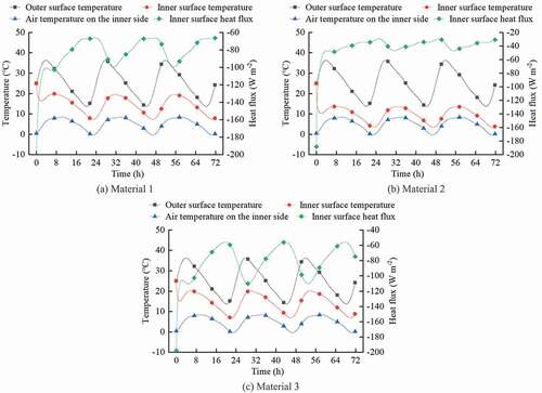
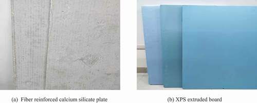
The single-layer homogenous material tested in the experiment is a fiber-reinforced calcium silicate plate (Material 5) with the thicknesses of 7mm and 14 mm, and a XPS extruded plate (Material 6) with the thicknesses of 20 mm and 30 mm, with a length and width of 1 meter, as shown in Figure 4. The thermophysical parameters of the material are shown in Table 6. The multi-layer material is a 135 mm thick wall (Material 7) composed of 115 mm solid brick and 10 mm cement mortar plastering on both sides, which is directly built in the specimen frame of the building wall thermal insulation performance testing device. The photo and its structure are shown in Figure 5. The thermophysical parameters of each component layer are shown in Table 7. For the verification of single-layer wall and multi-layer wall, the experimental process and data acquisition are consistent. The instruments used in the experiment mainly include JTRG-I building wall thermal insulation performance detection device, TR70B field heat transfer coefficient detector, and HFM-4 series heat flux meter. The construction of the experimental platform is shown in

Figure 4. Multilayer material tested

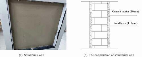
Figure 5. Establishment of the experiment platform

Figure 6. Figure 6.

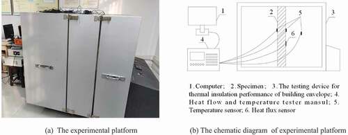
Figure 6. Layout of measuring points

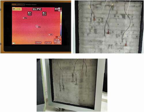
Table 6. The thermophysical parameters of single-layer homogeneous materials

Material	λ (W m^−1 K^−1)	ρ (Kg m^−3)	c (kJ kg^−1 K^−1)	C (kJ m^−3 K^−1)
Fiber-reinforced calcium silicate plate	0.25	1270	1.28	1625.6
XPS extruded plate	0.029	33	1.42	46.86

Table 7. The thermophysical parameters of multilayer materials

Material	Thickness (mm)	λ (W m^−1 K^−1)	ρ (Kg m^−3)	c (kJ kg^−1 K^−1)	D (T = 24h)
Solid brick	115	0.76	1540	1.24	1.555
Cement mortar	10	0.93	1800	1.05	0.122
Solid brick wall	135	–	–	–	1.798

The instruments used in the experiment mainly include two parts. One part is the instrument for the detection of thermal physical frequency-domain analysis method, including JTRG-I insulation performance detecting device of building envelope structure, TR70B field heat transfer coefficient detector, HFM-4 series heat flow meter and TiX560 infrared thermal imager. The other part is the precise experimental instrument for measuring the thermal conductivity and specific heat capacity of the materials, including TC3000E hot-wire thermal conductivity meter and DSC Q2000 differential scanning calorimeter. The performance and technical parameters of each instrument are shown in Tables 8–10.

Table 8. Technical parameters of JTRG-I

Name	Temperature control range	Control accuracy	Power
Hot-box	Ambient temperature ~50°C	±0.2°C	0 ~ 800 W
Cold-box	−10°C~ Ambient temperature	±0.2°C	0.3 KW

Table 9. Technical parameters of TR70B

Instrument	Sensor		Acquisition accuracy	Temperature measuring range
TR70B field heat transfer coefficient detector		Pt1000	±0.1°C	−100.00~+100.00°C

Table 10. Sensitivity coefficient table of HS-30

Instrument model	Size	Operating temperature	Thermal impedance	Electrical impedance	Response time	Accuracy	Sensitivity coefficient Ks[μV/(W/m^2)]
HS-30	30 mmx30mmx0.4 mm	−180 ~ 200°C	0.006 °C/W/m^2	100 Ω/dm^2	0.3s	Better than 3%	#4517 (8.25) #4515 (8.17) #4511 (7.87)

Before arranging the measuring points, the thermal defects of the whole material are detected by an infrared thermal imager to avoid placing the measuring points in places where there are thermal defects such as cracks, voids and thermal bridges inside the material. The heat flow sensor is arranged on the cold side wall surface of the material, and then the temperature sensor is pasted and mounted adjacent to the heat flow sensor. Meanwhile, the temperature sensor is disposed at the corresponding position on the hot side wall surface of the material. Three measuring points are arranged for each measuring object to reduce the accidental error of the measurement. The layout of measuring points is shown in

4.2. Test results and data preprocessing

The testing device for thermal insulation performance of building envelope is equipped with a heating box and a refrigeration box, which are used to construct a test environment with temperature approximately periodic change on both sides of the specimen. Meanwhile, the cold and hot side wall surface temperature, cold side air temperature and the heat flux on the cold side wall surface are monitored and collected. The time-varying curves of the data are shown in Figures 7 and 8.

Figure 7. Curve of temperature and heat flux at each measuring point of single-layer materials over time

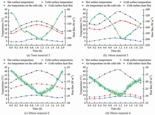
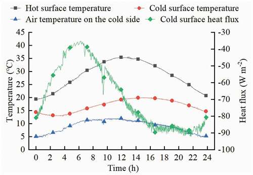
Figure 8. Curve of temperature and heat flux at each measuring point of solid brick wall over time

The amplitude and initial phase of the first harmonic were obtained by decomposing temperature and heat flux data at each measuring point into harmonic form, as shown in Table 11.

Table 11. Amplitude and initial phase of first-order harmonic of temperature and heat flux at each measuring point of the specimen

Material		Amplitude				Initial phase
		Hot surface temperature	Cold surface temperature	Air temperature on the cold side	Cold surface heat flux	Hot surface temperature	Cold surface temperature	Air temperature on the cold side	Cold surface heat flux
5	7 mm	6.0213	5.1917	1.7000	30.8557	−1.5070	−1.6384	−1.7034	1.5338
	14 mm	7.8695	5.3478	1.8120	39.0340	−2.1657	−2.5009	−1.5001	0.3095
6	20 mm	6.3122	2.2597	1.5963	6.5608	−1.7240	−1.5804	−1.3873	1.1316
	30 mm	7.5504	2.2118	1.7120	5.1421	−1.5756	−2.2652	−2.4469	1.3985
Solid brick wall		7.2054	3.3311	3.0693	25.4178	−1.7390	−2.3470	−1.4263	−0.1831

4.3. Calculation results and analysis of single-layer material

The thermal conductivity, volume specific heat and relative errors of the two materials calculated by Equation (12)(12) $\left.\begin{array}{c}{A_{ln}}^2={X_n}^2+{Y_n}^2+2X_n{Y}_{n}cos({\mu }_n-{\gamma }_n)\\ tan{\phi }_{ln}=\frac{X_{n}sin{\mu }_n+Y_{n}sin{\gamma }_n}{X_{n}cos{\mu }_n+Y_{n}cos{\gamma }_n}\end{array}\right\}$(12) are shown in Table 12.

Table 12. Thermal conductivity, volume specific heat and relative errors of two materials calculated by the two methods

Material		TIM				TFIM
		λ (W m^−1 K^−1)	C (kJ m^−3 K^−1)	Δλ (%)	ΔC (%)	λ (W m^−1 K^−1)	C (kJ m^−3 K^−1)	Δλ (%)	ΔC (%)
5	7 mm	0.2673	1749.5910	6.9200	7.6274	0.2711	1776.8605	8.4400	9.3049
	14 mm	0.2381	1540.8233	4.7600	5.2151	0.2311	1490.3615	7.5600	8.3193
6	20 mm	0.0312	42.9817	7.5862	8.2764	0.0308	43.1341	6.2069	7.9511
	30mm	0.0317	50.6669	9.3103	8.1240	0.0307	49.9327	5.8621	6.5572

The results in Table 12 show that the relative error of the thermal conductivity calculated by the temperature input method is 4.5%~9.5%, and that of the volume specific heat is 5%~9.5%; while the relative error of the thermal conductivity calculated by the temperature-heat flux input method is 5.5%~9%, and that of volume specific heat is 6.5%~9.5%, which indicates that the two methods are feasible for detecting the thermal conductivity and volume specific heat of single-layer homogeneous wall. However, compared with the calculation results under simulation conditions, the relative error of the experimental results is larger, all kinds of possible reasons in producing errors of experimental results are analyzed as follows. (1) The formula derivation of the two methods assumes that the heat transfer process is one-dimensional heat transfer. (2) In the experimental test, there will be errors in the measurement of temperature and heat flux. (3) The temperature and heat flux changes under experimental conditions are not standard sinusoidal waves. When using the frequency domain analysis method, only the first-order harmonic is taken as the input condition with the higher order harmonic parts filtered out, thus generating the truncation error of data.

4.4. Calculation results and analysis of  multi-layer  wall

The thermal inertia index, characteristic value of heat accumulation and their relative errors of the six walls are calculated by using Equation (12)(12) $\left.\begin{array}{c}{A_{ln}}^2={X_n}^2+{Y_n}^2+2X_n{Y}_{n}cos({\mu }_n-{\gamma }_n)\\ tan{\phi }_{ln}=\frac{X_{n}sin{\mu }_n+Y_{n}sin{\gamma }_n}{X_{n}cos{\mu }_n+Y_{n}cos{\gamma }_n}\end{array}\right\}$(12) , as shown in Table 13.

Table 13. Thermal inertia index, characteristic value of heat accumulation and relative error of the solid brick wall calculated by the two methods

Method	Calculated value		Relative error
	D	S′/(W/(m^2·K))	ΔD (%)
TIM	1.9550	10.4585	8.7528
TFIM	1.9178	10.9253	6.6835

Table 1 shows that the relative error of thermal inertia index of solid brick wall calculated by temperature input method is about 8.7%, and that of temperature-heat flux input method is about 6.7%, indicating that the two methods are feasible to detect the thermal inertia index of multi-layer wall. Meanwhile, the characteristic values of heat accumulation calculated are 10.4585 and 10.9253, which reflect the heat storage characteristic of the solid brick wall. In addition to the factors mentioned in Section 4.3, another reason for the error of the above experimental results is that there is a certain deviation between the actual thermal properties of the wall and the theoretical values. The process of building the solid brick wall is complex, and the wall quality is affected by subjective and objective factors, such as the error ratio of cement mortar, mortar and solid brick joint degree and so on, which will cause a certain deviation between the actual thermal performance of the wall and the theoretical value of 1.798, resulting in the uncertainty of the real thermal performance of multilayer wall. Relying only on the energy-saving requirements and material selection based on the energy-saving standards during the design stage, it is not possible to grasp the real thermal performance parameters of the wall and completely ensure that the wall meets the requirements of the energy-saving standards after the completion of construction. The detection method proposed in this paper can provide a reference value for the field evaluation of the thermal performance of the wall.

5. Conclusion

Through theoretical derivation, simulation and experimental testing, the frequency-domain analysis method for detecting the thermal physical parameters of walls is investigated in this paper, and some findings of this study can be summarized as follows:

1. Under the condition of simulated heat transfer, the thermal conductivity and volume specific heat of the three monolayer materials were solved by using the thermophysics unsteady frequency domain analysis method, and the relative error was within 1.5%, which verified the correctness of the theory of this method for solving monolayer homogeneous wall. And then under the same initial and boundary conditions, the thermal inertia index and characteristic value of heat accumulation of six wall composed of three kinds of different material layers by six kinds of different order are solved. The calculation results of the two methods have no obvious difference, and the thermal inertia indexes of the six wall are also roughly the same, and the relative error is within 2.5% compared with the theoretical calculation value, indicating that the frequency-domain analysis methods is feasible in theory for solving the thermal inertia indexes of the multi-layer wall.

2. The characteristic values of heat accumulation of six walls with the same material and different order calculated by frequency domain analysis methods are different. The characteristic value of heat accumulation proposed in this paper is consistent with the physical meaning of the coefficient of heat accumulation of the single-layer wall, which reflects the heat storage characteristic of the multi-layer wall under the specific sequence of each constituent layer and specific structure.

3. On the basis of testing experiments for thermophysical parameters of two monolayer homogeneous materials and a solid brick walls with cement plaster on both sides, the thermal conductivity coefficient and volume specific heat of single-layer homogeneous materials and thermal inertia index of solid brick walls were calculated by the unsteady frequency domain analysis methods. The average relative errors of calculation results were less than 10% compared with the actual values, which proves that the methods are feasible to detect the thermophysical parameters of the wall under the condition of unsteady heat transfer.

4. The frequency domain analysis method proposed in this paper is a new unsteady detection technology for building thermal property, which only needs to obtain the temperature and heat flux value, and is not limited by the field environment. Moreover, the testing process is simple, which has certain theoretical significance and engineering application value.

Disclosure statement

No potential conflict of interest was reported by the authors.

References

- Andrieu, C., N. D. Freitas, A. Doucet, M. I. Jordan. 2003. “An Introduction to MCMC for Machine Learning.” Machine Learning 50 (1/2): 5–43. doi:https://doi.org/10.1023/A:1020281327116.
- Barakat, S. A. 1987. “Experimental Determination of the Z Transfer Function Coefficients for House.” ASHRAE Transactions 93 (1): 146–160.
- Cha, J. H., J. K. Seo, and K. Sumin. 2012. “Building Materials Thermal Conductivity Measurement and Correlation with Heat Flow Meter, Laser Flash Analysis and C-Therm TCi.” Journal of Thermal Analysis & Calorimetry 109 (1): 295–300. doi:https://doi.org/10.1007/s10973-011-1760-x.
- Engl, H. W., and J. Zou. 2000. “A New Approach to Convergence Rate Analysis of Tikhonov Regularization for Parameter Identification in Heat Conduction.” Inverse Problems 16 (16): 1907–1923. doi:https://doi.org/10.1088/0266-5611/16/6/319.
- Garcia, S. 1999. Experimental Design Optimization and Thermophysical Parameter Estimation of Composite Materials Using Genetic Algorithms. Virginia Tech. Nantes, FRA.
- Gorcum, A. H. V. 1951. “Theoretical Considerations on the Conduction of Fluctuating Heat Flow.” Applied Scientific Research 2 (1): 272. doi:https://doi.org/10.1007/BF00411989.
- Haighight, F., D. M. Sander, and H. Liang. 1991. “An Experimental Procedure for Deriving Z Transfer Function Coefficients of Building Envelope.” ASHRAE Transactions 97 (2): 90–98.
- Huang, C., and W. Chen. 2000. “A Three-dimensional Inverse Forced Convection Problem in Estimating Surface Heat Flux by Conjugate Gradient Method.” International Journal of Heat and Mass Transfer 43 (17): 3171–3181. doi:https://doi.org/10.1016/S0017-9310(99)00330-0.
- Lu, X., and A. Memari. 2018. “Comparative Study of Hot Box Test Method Using Laboratory Evaluation of Thermal Properties of a Given Building Envelope System Type.” Energy & Buildings 178: 130–139. doi:https://doi.org/10.1016/j.enbuild.2018.08.044.
- Mackey, C. O., and L. T. Wright. 1946. “Periodic Heat Flow-composite Walls and Roofs.” ASHRAE Transactions 52: 283–296.
- Mejias, M. M., H. R. B. Orlande, and M. N. Ozisik. 1999. “A Comparison of Different Parameter Estimation Techniques for the Identification of Thermal Conductivity Components of Orthotropic Solids.” In 3rd International Conference on Inverse Problems in Engineering. Port Ludlow, Washington
- Mitalas, G. P. 1978. “Comments on the Z-transfer Function Method for Calculating Heat Transfer in Building.” ASHRAE Transactions 84: 688–690.
- Peavy, B. A. 1978. “A Note on Response Factors and Conduction Transfer Function.” ASHRAE Transactions 84: 688–690.
- Pederson, C. O., and E. D. Mouen. 1973. “Application of System Identification Techniques to Determination of Thermal Response Factors from Experimentation Data.” ASHRAE Transactions 79: 127–135.
- Stephenson, G. D., and P. G. Mitalas. 1967. “Cooling Load Calculation by Thermal Response Factors Method.” ASHRAE Transactions 73 (2): 1–2.
- Stephenson, G. D., and P. G. Mitalas. 1971. “Calculation of Heat Couduction Transfer Function for Multi-layer Slabs.” ASHRAE Transactions 77: 117–126.
- Trethowen, H. 1986 “Measurement errors with surface-mounted heat flux sensors.” Building and Environment 21(1): 41–56.
- Wang, B. X., L. Z. Han, W. C. Wang, Z. Jian. 1980. “A Plane Heat Source Method for Simultaneous Measurement of the Thermal Diffusivity A and Conductivity λ of Insulating Materials with Constant Heat Rate.” Journal of Engineering Thermophysics01: 80–87.
- Wang, J., and N. Zabaras. 2005a. “Hierarchical Bayesian Models for Inverse Problems in Heat Conduction.” Inverse Problems 21 (1): 21–183. doi:https://doi.org/10.1088/0266-5611/21/1/012.
- Wang, J., and N. Zabaras. 2005b. “Using Bayesian Statistics in the Estimation of Heat Source in Radiation.” International Journal of Heat & Mass Transfer 48 (1): 15–29. doi:https://doi.org/10.1016/j.ijheatmasstransfer.2004.08.009.
- Wang, J., and N. A. Zabaras. 2004. “Bayesian Inference Approach to the Stochastic Inverse Heat Conduction Problem.” International Journal of Heat & Mass Transfer 47 (17): 3927–3941. doi:https://doi.org/10.1016/j.ijheatmasstransfer.2004.02.028.