Distributed model predictive control for central heating of high-rise residential buildings

Abstract

Central heating system faults affect building energy consumption and indoor thermal comfort significantly. To aim at the balance between thermal comfortable and energy-saving of the heating system for high-rise residential buildings, this paper proposes a method for the central heating system of high-rise residential buildings based on distributed model predictive control. The method analyzes the coupling factors between adjacent rooms’ temperature. Based on the state space method, a multivariable indoor temperature model is established and verified. The distributed model predictive control method is used to control and optimize the indoor temperature, and the load distribution of the circulating water pump in the heat exchange station is optimized according to the predicted heat demand. The results demonstrate that the indoor temperature after distributed model predictive control can stable near the set value. Compared with the centralized control methods, the proposed methodology can reduce energy consumption by 14.28%. Meanwhile, the efficiency of water pumps is increased by 16.74% after using the distributed control strategy.

KEYWORDS:

• High-rise residential building
• Central heating system
• Distributed control
• Indoor temperature
• Model predictive control

1. Introduction

Centralized heating is the main heating method used in cold areas in North China (Thermal adaptation and thermal environment in university classrooms and offices in Harbin[J] 2014; Wang, ZJ, and Jing 2011). With the continued growth of the human population and economic development, most of the new residential buildings in China are high-rise residential buildings with ten stories or more (GB50096-2011 Residential design specification [S] 2012). The wall materials of the newly built high-rise residential buildings are expanded perlite, expanded vermiculite, and polystyrene board, etc., and are built with porous and low thermal conductivity insulation materials (Gao 2019), which have better insulation effects than older buildings(Prívara, Jan Sˇ, and Ferkl 2011; Nora, Andrea De, and Agostino 2018). The indoor temperature of buildings during the heating period is affected by various uncertain and nonlinear factors such as the set temperature, outdoor environment, adjacent room temperature, and radiator heating system(Wong, Mui, and Tsang. 2018). Most temperature control methods cannot control indoor thermal comfort effectively because they only consider the outdoor environment, radiator opening, and other external conditions and ignore the effects of adjacent room temperatures(Nielsen and Madsen 2006; Yu et al. 2017; Kim, Kim, and Kwang-Seop 2010).

The heat exchange station also provides heat for the indoor radiator, and the control mode of its heating water pumps is a key factor affecting indoor thermal comfort. The centralized water pump control model(Gao, Zhang, and Yanfa 2017) cannot provide accurate heating to meet the needs of residential buildings. To ensure a comfortable indoor temperature of all households, each water pump distributes the heat supply evenly, resulting in an indoor temperature that is excessively high for users situated close to the heat supply source, which not only fails to achieve human comfort but is also a waste of energy. If the scale of the heat exchange station needs to be subsequently modified, the existing centralized control mode is not adaptable. The new scale water pump control algorithm needs to be studied to reduce the waste of resources and increase the work efficiency of the heat exchange station.

In this research, the distributed prediction model control(DMPC) for high-rise resdential heating system is proposed. Building space units are divided according to various factors affecting indoor temperature, and the predictive control model of indoor temperature is established basede on the effect of adjacent room temperatures. The distributed control method is applied to each building space unit to achieve a comfortable indoor temperature for all households. With indoor temperature as the control target, the distributed optimization control is carried out for multiple water pumps in the heat exchange station. Each water pump is a control unit, and each control unit adopts the same control mode. When the scale of the water pump changes, it only needs to change the control units to achieve the new scale control mode and improve the control efficiency of the water pump. The results based on this method are given and compared with the centralized control method.

The remaining part of the paper is arranged as follows. In Section 2, recent relevant research is summarized, and patterns and gaps in the current literature, as well as motivations for the current work, are discussed. The details of the building model and heat exchange station model are described in Section 3. Section 4 describes the decentralized optimization control methodology. The results of the simulation and comparative analysis are discussed in detail in Section 5. Finally, Section 6 concludes the paper by highlighting the overall findings, discussing limitations, and considering future directions.

2. Literature review

Indoor temperature has always been a major hotspot in indoor environmental control (Ma et al. 2012; Pedersen, Hedegaard, and Petersen 2017; Ali et al. 2015). Aiming at the instability of the radiator thermostatic control valve, Yaran Wang (Wang et al. 2017) proposed that two-degrees-of-freedom H∞ control can be applied to the radiator control. Fatemeh Tahersima (Tahersima 2013) used a gain scheduling controller based on the current parameter change model of radiation dynamics. Given the hysteresis in the control process of indoor temperature control, the model predictive control can predict the heat load of the building through the mathematical model and control it so that the heating energy consumption is minimized (Prívara, Široký, Ferkl, Cigler, 2011; Miezis, Jaunzems, and Stancioff 2017; De Dear 1998). Rasmus ElbækHedegaard (Hedegaard, Pedersen, and MichaelDahl 2018) found that the process of model prediction and control of indoor temperature can eliminate the demand for weather measurement through weather forecast data. D. Kolokotsa (Kolokotsa, Pouliezos, and Stavrakakis 2009) used the building energy management system (BEMS) and model predictive controller to predict the indoor environmental conditions of buildings and select the best control action to reach the set point. Wong, Mui, and Tsang (2018) studied indoor environmental quality and proposed an open acceptance model that uses the frequency distribution function of the effect of personnel on the indoor environmental quality parameters to evaluate indoor environmental quality. In addition to model predictive control, artificial neural networks (ANNs) and optimal control mechanisms of the radiator can be used to achieve indoor temperature prediction and control (Afroz, Shafiullah, and Urmee 2017; Dahlblom, Nordquist, and Lars 2018; Embaye, Dadah, and Mahmoud. 2016; Embaye, R K, and Mahmoud 2016).

Heat exchangers and circulating water pumps are the main electro mechanical equipment in heat exchange station(Zhang, Gudmundsson, and Thorsen et al. 2016). Currently, the control of parallel water pumps in the heat exchange station is generally achieved through constant pressure control (Lauenburg and Wollerstrand. 2014). Conventional methods cannot directly determine the maximum number of pumps that can be paralleled; as the number of parallel units increases, the drawing proportion needs to be reduced, resulting in reading error (Viholainen, Tamminen, and Ahonen et al. 2013). According to the characteristic model of the parallel variable-speed pump, B. Barán (da Costa Bortoni, de Almeida, and Viana 2008) used an analysis method to optimize and determine the number of parallel pumps. The total flow and head of parallel pumps are continuously detected to determine the optimal number of pumps under the current water conservancy conditions. E. da Costa Bortoni(Barán, von Lücken, and Sotelo 2005) fitted the characteristic curve of the pump using the frequency conversion of power frequency and under constant pressure, taking efficiency and shaft power as the research objects; the symmetrical curve method is used to determine the high-efficiency parallel operation scheme of the pump. The improvement method is still being improved on the basis of centralized control, the calculation amount is large, and the adjustment time is too long. In view of the pressure imbalance of the heating and water supply pipeline, the researchers conducted distributed control on the circulating water pump of the heat exchange station to reduce the pressure imbalance of the pipeline, and evaluated it from the aspects of thermal and economic benefits to achieve better heating effect (Gong, Wang, and Shijun 2019; Gu et al. 2019; Sun, Hao, and Fu 2021). However, when the topology of the heating pipe network changes, the balance between the pipelines will be broken again, the original control method is no longer suitable for the new topology (Junqi, Qite, and Anjun 2021). Tsinghua University proposed the idea of swarm intelligence (Dai, Jiang, and Qi 2016), setting each electromechanical equipment or space as a Computer Point Node (CPN), so that the CPN structure layout can be changed at will according to the building physical model to adapt to different topologies. This paper uses the CPN to build the topology of the heat exchange station, and adopts the distributed method to control the parallel water pump topology. This approach makes the entire system highly scalable, solves the singleness of traditional distributed control mode, and improves the overall efficiency of parallel pumps.

3. Model establishment

3.1. Indoor temperature control model

The model of this paper is based on the faculty community of Xi’an University of Architecture and Technology. There are three buildings in the community, each with 32 floors and four households on one floor. Each room has an area of 139.2 m². Table 1 shows the materials of each wall.

Table 1. Materials of enclosure structure.

Structure	External wall	Interior envelope	Roof/Floor	North Window	South window
Material	0.2 m reinforced concrete bearing course 0.08 m benzene board insulation	0.02 m cement mortar 0.24 m heavy mortar clay	0.025 m cement mortar 0.15 m reinforced concrete 0.02 m cement mortar	Double-layer glass	Double-layer glass

The influencing factors of indoor temperature are presented in Figure 1, which include the heat generated by solar radiation, outdoor air temperature, the neighboring indoor temperature and the outdoor infiltration wind, indoor lighting, personnel, electrical appliances, and the heat input of the radiator(DEPAULA XAVIER and LAMBERTS 2000).

Figure 1. Influencing factors of indoor temperature.

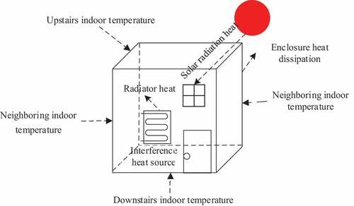
By describing the dynamic process of heat storage and the effect of each influencing factor, the indoor thermal equilibrium equations are established by mechanism modeling, which are shown in equations (1(1) $C_{wo}\frac{d{t}_{wo}}{d\tau }=h_{wo}{f}_{wo}\left(t_o-t_{wo}\right)+h_{woi}{f}_{wo}\left(t_{wi}-t_{wo}\right)+q_{sol}$(1) )~(6), and the characteristic coefficients representing the influencing factors of indoor temperature are obtained by solving the equations based on the state-space technique. The indoor temperature is predicted according to the influencing factors at the subsequent time.

(1) $C_{wo}\frac{d{t}_{wo}}{d\tau }=h_{wo}{f}_{wo}\left(t_o-t_{wo}\right)+h_{woi}{f}_{wo}\left(t_{wi}-t_{wo}\right)+q_{sol}$(1)

(2) $C_{wi}\frac{d{t}_{wi}}{d\tau }=h_{wi}{f}_{wi}\left(t_z-t_{wi}\right)+h_{woi}{f}_{wi}\left(t_{wo}-t_{wi}\right)+{\sum }_j{h}_{wj}\left(t_j-t_{wi}\right)$(2)

(3) $C_g\frac{d{t}_g}{d\tau }=h_g{f}_g\left(t_z-t_g\right)+q_{gf}$(3)

(4) $C_l\frac{d{t}_l}{d\tau }=h_{lo}{f}_l\left(t_o-t_l\right)+h_{li}{f}_l\left(t_z-t_l\right)+q_s$(4)

(5) $C_z\frac{d{t}_z}{d\tau }=\hspace{0.17em}\sum _i{h}_{wi}{f}_{wi}\left(t_{wi}-t_z\right)+\hspace{0.17em}\sum _l{h}_{li}{f}_l\left(t_l-t_z\right)+h_g{f}_g\left(t_g-t_z\right)+c_o\rho G_o\left(t_{out}-t_z\right)+q_{rad}+q_{fs}$(5)

(6) $C_z\frac{d{t}_z}{d\tau }=\hspace{0.17em}\sum _i{h}_{wi}{f}_{wi}\left(t_{wi}-t_z\right)+\hspace{0.17em}\sum _l{h}_{li}{f}_l\left(t_l-t_z\right)+h_g{f}_g\left(t_g-t_z\right)+c_o\rho G_o\left(t_{out}-t_z\right)+q_{rad}+q_{fs}$(6)

The matrix form of the total thermal dynamic equation of the building can be obtained by combining equations (1(1) $C_{wo}\frac{d{t}_{wo}}{d\tau }=h_{wo}{f}_{wo}\left(t_o-t_{wo}\right)+h_{woi}{f}_{wo}\left(t_{wi}-t_{wo}\right)+q_{sol}$(1) ) ~ (6) as shown in equation (7)(7) $\mathrm{C}\dot{T}=AT+BU$(7) .

(7) $\mathrm{C}\dot{T}=AT+BU$(7)

The characteristic coefficients${\lambda }_i$,${\phi }_{i,k}$ can be obtained by solving equations (5)(5) $C_z\frac{d{t}_z}{d\tau }=\hspace{0.17em}\sum _i{h}_{wi}{f}_{wi}\left(t_{wi}-t_z\right)+\hspace{0.17em}\sum _l{h}_{li}{f}_l\left(t_l-t_z\right)+h_g{f}_g\left(t_g-t_z\right)+c_o\rho G_o\left(t_{out}-t_z\right)+q_{rad}+q_{fs}$(5) and (6(6) $C_z\frac{d{t}_z}{d\tau }=\hspace{0.17em}\sum _i{h}_{wi}{f}_{wi}\left(t_{wi}-t_z\right)+\hspace{0.17em}\sum _l{h}_{li}{f}_l\left(t_l-t_z\right)+h_g{f}_g\left(t_g-t_z\right)+c_o\rho G_o\left(t_{out}-t_z\right)+q_{rad}+q_{fs}$(6) ). According to${\lambda }_i$, ${\phi }_{i,k}$and equation (7)(7) $\mathrm{C}\dot{T}=AT+BU$(7) , the dynamic model of the indoor temperature can be obtained as follows.

(8) $t_z(\tau )=t_{bz}(\tau )+{\sum }^{{\phi }_{o,0}}{t}_o(\tau )+{\phi }_{r,a}{K}_{ra}\frac{K_v\sqrt{\mathrm{\Delta }p}{R}^{x-1}({\bar{t}}_s-{\bar{t}}_r)}{f_{rad}}+{\phi }_{out}{t}_{out}(\tau )$(8)

where$t_{bz}\left(\tau \right)=\hspace{0.17em}\sum _i{e}^{{\lambda }_i\mathrm{\Delta }\tau }{t}_{zi}\left(\tau -\mathrm{\Delta }\tau \right)+\hspace{0.17em}\sum _k\left({\phi }_{k,1}{u}_k\left(\tau -\mathrm{\Delta }\tau \right)\text{break}+{\phi }_{k,0}{u}_k\left(\tau \right)\right)+\hspace{0.17em}\sum _o{\phi }_{o,0}{t}_o\left(\tau -\mathrm{\Delta }\tau \right)$indicates the indoor natural temperature without heating.

3.2. Verification of the indoor temperature predictive control model

According to the enclosure materials and outdoor climate conditions, the physical parameters of the building are shown in Table 2.

Table 2. Physical parameters of building.

$C_{wo}=6.05\times {10}^{6}J{/}^{\circ }C$	$h_{wo}=h_{wi}=1.45W/\left(m^2{\cdot }^{\circ }C\right)$	North window$f_l=5.4m^2$
$C_{wi}=5.2\times {10}^{7}J{/}^{\circ }C$	$h_{woi}=0.2W/\left(m^2{\cdot }^{\circ }C\right)$	$h_{l1}=h_{l2}=4.3W/\left(m^2{\cdot }^{\circ }C\right)$
South wall$f_{wo}=f_{wi}=27m^2$	$h_{wj}=0.2W/\left(m^2{\cdot }^{\circ }C\right)$	$C_g=6\times {10}^{6}J/{\hspace{0.17em}}_{\hspace{0.17em}}^{\circ }C$
North wall$f_{wo}=f_{wi}=30.6m^2$	$C_l=5\times {10}^{6}J{/}^{\circ }C$	$h_g=10W/\left(m^2{\cdot }^{\circ }C\right)$
East and west wall$f_{wo}=f_{wi}=36m^2$	South window$f_l=9m^2$	$f_g=25m^2$
$C_z=1.09\times {10}^{5}J{/}^{\circ }C$	$c_o=1\times {10}^{5}J/\left(kg{\cdot }^{\circ }C\right)$	$C_{rad}=2.94\times {10}^{4}J{/}^{\circ }C$
$\rho =1.26\mathrm{k}\mathrm{g}/m^3$	$f_{rad}=33.33m^2$	$K_v=6.3m^3/h$
$\overline{t_s}={60}^{\circ }C$	$\overline{t_r}={41.5}^{\circ }C$	$K_{rad}=2.84W/\left(m^2{\cdot }^{\circ }C\right)$

The calculation formula of indoor air temperature can be obtained by substituting them into formula (8).

(9) $\begin{array}{c}{t}_z\left(\tau +1\right)=t_{bz}\left(\tau \right)+0.08t_{o1}\left(\tau +1\right)+0.08t_{o2}\left(\tau +1\right)\text{break}+0.087t_{o3}\left(\tau +1\right)+0.094t_{o4}\left(\tau +1\right)\\ \hspace{0.17em}+6.96\times {30}^{x-1}+\text{break}0.0002\left(t_{out}\left(\tau +1\right)-t_z\left(\tau +1\right)\right)\end{array}$(9)

where$t_{o1},t_{o,2},t_{o,3},t_{o,4}$is the indoor temperature of four adjacent rooms of the building.

In the verification of the indoor temperature prediction model, the radiator valve opening degree and indoor temperature are collected by the BEMS; the outdoor wind speed is obtained by the local, small meteorological station; the solar radiation heat adopts the weather forecast data; and the heat gain coefficient of the window is 0.626 ⁽Ismail 2003⁾. During the experiment, the valve opening control signal is discretized into$U_k=\left\{0,0.1,0.2\dots 1\right\}$, and the sampling step is one hour. The indoor temperature sampling time is from 20 December 2017 to 26 December 2017, and 143 sampling points are taken every hour. The valve opening degree in the heating period is shown in Figure 2(a), and the comparison between the measured value of the indoor temperature and the predicted value of the model prediction is shown in Figure 2(b).

Figure 2. Validation of indoor temperature prediction model.

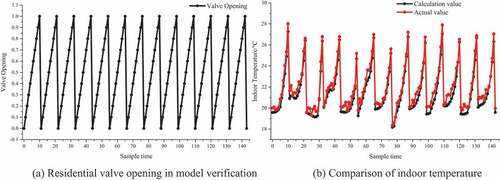
The root mean square error (RMSE) of the measured value and the predicted value of the indoor temperature control model is 0.02 °C, and the correlation coefficient R² is 0.884, which indicates that the indoor temperature control model can track the indoor temperature well.

3.3. Parallel pump model of the heat exchange station

In the high-rise residential building, the heat exchange station is divided into two parts: low area and high area. Low area heating is mainly responsible for the heating demand of floors 1–7, whereas high area heating is responsible for the heating demand of floor 8 and above. In the heat exchange station, three ISW40-160 (I) pumps are connected in parallel in the low area heating and three ISW80-200 pumps in the high area. The parameters of the water pump are shown in Table 3. The performance curve is shown in Figure 3. The ISW80-160A and ISW80-200 models are shown in equations (10(10) $H=35.7-0.019Q+3.32\times {10}^{-2}{Q}^2-3.27\times {10}^{-3}{Q}^3$(10) )~(13).

(10) $H=35.7-0.019Q+3.32\times {10}^{-2}{Q}^2-3.27\times {10}^{-3}{Q}^3$(10)

(11) $\eta =2.2+0.011Q-1.57\times {10}^{-2}{Q}^2+9.8133\text{break}\times {10}^{-4}\times Q^3$(11)

(12) $H=56.3-0.060Q+2.95\times {10}^{-3}\times Q^2-8.39\times {10}^{-5}{Q}^3$(12)

(13) $\eta =0.1+3.776\times Q-6.45\times {10}^{-2}{Q}^2+3.3392\times {10}^{-4}{Q}^3$(13)

Figure 3. Pump performance curve.

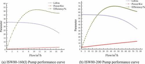
Table 3. Pump parameter.

Pump type	Rated Flow /$m^3/h$	Rated lift /$\mathrm{m}$	Rated efficiency /$\mathrm{\%}$	Shaft power /$f_{wo}=f_{wi}=30.6m^2$	Cavitation allowance /$\mathrm{m}$	Speed /$\mathrm{m}$
ISW40-160(I)	12.5	32	52	2.1	2.3	2950
ISW80-200	50	50	70	9.73	3	2950

where H is the pump head (m); Q is the flow of the pump ($m^3/h$); and$\eta$is the efficiency of the pump.

4. Decentralized optimization control methodology

4.1. Distributed control methodology

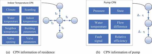
The basic concept of decentralized control is that local interactions between the components of a system establish order and coordination to achieve global goals without a central commanding influence, meaning that the overall system is no longer controlled by a single controller but by several independent local controllers incorporated into each component (Yi, Hong, and Liu 2015). Each residential entry valve is equipped with a distributed controller, which is used to control the valve opening to adjust the water intake of the radiator, thereby controlling the indoor temperature. The heat exchange station downstairs of the building is equipped with water pumps and heat exchangers, and each water pump and heat exchanger is also equipped with a distributed controller called the CPN(Computer Point Node) (Dai, Jiang, and Qi 2016). The physical structure of the building heating system shown in Figure 4, each CPN is connected to the heating system topology displayed in Figure 5, Each CPN only works with its neighbor to realize the control and optimization of the distributed heating system. The CPN information of the building space unit and water pump is shown in Figure 6 (a) and Figure 6(b).

Figure 4. Physical structure of heating building system.

Figure 5. Topology of heating building system.

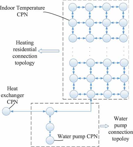
Figure 6. CPN information connection diagram.

4.2. Decentralized indoor temperature model prediction control

The goal of indoor temperature MPC controllers is to ensure that the temperature difference between the predicted temperature and the set temperature at the next moment is minimized. The objective function definition of the controller is shown in formula (14), and the design objective of the controller is shown in formula (15):

(14) $J\left(k\right)={∥t_z\left(k+N\right)-t_s∥}_W^2$(14)

(15) $\begin{array}{c}min\\ x\left(k\right)\end{array}{J}_k={∥t_a\left(k+N\right)-t_s∥}_W^2$(15)

where x(k) is the system control quantity (i.e., radiator valve opening).

According to research on human comfort (MH, Cao, and Ouyang et al. 2016), the setting range of indoor temperature is$18\le t_s\le {21}^{\circ }C$. The weight W is determined according to the temperature setting range, and the formula is shown in (16):

(16) $W=\{\begin{array}{cc}0& 18\le t_z\le 21\\ 1& t_z⟨18\mathrm{o}\mathrm{r}{t}_z⟩21\end{array}$(16)

The regulating range of valve opening is 0 ≤$x\left(k\right)$< 1. The coupling relationship between pipe networks is not considered temporarily during the experiment. The control steps in each sampling step based on the distributed indoor temperature model predictive control are shown in Figure 7. The indoor temperature of each residence is within the set value range after the distributed control, which ensures the thermal comfort of the building.

Figure 7. Flow chart of predictive control of distributed indoor temperature model.

4.3. Distributed control of water pumps in the heat exchange station

The optimization of the heat exchange station requires the optimal control of water pumps. All pumps are equipped with decentralized controllers to form CPNs. The optimization goal is to minimize the total energy consumption of pumps while ensuring that the water demand of users is met, which can be described as follows:

(17) $min\sum _{i=1}^m{\alpha }_i{p}_i$(17)

$s.t.\sum _{i=1}^m{\alpha }_i{x}_i=X$

${\alpha }_i\in \left\{0,1\right\}$

where ${\alpha }_i$is the opening status of each pump, and the value is 1 or 0, which corresponds to on and off, respectively; $m,p_i,x_i$and$X$are the number of parallel water pumps, energy consumption of each pump, flow rate of each pump, and total water supply required for building heating, respectively.

The efficiency-distribution variable of pump is a quadratic curve,as shown in Figure 6.The similarity law of the pump is shown in equation (18)(18) $\frac{Q(n)}{Q(n_0)}=\frac{n}{n_0},\frac{H(n)}{H(n_0)}={\left(\frac{n}{n_0}\right)}^2,\frac{\eta (n)}{\eta (n_0)}=1$(18)

(18) $\frac{Q(n)}{Q(n_0)}=\frac{n}{n_0},\frac{H(n)}{H(n_0)}={\left(\frac{n}{n_0}\right)}^2,\frac{\eta (n)}{\eta (n_0)}=1$(18)

When the pressure difference is the same between the two sides of the pump, equations (13)(13) $\eta =0.1+3.776\times Q-6.45\times {10}^{-2}{Q}^2+3.3392\times {10}^{-4}{Q}^3$(13) and (14(14) $J\left(k\right)={∥t_z\left(k+N\right)-t_s∥}_W^2$(14) ) can be used to show that the total efficiency is highest when each device operates at its highest efficiency. Therefore, the initial adjustment node is set to the highest efficiency point of the pump. During the iterative process, each pump is guaranteed to be at the highest efficiency point. The regulation mechanism of pump CPN is shown in Figure 8.

Figure 8. Principle of distributed optimization algorithm for parallel pumps.

After successive iterations, the error range of the difference between the water supply and demand of water pumps is reasonable. Controlling water pumps according to the operating point achieves the optimal control of the water pump system.

5. Results and discussion

This section presents the findings of distributed model predictive control and parallel pump distributed control.

5.1. Distributed indoor temperature model predictive control results

Because of the high installation cost of CPN, only 16 rooms on floors 12–15 of the No. 45 building of the teachers’ residential building in XAUAT were used to study the room temperature model predictive control. A CPN node was installed at the entrance of each room to control the room temperature. Data were collected on 16 January 2020, and the outdoor temperature is shown in Figure 9.

Figure 9. Outdoor temperature.

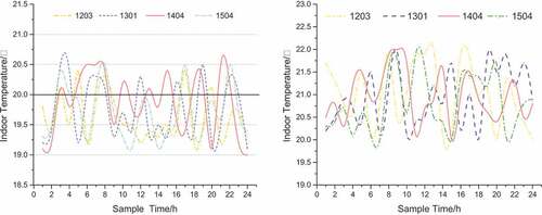
To verify the effectiveness of the MPC control, the temperature control valve was compared between rooms select 1203, 1301, 1404, and 1504, at a set temperature of 20°C(Figure 10). In thermostatic control, the temperature of each room fluctuates greatly. Because the temperature of adjacent rooms is not fully considered, the room temperature is higher than 20°C. Under DMPC control, the temperature of the four rooms is kept at the set temperature value, and the fluctuation does not exceed ±1°C.

Figure 10. Compersion between DMPC and Thermostatic control.

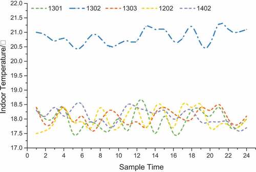
Figure 11 shows the results of the temperature experiment on the central room at the same temperature in adjacent rooms. The temperatures set for the 16 rooms are shown in Figure 11; the center room 1302 and four adjacent rooms (1301, 1303, 1202, and 1402) were studied, and these rooms are shown in the yellow box. The room temperature of 1302 is set to 21°C, and the temperature of the other four adjacent rooms is set to 18°C. The experimental results are shown in Figure 12. After optimization control, the temperature of the five rooms can be stabilized within the set value range, and the fluctuations are within ±0.5°C.

Figure 11. Indoor set temperature.

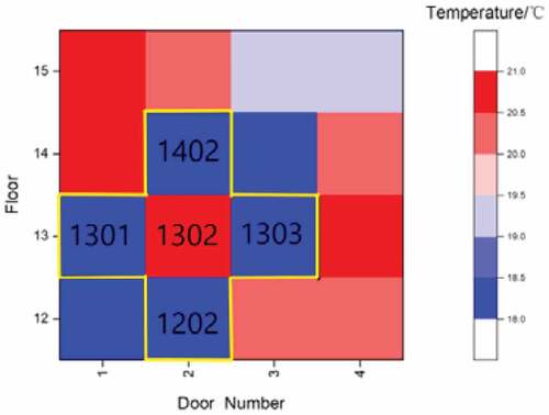
Figure 12. Indoor measured room temperature.

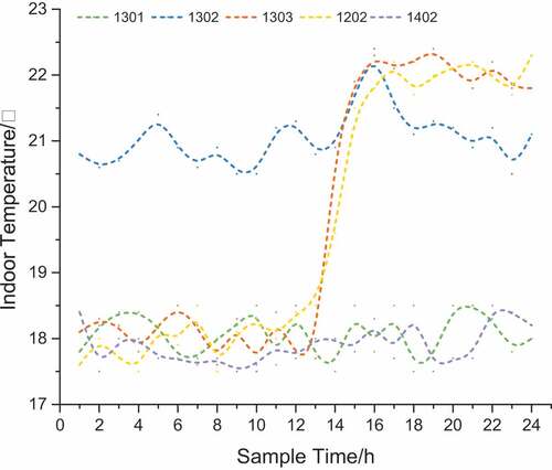
To study the effect of adjacent rooms on the temperature of the central room, the set temperature values of 1303 and 1202 were adjusted to 22°C at 13:00, and the set temperature values of the other rooms remained unchanged. The hot zone diagram is shown in Figure 13, and the experimental results are shown in Figure 14. When the temperature of 1303 and 1202 changes at 13:00, the indoor temperature of the two rooms reaches approximately 22°C after 2 h. Because of the lag in the heat transfer of the wall, the temperature of 1302 in the central room increased from 20.8°C to 22.4°C from 14:00 to 15:00 . However, the temperature set in 1302 did not change. After the temperature sensor detected the abnormal temperature, it controlled the valve in a timely manner, which caused the room temperature to decrease to 17°C and the set value to increase to 21°C. During the temperature change, the room temperature of 1301 and 1402 fluctuated little because of the timely response of the temperature control valve of 1302 and the hysteresis of the wall heat transfer process.

Figure 13. Indoor set temperature.

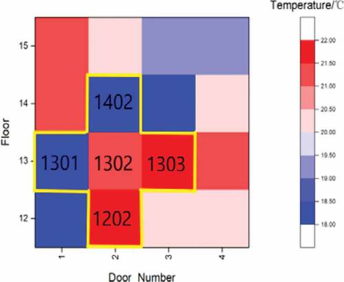
Figure 14. Indoor measured room temperature.

To verify the effect of adjacent rooms on the opening of the temperature control valve in the central room under the same outdoor conditions, the rooms 1401, 1501, 1502, 1203, 1204, and 1304 were studied. The room temperature setting is shown in the yellow box in Figure 15. Rooms 1501 and 1204 are both set to 20°C, 1401 and 1502 are both set to 17°C; and 1203 and 1304 are set to 22°C and 24°C, respectively. Figure 16 shows that the temperature of these 6 rooms is maintained near the set value, and the fluctuations do not exceed ±0.5°C, but the valve opening of 1501 is basically maintained at 0.6 in Figure 17. Because the temperature of rooms adjacent to 1204 is relatively high, the valve opening only needs to be kept at 0.4 to reach the set temperature. Therefore, the influence of adjacent rooms on the room temperature of the central room requires consideration when modeling the indoor thermal environment.

Figure 15. 1501, 1204 and their adjacent room temperature setting value.

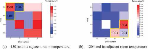
Figure 16. 1501,1204 and their adjacent room measured temperature.

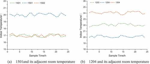
Figure 17. 1501,1204 and their adjacent room Valve opening value.

5.2. Distributed control results for the water pumps

After determining the heating water consumption of the residential building, the distributed control optimization of pumps in the heat exchange station was conducted using the high area pump ISW 80–200 as an example. The three water pump CPNs in the high area are connected in parallel to form an integral module. The water pump adopts constant pressure difference control and is set to 50 m. After the distributed control of the indoor temperature of the building on 16 January 2019, the water demand in the high area was 87 m³/h at 17:00, and the final regulated flow convergence threshold was kept within ± 1 m³ /h. The initial values of the flow and efficiency of the three pumps are shown in Table 4.

Table 4. Initial state of parallel circulating water pump.

Water pump number	No.1	No.2	No.3
Flow /m^3/h	29	29	29
Energy/%	61.19	61.19	61.19

During the regulation process, pump 3 is selected as the initial adjustment point; thus, the efficiency of pump 3 is adjusted to the maximum and the relative efficiency$\eta { }^{\mathrm{\prime }}=1$. After the calculation of the pump 3 CPN, $\mathrm{\Delta }=20.18m{\hspace{0.17em}}_{\hspace{0.17em}}^3/h$ is calculated at this time, the system supply flow rate is 20.18 m³/h more than the required flow rate. The pump 3 CPN then sends the$\mathrm{\Delta }$and $\eta { }^{\mathrm{\prime }}$ to the pump 2 CPN. After receiving the transmitted parameters, the pump 2 CPN calculates the $\mathrm{\Delta }$and$\eta { }^{\mathrm{\prime }}$ according to the same rule and passes the calculated result to the pump 1 CPN, which performs the same calculation and passes the result to the adjacent CPN. The iterative calculation is repeated until the regulation stops. When the deviation between the system supply flow and the required flow reaches 0.77 m³/h, the algorithm convergence condition is satisfied, and the calculation is stopped at this time. The water supply and efficiency of the three pumps at this time are shown in Table 5. The current operating frequency of each CPN is transmitted to the pump controller, and the pump is adjusted according to the final control signal.

Table 5. Optimized state of parallel circulating water pump.

Water pump number	No.1	No.2	No.3
Flow/m^3/h	44.01	0	43.76
Energy /%	71.47	0	71.40

The entire iterative adjustment process is shown in Figure 18(a). At the beginning of the next control cycle, the pump CPN receives the predicted heating water demand of the building. Based on the regulation results of the above control cycle, the control quantity of each pump in the new cycle is calculated according to the same iterative algorithm. The required heating water volume for the building high area is 107 m³/h at 18:00. The iterative process of the CPN of each pump based on the adjustment state at 17:00 is shown in Figure 18(b).

Figure 18. Iterative process of distributed algorithm for circulating water pump.

The pump 2 CPN initiates the start-up and adjusts according to the received relative efficiency at 18:00 because of the increase in water demand (Figure 18(b)). In the subsequent process, the CPN of each pump still operates according to the established iterative algorithm until the supply and demand error reaches a reasonable range; the calculation is then stopped, The parallel pump in the high region at 17:00 was taken as the analysis object of the optimization results. The flow efficiency comparison before and after the optimal control is shown in Figure 19.

Figure 19. Comparison before and after pump optimal control at 17:00.

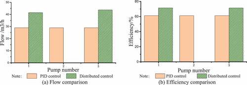
The efficiency of pump 1 is 71.47%, which is 16.8% higher compared with before the optimization; pump 2 is stopped after optimization; and the efficiency of pump 3 after optimization is 71.40%, which is 16.6% higher compared with before optimization (Figure 19). The efficiency of the entire parallel pump system increased by 16.74% compared with the efficiency before optimization.

The overall efficiency of the water pump system is significantly improved after the distributed control. Figure 20 shows the flow and efficiency of each pump in the heat exchange station before and after optimization.

Figure 20. Pumps state before and after distributed optimization.

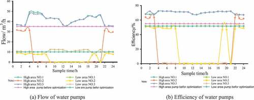
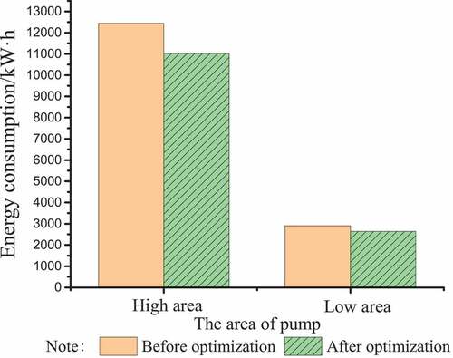
In Figure 20, each water pump in the high and low areas undertakes the same workload before optimization, as shown by the pink triangular lines and green diamond lines in the figure. The overall efficiency of the water pump is low. After optimization, each circulating water pump can independently adjust the operation frequency according to different total flow requirements, and the overall efficiency is 16.74% higher compared with before optimization. Figure 21 shows the comparison of energy consumption of pumps in high and low areas before and after optimization in a day. The energy consumption of pumps in high areas after optimization is reduced by 11.36% and in low areas by 9.04%; the total energy consumption is reduced by 14.28%.

Figure 21. Comparison of energy consumption of pump before and after optimization.

6. Conclusion

In this paper, the influencing factors of temperature between adjacent rooms are considered, and after the distributed model predictive control of residential indoor temperature, the temperature control accuracy of each room is improved, and the error is kept within 0.7 °C. At the same time, after the distributed control of circulating water pump in heat exchange station, the individual efficiency of water pump is increased by more than 16%, the overall efficiency is increased by 16.74%, and the energy consumption is reduced by 14.28%.

Future work will focus on the dynamic cost function. According to the form of stepped electricity prices, comprehensive consideration of thermal comfort and energy-saving effects, according to the peak and valley electricity prices to adjust the opening of the door radiator valve and the frequency of parallel water pumps,establish a multi-objective function, and improve the efficiency of central heating economy.

Disclosure statement

No potential conflict of interest was reported by the author(s).

Additional information

Funding

This work was supported by the Key Technologies and Demonstration of Green Building Energy Consumption Management Analysis Platform Based on Big Data [2017ZDL-SF-16-5].

Notes on contributors

Zhou Meng

Zhou Meng,  Ph.D candidate, research direction is energy management optimization, intelligent building prediction and control.

YU Junqi

Yu Junqi, Ph.D. Professor, current research direction is building intelligence and energy-saving control technology, building energy consumption monitoring and information management system, intelligent automation system and application.

Zhao Anjun

Zhao Anjun, Ph.D.  Associate professor. Currently accommodated in the direction of building networking and big data analysis, intelligent building HVAC control and optimization, large-scale public building energy consumption detection and energy saving analysis, intelligent building detection technology.

References

- Afroz, Z., G. M. Shafiullah, and T. Urmee. 2017. “Prediction of Indoor Temperature in an Institutional Building[J].” Energy Procedia 142: 1860–1866. doi:10.1016/j.egypro.2017.12.576.
- Ali, M., A. Alahäivälä, F. Malik, and M. Humayun. 2015. “A Market-oriented Hierarchical Framework for Residential Demand Response.” International Journal of Electrical Power & Energy Systems 69: 257–263. doi:10.1016/j.ijepes.2015.01.020.
- Barán, B., C. von Lücken, and A. Sotelo. 2005. “Multi-objective Pump Scheduling Optimisation Using Evolutionary strategies[J].” Advances in Engineering Software 36 (1): 39–47. doi:10.1016/j.advengsoft.2004.03.012.
- da Costa Bortoni, E., R. A. de Almeida, and A. N. C. Viana. 2008. “Optimization of Parallelvariable-speed-driven Centrifugal Pumps operation[J].” Energy Efficiency 1 (3): 167–173. doi:10.1007/s12053-008-9010-1.
- Dahlblom, M., B. Nordquist, and J. Lars. 2018. “Evaluation of a Feedback Control Method for Hydronic Heating Systems Based on Indoor Temperature measurements[J].” Energy and Buildings 166: 23–24. doi:10.1016/j.enbuild.2018.01.013.
- Dai, Y., Z. Jiang, and S. Qi. 2016. “A Decentralized Algorithm for Optimal Distribution in HVAC systems[J].” Building and Environment 95: 21–31. doi:10.1016/j.buildenv.2015.09.007.
- De Dear, R. J. 1998. “A Global Database of Thermal Comfort Field experiment[J].” ASHRAE Transactions 104 (1): 1141–1152.
- DEPAULA XAVIER, A. A., and R. Lamberts. 2000. “Indices of Thermalcomfort Developed from Field Survey in Brazil[J].” ASHRAE Trans 106 (Part1): 45–58.
- Embaye, M., R. K. A. L. Dadah, and S. Mahmoud. 2016. “Effect of Flow Pulsation on Energy Consumption of a Radiator in a Centrally Heated Building [J].” International Journal of Low-Carbon Technologies 11: 119–129.
- Embaye, M., A.-D. R K, and S. Mahmoud. 2016. “Numerical Evaluation of Indoor Thermal Comfort and Energy Saving by Operating the Heating Panel Radiator at Different Flow strategies[J].” Energy and Buildings 121: 298–308. doi:10.1016/j.enbuild.2015.12.042.
- Gao, B., L. Zhang, and T. Yanfa. 2017. “Analysis on Energy Saving Measures of Heat Exchange Station in Central Heating system[J].” Procedia Engineering, no. 205: 581–587. doi:10.1016/j.proeng.2017.10.422.
- Gao, S. 2019. “Design and Analysis of Energy-saving and Thermal Insulation Technology for New Green Building Wall Materials [J].” Journal of Lanzhou Institute of Technology 26 (3): 29–33.
- GB50096-2011 “Residential design specification [S]”. 2012.
- Gong, E., N. Wang, and Y. Shijun. 2019. “Optimal Operation of Novel Hybrid District Heating System Driven by Central and Distributed Variable Speed pumps[J].” Energy Conversion and Management 196: 211–226. doi:10.1016/j.enconman.2019.06.004.
- Gu, J., J. Wang, Q. Chengying, and B. Sundén. 2019. “Analysis of a Hybrid Control Scheme in the District Heating System with Distributed Variable Speed pumps[J].” Sustainable Cities and Society 48: 101591. doi:10.1016/j.scs.2019.101591.
- Hedegaard, R. E., T. Pedersen, and K. MichaelDahl. 2018. “Towards Practical Model Predictive Control of Residential Space Heating: Eliminating the Need for Weather Measurements [J].” Energy and Buildings 170: 206–216. doi:10.1016/j.enbuild.2018.04.014.
- Ismail, K. 2003. “Modeling and Simulation of a Simple Glass Window.” Solar Energy Materials and Solar Cells 80 (3): 355–374. doi:10.1016/j.solmat.2003.08.010.
- Junqi, Y., L. Qite, and Z. Anjun. 2021. “A Distributed Optimization Algorithm for the Dynamic Hydraulic Balance of Chilled Water Pipe Network in Air-conditioning system[J].” Energy 223(120059): 1-13. doi:10.1016/j.energy.2021.120059
- Kim, M. S., Y. Kim, and C. Kwang-Seop. 2010. “Improvement of Intermittent Central Heating System of University building[J].” Energy and Buildings 42 (1): 83–89. doi:10.1016/j.enbuild.2009.07.014.
- Kolokotsa, D., A. Pouliezos, and G. Stavrakakis. 2009. “Predictive Control Techniques for Energy and Indoor Environmental Quality Management in Buildings [J].” Building and Environment 44 (9): 1850–1863. doi:10.1016/j.buildenv.2008.12.007.
- Lauenburg, P., and J. Wollerstrand. 2014. “Adaptive Control of Radiator Systems for a Lowest Possible District Heating Return temperature[J].” Energy and Buildings 72: 132–140. doi:10.1016/j.enbuild.2013.12.011.
- Luo, M., Cao, B., Ouyang, Q., Zhu, Y. 2016. “Indoor Human Thermal Adaptation:dynamic Process and Weighting facors[J].” Indoor Air 27 (2): 273–281.
- Ma, J., J. Qin, T. Salsbury, and P. Xu. 2012. “Demand Reduction in Building Energy Systems Based on Economic Model Predictive control[J].” Chem. Eng 67 (1): 92–100. doi:10.1016/j.ces.2011.07.052.
- Miezis, M., D. Jaunzems, and N. Stancioff. 2017. “Predictive Control of a Building Heating System[J].” Energy Procedia 113: 501–508. doi:10.1016/j.egypro.2017.04.051.
- Nielsen, H. A., and H. Madsen. 2006. “Modeling the Heat Consumption in District Heating System Using a Grey-box approach[J].” Energy and Buildings 38 (1): 63–71. doi:10.1016/j.enbuild.2005.05.002.
- Nora, C., L. Andrea De, and G. Agostino. 2018. “A Model-in-the-Loop Application of A Predictive Controller to A District Heating system[J].” Energy Procedia, 148(2018):352–359. doi:10.1016/j.egypro.2018.08.088.
- Pedersen, T. H., R. E. Hedegaard, and S. Petersen. 2017. “Space Heating Demand Response Potential of Retrofitted Residential Apartment blocks[J].” Energy and Buildings 141: 158–166. doi:10.1016/j.enbuild.2017.02.035.
- Prívara, S., J. Široký, L. Ferkl, and J. Cigler. 2011. “Model Predictive Control of a Building Heating System: The First experience[J].” Energy and Buildings 43 (2–3): 546–572. doi:10.1016/j.enbuild.2010.10.022.
- Sun, F., B. Hao, and L. Fu. 2021. “New Medium-low Temperature Hydrothermal Geothermal District Heating System Based on Distributed Electric Compression Heat Pumps and a Centralized Absorption Heat transformer[J].” Energy 232. doi:10.1016/j.energy.2021.120974.
- Tahersima, F. 2013. “Jakob Stoustrup, Henrik Rasmussen. An Analytical Solution for Stability-performance Dilemma of Hydronic radiators[J].” Energy and Buildings 64 (5): 439–446. doi:10.1016/j.enbuild.2013.05.023.
- Thermal adaptation and thermal environment in university classrooms and offices in Harbin[J]. 2014. “Zhaojun Wang,Aixue Li,Jing Ren,Yanan He.” Energy and Buildings 77: 192–196.
- Viholainen, J., Tamminen, J., Ahonen, T. et al. 2013. “Energy-efficient Control Strategy for Variable Speed-driven Parallel Pumping systems[J].” Energy Efficiency 6 (3): 495–509. doi:10.1007/s12053-012-9188-0.
- Wang, J., Z. ZJ, and Y. Jing. 2011. “Influence Analysis of Building Types and Climate Zones on Energetic, Economic and Environmental Performance of BCHP systems[J].” Applied Energy 88 (9): 3097–3112. doi:10.1016/j.apenergy.2011.03.016.
- Wang, Y., S. You, X. Zheng, and Z. Huan. 2017. “Accurate Model Reduction and Control of Radiator for Performance Enhancement of Room Heating system[J].” Energy and Buildings 138: 415–431. doi:10.1016/j.enbuild.2016.12.034.
- Wong, L. T., K. W. Mui, and T. W. Tsang. 2018. “An Open Acceptance Model for Indoor Environmental Quality (IEQ)[J].” Building and Environment 142: 371–378. doi:10.1016/j.buildenv.2018.06.031.
- Yi, P., Y. Hong, and F. Liu. 2015. “Distribute Gradient Algorithm for Constrained Optimization with Application to Load Sharing in Power systems.[J].” Systems & Control Letters 83: 45–52. doi:10.1016/j.sysconle.2015.06.006.
- Yu, T., X. Wang, J. Ji, and Z. Shumin. 2017. “Energy Efficiency of Distributed Energy System Based on Central Heating network[J].” Procedia Engineering 205 (205): 2171–2175. doi:10.1016/j.proeng.2017.10.039.
- Zhang, L., O. Gudmundsson, J. E. Thorsen, 2016. “Method for Reducing Excess Heat Supply Experienced in Typical Chinese District Heating Systems by Achieving Hydraulic Balance and Improving Indoor Air Temperature Control at the Building level[J]”. Energy 107: 431–442. doi:10.1016/j.energy.2016.03.138