Describing the geometric difference of architectural forms in three primary shapes of circle, triangle and square

ABSTRACT

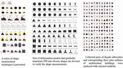
Defining architectural shapes and then clarifying their geometric differences has always been a demanding task.. There appears to be relatively few research papers on the description of the definite geometric properties in architectural shapes. This research proposes methods for quantitatively describing an architectural shape as the degree to which they represent the three primary shapes of circles, triangles and squares. History has ensured that the shapes are regarded as primary ones, but any shape can also be viewed as one of them. A series of automated models that gradually deform the basic shapes into other forms have been developed to identify and verify the best methods for describing the architectural forms. The three architectural shape descriptors, referred to as “circularity”, “triangularity” and “squareness”, produce the second index of “shape deformity”, measuring the degree of how a shape is deformed from the primary shapes. This measurement makes it possible to investigate the degree to which a particular type of primary shape is dominant among those three primary shape descriptions. These shape description techniques were tested on 60 shapes consisting of the facades and floor plans of 30 well-known buildings.

Graphical Abstract

KEYWORDS:

• Primary shapes
• shape description
• geometric property

1. Introduction

Figure 1 shows two well-known buildings representing the art of freestyle modern architecture and their silhouette images. It is not difficult to see that the shape of the Guggenheim Museum Bilbao is much more heterogeneous and versatile than that of Ronchamp Chapel. The human ability to instantly grasp the difference in the shapes of the two buildings is the outcome of millions of years of evolution. It is, however, much more challenging to describe how they are different in their shapes, particularly considering architectural design features that have some irregularly protrusive forms with curved lines. Given the growing number of deformed shapes in architectural design nowadays, many research works on the representation and description of these shapes have been published not only with digital image sensing topics (Zang and Lu, 2004) but also environment psychology subjects (Greenfield 2005; Iigaya et al. 2021). A few published studies have reported on the measures of architectural shape description, mainly in dealing with visible space volume, referred to as “isovist shape analysis” (Batty 2001; Benedikt 1979; Stamps 2000).

Figure 1. Façade shapes of Ronchamp Chapel and Guggenheim Museum Bilbao

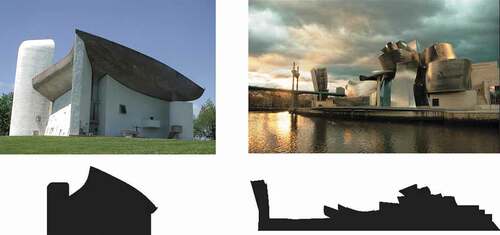
The main idea of the isovist shape analysis is how we perceive a volume of visible space or fields, and our movements in the fields depend on the geometric properties of the shape. Based on the properties obtained by measuring the shape’s distance, area, and perimeter, more sophisticated geometric measures were produced, such as compactness, complexity, eccentricity, and so on. This approach suggests well-defined mathematical formulae making it possible to quantify geometric properties. But they aren’t easy to be employed in the description of geometrical properties of architectural silhouettes and therefore to be used to quantify their differences given purely architectural form in two dimensions. It could be explained in the nature of the isovist shape, or the form of isovist fields, having its form formulated not by the geometric one only but by “the interaction of geometry and movement” (Batty 2001, 123). If the geometric architectural shapes are clearly described and clarify the difference between the shapes based on the geometry in design, it is possible to understand the design ideas deep inside a building form.

This study approaches the quantification of architectural shape on the premise that the three primary forms of circle, triangle and square can be criteria of the composition of an abstract unit shape to describe an architectural shape. This premise is supported by the neurological tendency to search for the simplest figures in objects (Arnheim, 1974; Pasupathy, El-Shamayleh, and Popovkina 2019; Rebe, Schwarz, and Winkielman 2004; Witkin and Tenenbaum 1983). These legacies of the fundamental notion of vision and perception enable us to hypothesize that a shape can be described through the essential factors of the three primary shapes, the simplest and the most basic shapes to standardize.

This study uses two-dimensional shapes of building facades and floor plans to explore the shape properties of architectural buildings. The facade is formed by gazing at a building in a specific location, providing the aesthetic value of the atmosphere and the intuitive interpretation of the building’s functionality. The floor plan accommodates the functional arrangement of the spatial structure and the visual perception inside a building. Based on the two types of figures, we propose the methods for evaluating both types of architectural form as the degree to which the morphological features of these three primary shapes are embedded. Exploring the shape properties of circularity (C), equilateral triangularity (T) and squareness (S) based on the three shapes will be the central theme of this study. It will also be introduced that the functions derived from these measurements can also quantitatively describe shape features globally, such as the deformation ratio (Deformity) and the most dominant shape with its ratio (Dominance).

The acronym “TPS” will refer to “the three primary shapes of circle, equilateral triangle and square”. For convenience, triangularity will indicate the shape properties of an equilateral triangle unless otherwise specified. This research begins with the organization of the theoretical dimensions and then looks at the background factors that support the legitimacy of TPS measurements. It then examines the techniques and concepts of the algorithms for the shape measurements. Based on the correlation with the gradual deformation model, a series of shape measurement techniques will be presented, evaluated, and verified. Finally, the TPS measurement results of a case study for 60 different shapes of well-known buildings will be illustrated to verify the methodology.

2. Description of architectural shape

2.1. Elements of visual perception

The visual delight of architecture begins with how we perceive it (Brachmann and Redies 2017), where perception starts by grasping dominant structural features (Arnheim, 1974) and their elements. This study focuses on outline shapes of architectural forms both on the facades and the floor plans, among many elements of architectural shapes. It is indisputable that human perception of shape depends on the degree of visual contrast in the contour, separating a figure from its background. The contour, also known as an outline, edge, or silhouette, is formed with sudden changes in some gradient such as colour, shadow, parallel lines seen in perspective, or texture when an object is projected through a lens onto the surface retina.

Neurophysiological studies have found that the area in the cortex of the primate’s brain is responsible for shape recognition and demonstrated for many decades that boundary contours allow the most substantial recognition of objects (Kim, Bair, and Pasupathy 2019; Pasupathy, El-Shamayleh, and Popovkina 2019). Witkin and Tenenbaum (1983) have shown that the boundary contour readily overrides perceptual interpretation of the luminance gradient of the three-dimensional objects. Biederman and Ju (1988) proved that, in reality, a simplified outline drawing was recognized as quickly and accurately as a photographic image of the same object described in full detail with its original colour and textures. Rebe, Schwarz, and Winkielman (2004) confirmed that pictures with matched contours were recognized faster in psychology. These works justify the use of silhouette images of the architectural shape for the subject of this study.

Since the outline depends on its orientation, we assumed that the polygon extracted from the building’s silhouette for shape measurement is in the front view, corresponding to the ground towards the x-axis. In architecture, Stamps (2000) examined geometric variables such as complexity, compactness, symmetry, simplicity, and elongation to interpret characteristics of architectural shape in discrete and descriptive ways. A comprehensive review of contour-based shape descriptors such as area, perimeter, compactness, eccentricity, and some moment functions from Zhang and Lu (2004) provides ways of inspecting the geometric properties mathematically. This study will suggest a series of methods to measure shapes with geometric regularity and simplicity using TPS.

2.2. Three primary shapes in architecture

There has been widespread agreement that the term “form” is identical regardless of orientation, whereas “shape” differs with every transformation (Bingham 1914; Fellow 1968; Gellermann 1933). In this regard, the shape is appropriate for the façade while the form is appropriate for the floor plan, but these terms will be used interchangeably for convenience.

The quest for the utilization of the TPS in making symbols or forms dates back to ancient times. Yantra, where TPS were superimposed for meditation in ancient India (11,000–10,000 BP), and the alchemists’ “Squared Circle”, which was used to describe the interaction of three vital elements in the universal psyche (Holmyard 1957; Jung 1968, 1964) are some of the examples. Oikonomou (2021) showed that the geometrical constructions based on circles, triangles and squares had been used in design and construction throughout history. TPS has been the symbol of divinity, femininity, masculinity, and their dynamics in their derived shapes. They could be expanded or rotated to create distinct, regular, and easily recognizable volumetric shapes or solids. It is easy to find the forms in everyday life, such as traffic signs and company logos.

There have been biological studies showing that specific geometric shapes are fundamental to perception. For example, a shape contributes to human satisfaction and is regarded as good when simple and unified. Kellogg (1970) found that specific primary forms such as a diagonal cross, circle, triangle and square appear in children’s scribbling. Piaget and Inhelder (1956) showed that children’s shape development progresses from the square vs circle, and then angle and dimension discrimination (Rosin 2003). Nineteenth-century art movements expressed the intrinsic structural properties of objects in primitive geometric forms by reducing objects to their most simplified forms through omitting details. The fundamental idea of perceiving an architectural shape is originated from the Gestalt theory that sought visual satisfaction and pleasure. Gestalt psychology emphasized that some primary forms of circle, triangle, and rectangle are “good” because they are simpler or easier to recognize or describe. Besides other perception theories, this theory has influenced architects to understand the aesthetic perception of the environment (Yılmaz, Özgüner, and Mumcu 2018).

In twentieth-century Germany, Bauhaus’s enthusiastic use of the primary forms in design principles was inspired by the Gestalt theory that sought an accurate way of recognizing form (Lupton and Miller 1991; Smock 2004). Pursuing a design prototype has encountered empirical studies in various experiments: For instance, Zusne (1970) concluded that certain forms were preferred over others in the process of visual perception; Arnheim (1974) found that perception started by grasping outstanding structural features; Helmholtz, 1924figured out that the more easily we perceived the order we characteriz the object observes, the simpler and the more perfect would they appear..

These pioneering principles led us to the reasonable foundation for describing architectural geometry with TPS’s simplest and most fundamental shapes. They are still used in many disciplines related to vision and are found in many textbooks (Gordon 2004; Metzger 2006). Meanwhile, it has been widely accepted that “the simpler the plan shape, the lower will be its unit cost” as a general rule (Seeley 1983; Wing 1999). While some evidence supported the impact of building facades (Stamps 1999) and height (Lindal and Hartig 2013) on the impression of buildings or their environments, Steadman (2014, 2006) showed that the form of the architectural plan was primarily classified as TPS and suggested that each form offered distinctive characteristics.

By definition, a circle is the locus of all points equidistant from a central point. It encloses the most space inside the shortest perimeter of all shapes and is considered perfect and compact by definition. Schneider (1995) traced ancient philosophers who believed that the circle represented the number one. Ching (2007) appreciated the circle in architecture as a centralized, introverted form that is usually stable and self-centring in its environment. Vartanian et al. (2013) showed that curvilinear contour activated the brain region more strongly responsive to objects’ reward properties and emotional salience than rectangular shapes through an fMRI experiment in neuroscience.

Regarding the social and functional interpretation of the three primary shapes, the square is defined as a convex quadrilateral with sides of equal length positioned at right angles to each other. It is stable when standing on one of its sides and felt in general with equality, reliability, fairness, firmness, solidity and a balanced state of equilibrium, as Schneider (1995) stated. Steadman (2014) explained that Bemis and Burchard’s (1933-36) earlier finding of the predominance (83%) of rectangular housing design was due to dimensioning flexibility. This rectangular predominance in the house plan is consistent with Krüger’s (1979)subsequent finding, where the rectangular design dominates at 98%. The efficiency of the horizontal and vertical loading of building components is one of their most critical elements. He deduced that the significance of the geometric arrangement of triangles and circles succeeded the importance of the rectangle for the same reason.

An equilateral triangle is a three-sided plane with all sides equal and equiangular. A building facade in a triangular shape with the vertex pointing upwards converges the most at the apex, facilitating stability and reliability in building design. Heavy base and the pinnacle on the top in many A-framed residential homes enable handling weight because of how the energy is distributed throughout the triangle; the symmetry in the equilateral triangle and the isosceles triangle aids in distributing weight. Trusses exist as bearing structures because of the inherent triangles provided by struts and other bracing elements (Lenartowicz 2014). The Pyramid in Giza, composed of four equilateral triangular faces, has stood for over 4,000 years. The equilateral triangle encloses the smallest area in the most extended perimeter and is a basic unit representing the three-dimensional surface. On the other hand, it can be seen that the triangular-shaped floor plan is unpractical from a functional point of view, as walls converging at an acute angle of 60° contain narrow leftover margins.

2.3. Evaluation of the shapes

Measures to grasp the topological properties of the geometric shapes emerged from diverse backgrounds. Birkhoff (1933) first classified the measures of various forms into complexity, vertical symmetry, equilibrium, rotation symmetry, and horizontal and vertical relationships. This has been widely accepted, modified and improved (Berlyne, 1971; Eysenck, 1942). The seventy-five years of history following his research of the computational measurement of geometric properties were reported by Greenfield (2005). Since then, Bar and Neta (2006) showed that curvilinear contour activated the brain region strongly responsive to objects’ reward properties and emotional salience. Redies(2007)presented the general aspect of visual information processing implemented by our visual brain. Meanwhile, Iigaya et al. (2021) asserted that human preferences for art could be explained as a systematic integration over the underlying visual features of an image.

Further research on the simple topological properties of the geometrical shapes emerged to explain the association between forms of visible space and perceptual activities. Zusne (1965) extracted that compactness, symmetry, and elongation could be computed with moments of area, which emerged as the predictors of some perceptual tasks. Brown and Owen (1967) categorized random shapes to be measured and developed variables based on the geometric properties, later extracted into three characteristics of compactness, jaggedness, and skewness by Zusne (1970).

Stamps (2000), who viewed the complexity as crucial in architecture and its built environment, concluded that the most significant factor determining shape complexity in building silhouettes is the number of vertices. Similarly, Franz and Wiener (2008) categorized the measurements, derived from the form of isovists and visibility graph theory introduced by Benedikt (1979)and Hillier and Hanson (1984), respectively, into four essential spatial qualities. These measurements included features such as jaggedness, revelation, roundness, clustering coefficient, symmetry and redundancy. As their research suggested the examples of expressing movement involved geometric forms, it has become intriguing to map explicitly selected vocabularies, describing the human perception of the geometric properties in architectural design, onto mathematical descriptors of the building forms. While this approach in measuring the shapes known as “isovist geometry” (Conroy 2000) involves the idea of embedding spatial experience in a visible area that is subdivided by a grid, what this study proposes is the way how to describe the pure geometric difference of building forms with architectural design terms, such as the primary architectural shapes.

3. Measuring Methods of Architectural Shapes with TPS

This chapter proposes the shape measurement methods of circularity, equilateral triangularity, and squareness (C, T, and S) based on the nature of the TPS. One of the letters of C, T and S, followed by a series of numbers, designates distinct primary shapes and quantification methods.

3.1. Common attributes of TPS for the shape measurements

This section explores the conventional attributes applicable to estimating circularity, triangularity, and squareness and covers the key concepts shared throughout the measurements. The mathematical expressions of all the shape measurements considered in the study are presented in Tables 1. Initial insight was inspired by an extensive review of the shape representation techniques conducted by Zhang and Lu (2004) and employed in this study’s architectural shapes. The architectural image captured by a flat-screen or the retina of an eye furnishes an intuitive model of a function with two variables (x, y) in the Euclidean plane as a polygon represented with a set of vertices v_i. Hence, here we will view this flat architectural image as polygon P and use these geometric properties to provide quantitative measurement methods.

Table 1. Measurements of circularity

Label	Expression
C1	C1 = $\frac{4\pi A}{L^2}$, where A = Area of the object polygon, L = Perimeter of the object polygon
C2	C2 = C1CH·C, where C = A/ACH, CH = Convex Hull of the polygon, C = Convexity
C3	C3 = 1 – (σrR/RRCA) ri = radial distance from centre to each vertex, RRCA = radius of RCA
C4	C4 = 1 – Δ(PRCA, Po), Δ(PRCA, Po) = (${\mathrm{P}}_{\mathrm{R}\mathrm{C}\mathrm{A}}\oplus {\mathrm{P}}_{\mathrm{o}}$)/(PRCA ∪ Po)
C5	C5 = 1 – $({\sigma }_{\hat{r}R}/R_{RCR}),{\hat{r}}_i$= radial distance from the center to evenly distributed points on the boundary line. RRCR: radius of the RCR
C6	C6 = 1- Δ(PRCR, Po), Δ(PRCR, Po) = (${\mathrm{P}}_{\mathrm{R}\mathrm{C}\mathrm{R}}\oplus {\mathrm{P}}_{\mathrm{o}}$)/(PRCR ∪ Po)
C7	C7 = RMIC/RMCC
C8	C8 = AMIC/A
C9	C9 = AMIC/AMCC
C10	C10 = A/AMCC
C11	C11 = $1-\frac{{\sigma }_{\varphi \pi }}{\pi }$, ϕ = mod(θ, π)
C12	$\psi \cdot r$, for |ψ| < 1.0, where ψ = θ/π, r = segment length(|ψ| <1.0)/total perimeter
C13	sin(θ/2), for |ψ| < 1.0, r = segment length(|ψ| <1.0)/total perimeter

Table 2

Table 2. Measurements of triangularity

Label	Expression
T1	T1 = $\frac{12A\sqrt{3}}{L^2}$ A = Area of the P, L= Perimeter of the object polygon, P = object polygon of the building shape.
T2	T2 = ART/A, ART = Area of RT derived from P, RT = (p1, p2, p3), where $p_1=\left(\left(x\right),\left(y\right)\right),p_2=\left(\left(x\right),\left(y\right)\right),p_3=\left(x\left(\left(y\right)\right),max\left(y\right)\right)$
T3	T3 = T2∙ T1RT, T1RT: T1 value of RT derived from P.
T4	T4 = T1RT ∙ Δ(PRT, P), Δ(PRT, P) = (PRT $\oplus$ P)/(PRT ∪ P)
T5	T5 = A/ARTE, A = Area of P, ARTE = Area of PRTE, RTE = (p1, p2, p3), where $p_1=\left(\left(x\right),\left(y\right)\right),p_2=\left(\left(x\right),\left(y\right)\right),p_3=\left(\frac{\left(x\right)+\left(x\right)}{2},\left(y\right)+h\right)$
T6	T6 = 1- Δ(RTE, P), Δ(RTE, P) = A(RTE $\oplus$ P) /A (RTE ∪ P)
T7	T7 = 1 – Δ(RTA, P), Δ(RTA, P) = A(RTA $\oplus$ P)/A(RTA ∪ P)
T8	T8 = T1CH∙ convexity, CH = convex hull of P, convexity = ACH/AP
T9	T9 = α∙Δ(Ps, P), α = $sin\left(\frac{3}{2}\theta \right)for0\le \theta \le \frac{\pi }{3}$, $sin\left(\frac{3}{2}\theta +\pi \right)for-\frac{\pi }{3}\le \theta <0$, $sin\left(3\theta -\frac{\pi }{2}\right)for\frac{\pi }{3}\le \theta <\frac{\pi }{2},$ $sin\left(3\theta +\frac{3\pi }{2}\right)for-\frac{\pi }{2}\le \theta <-\frac{\pi }{3}$, $sin\left(\frac{\pi }{2}-\theta \right)for\frac{\pi }{2}\le \theta <\pi ,-\pi \le \theta <-\frac{\pi }{2}$, Ps = simplified polygon of P
T10	T10 = α∙Δ(Ps, P)∙ symm(sl, sr), symm(sl, sr): the ratio between the projected lines of the left side(sl) and right side(sr) to the base.
T11	T11 = β∙Δ(Ps, P) $\beta$: the difference between the lengths of the three sides

Table 3

Table 3. Measurements of squareness

Label	Expression
S1	S1 = 16A/L^2 if 16A<L^2, L^2/16A if 16A > L^2 A = Area of the object polygon, L= Perimeter of the object polygon
S2	S2 = S1CH ∙ C, C = A/ACH, (CH: the convex hull of the polygon, C: Convexity)
S3	S3 = R1∙ AR, R1 = A/AAABB, (AR: aspect ratio = min(width, height)/max(width, height)
S4	S4 = (S4x + S4y)/2, wherer S4x = $1-\frac{{\sigma }_{lx}}{SL}$, S4y = $1-\frac{{\sigma }_{ly}}{SL}$, SL = Side Length of RSA (√A), ${\sigma }_{lx}=\sqrt{\frac{1}{n}\sum _{i=1}^n{\left(l_{ix}-SL\right)}^2},{\sigma }_{ly}=\sqrt{1\sum _{j=1}^m{\left(l_{jy}-SL\right)}^2}$, lx = horizontal length, ly = vertical length
S5	S5 = (S5x + S5y)/2, S5x = $1-\frac{{\sigma }_{lx}}{M}$, S5y = $1-\frac{{\sigma }_{ly}}{M}$, M = $\frac{\overline{l_x}+\overline{l_y}}{2}$, $\overline{l_x}$, $\overline{l_y}$: mean of x-axis and y-axis length, ${\sigma }_{lx}=\sqrt{\frac{1}{n}\sum _{i=1}^n{\left(l_{ix}-M\right)}^2},{\sigma }_{ly}=\sqrt{1\sum _{j=1}^m{\left(l_{jy}-\mathrm{M}\right)}^2}$
S6	S6 = 1- Δ(PRSA, Po), Δ(PRSA, Po) = (PRSA $\oplus$ Po)/(PRSA ∪ Po)
S7	S7 = 1 – Δ(PRSD, Po), Δ(PRSD, Po) = (PRSD $\oplus$ Po)/(PRSD ∪ Po)
S8	R2∙AR2, AR2 = aspect ratio of RRD, (R2 is defined below)
S9	R3∙AR3, AR3 = aspect ratio of R3
S10	R3CH∙AR3∙convexity
R2	R2 = (R2x + R2y)/2, R2x = $1-\frac{{\sigma }_{lx}}{\overline{l_x}}$, R2y = $1-\frac{{\sigma }_{lx}}{\overline{l_y}}$
R3	$1-\frac{{\sigma }_{\varphi ,\pi /2}}{\pi /2}$, θ: internal angle of the simplified polygon, ϕ: θ mod π

The most common circularity measurement, which is often termed compactness (Stamp 2000), is based on the ratio between the perimeter L and the area A of a two-dimensional shape represented by polygon P, computed as 4πA/L². It reaches the maximum value of 1.0 when the shape is a perfect circle. This concept of the proportion of A and L that let each basic shape perfect was applied to each first measurement indices of circularity (C1), triangularity (T1) and squareness (S1), resulting in S1 to be (12A√3)/L² and T1 to be 16∙A/L². However, these low-cost and straightforward calculations have the side effect of being inversely proportional to the perimeter length and sensitive to noise. Architectural shapes with a complex contour due to a decorative wall, intricate design or noise created from digital processing will have an extended perimeter length, resulting in a distortion of the shape’s connotation. Another problem of S1 and T1, unlike C1, is that the result could exceed 1.0 when the L² value is more prominent than denominators. The reciprocal is taken to handle such cases for S1 and T1 to fit them between 0 and 1.0. However, this could raise other ambiguity questions about the function’s continuity and representativeness of each shape.

One of the reasons that shape analysis is delicate, despite the introduction of powerful statistical modelling techniques, is that not all variations between shapes are necessarily significant. That is to say, minor perturbations caused by noise have little effect on shape discrimination. The first operation we introduced to ignore the small shape details is the convex hull (CH). The convex hull (CH) of a polygon (P) is a conventional problem in computational geometry and is defined as the smallest convex polygon enclosing the entire polygon. Many studies handle the computing matter of CH; a representative algorithm can be referred to the study by Chen and Rokne(1992). Probable losses of crucial features along the concave part covered by CH, such as dents, indentations and cavities caused by dominant protrusions of steeple spire, can be handled by multiplying convexity as the ratio of the area of P to CH.

An alternative to CH is a simplification method that simplifies a series of adjacent line segments by removing small unnecessary details. Line simplification algorithm is also a conventional geometric problem (O’Rourke 1998) and a well-known line simplification algorithm proposed by Douglas and Peucker (1973) is employed in this study. It allows a given tolerance distance value to simplify the set of points representing arbitrary crooked lines. Similarly, a polygon approximation that reduces vertices with the desired number of edges is used to provide flexibility while maintaining the overall impression when simplification is needed. It simplifies polygons by removing negligible vertices that are determined by vertex angles and segment lengths. Devoted reviews about polygon approximation were found in Eu and Toussaint (1994) and Luebke (2001). We referred to Bone’s (2021) Matlab code in this study. The examples of these two types of simplifying algorithms for given images are presented in Figure 2 and Figure 3 in different tolerance and different shapes.

Figure 2. Line simplification

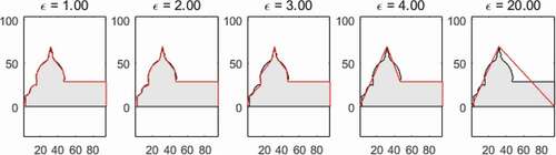
Figure 3. Examples of polygon approximation

A reference shape is one of the primary shapes derived from the original building shape that most fits the original. The concept of utilizing the reference shapes is that firstly, we create the most fitted primary shape to the interest and then discriminate it from the original shape. This idea came from Rosin’s research (2003) and was modified for this study. The most basic definition common to the three primary shapes is on the shape derived from the area of a polygon. Each reference shape of TPS is defined as follows:

• RCA: Reference circle with the same area of the original shape P

• RTA: Reference equilateral triangle with the same area of the original shape P

• RSA: Reference square with the same area of the original shape P

The simplest way to determine discrepancies is to compare two scalar values identified by geometric properties between each reference shape and the original polygon. However, geometric properties that are computed as a single scalar value can cause false equivalence. We adopted the root-mean-square deviation (RMSD), denoted as σ, for an alternative. The RMSD chained together with divergent properties of shapes enables the production of more durable measures. It is one of the most widely used measures (Allen 1971) of the difference between predicted and observed values. The RMSD between the radius and each radial distance (σrR) was normalized so that a perfect basic shape has the maximum value of 1.0, as shown in row C3 in Table 1. The radial distance was substituted with the distance from the centroid to evenly spaced points on the boundary line in C5, considering that the side length of segments varies in most architectural forms. However, it is noteworthy that the effect on RMSD of each deviation between the scalar values and a set of values is proportional to the size of the squared error and sensitive to outliers (Willmott and Matsuura 2006). The consequence implies that a small number of vertices in highly abnormal positions on the polygon significantly affect the destruction of a polygon’s regularity. In other words, long and narrow protrusions, such as cruciform columns towering high above the roof of a church, reduce the overall regularity resulting in a poor shape measurement value when adopting this approach.

When comparing two shapes, it is desirable to observe and resolve locally which parts are identical or not. When two polygons are stacked together, some regions are entirely overlapped together, and some others are exclusively included only in one of the shapes. We adopted Boolean operations on polygons to extract the two polygons’ shared region and unique regions overlaid. Primary operations considered in this study are Union (∪), Intersection (∩), and Exclusive-OR ($\oplus$) presented in Figure 4. When the polygon P1 overlaps from polygon P2, the Union identifies the area belonging to either of them, whereas the intersection detects only the area belonging to both simultaneously. The Exclusive-OR identifies the region that belongs to P1 or P2, but not both. The ratio of the distinct area to the entire area of the two polygons implies the region of the discrepancy between them. Hence, we have expressed the measure of dissimilarity using the operators, such as $\left(P_1\oplus P_2\right)/\left(P_1{\cup }^{P_2}\right)$. The discrimination method of the two sets of shapes has shown a distinguishable performance overall when applied to the measurements of the three primary forms. These operators are specified in International Standard Organization (ISO) and Open Geospatial Consortium (OGC) standard for expressing geospatial relations (Longley et al. 2005). The relevant algorithms can be found in Berg et al. (2008).

Figure 4. Boolean operations of two overlaid polygon

We further investigated the link between the inner angles and shape of each measurement in connection with TPS. It was tricky to use this angle property since the circle and any curved shape share the same characteristics of converging interior angle into the π. Similarly, every inner angle of the square, π/2, shares the same properties with all other orthogonal geometries. Methods induced by modifying RMSD of interior angles between adjacent segments are proposed in the following section but were not very successful at describing the shape precisely enough.

3.2. Circularity measurements

We investigated 13 circularity measurements; some of them were introduced in the previous section. We will discuss each measurement of which the complete mathematical expressions are shown in Table 1. First of all, C1 has a distortion issue caused by an extended perimeter length on the cases with a detailed outline. C2 replaced P with CH, stretching to remove the concave part, and the gap between P and CH is compensated by multiplying the convexity, where the convexity is the proportion of P’s area to CH’s.

More reference circles are adopted for the methods (Sui and Zhang, 2012);

• RCR: The reference circle with the radius of mean radial length, where the radial length is the approximated mean distance from the centroid to the boundary.

• MIC: The maximum inscribed circle.

• MCC: The minimum circumference circle

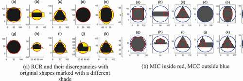
C3 and C4, using reference circle RCA, combine with RMSD and Boolean operators on polygons, respectively. C5 and C6 use RCR similarly: the RCR’s radius is determined by the mean distance between the centroid and each of the evenly distributed points. C7 to C10 use MIC, the largest possible circle inside the polygon and MCC, the smallest possible circle fitted around the polygon. Creating these two reference circles of MIC and MCC of random polygons traditionally have a high computational cost. Although linear time algorithms have been introduced in theoretical mathematics, it is outside the scope of this study to implement the best MIC and MCC generation algorithms in terms of performance. Therefore, the algorithm implemented in this study for the case study is not cost-effective. The C7 is the ratio of the MIC’s radius to the MCC’s radius; the C8 is the ratio of MIC’s area to the object shape P’s area; the C9 is the ratio of MIC’s area to P’s area; the C10 is the ratio of P’s area to the MCC’s area. Figure 5 displays RCR, MIC and MCC on various polygons. We also induced the functions from C11 to C13, based on the hypothesis that the uniform distribution of interior angles of a given polygon close to π makes it look like a circle. However, it turned out to be not exactly right in the experiment, but it related to curvedness where it is not discriminating a circle from ellipses of a variety of eccentricity. Hence, it does not favour the measurement functions related to interior angles, from C11 to C13, as candidates to determine circularities.

Figure 5. Reference circles with variant shapes for the circularity measurements

3.3. Triangularity measurements

We defined eleven triangularity measurements, including the preliminary measures as shown in. T1 is a scalar value computed by the function of (12A√3)/L². It is deduced based on the relations of area and perimeter of the equilateral triangle so that its maximum value becomes 1.0 at an equilateral triangle. To adopt the concept of the reference shape to a triangle, we defined reference triangle RT for a general triangle and RTE for an equilateral triangle. RT is a general triangle to an original shape P. The P’s maximum width determines the base length of RT, and the triangle RT is drawn by connecting the apex of the highest point to both ends of the base, as shown in Figure 6 (a). As RT has no equality constraint which the equilateral triangle has, it is straightforward to apply RT to seek the resemblance to a random triangle. For convenience, the triangularity based on RT was named T2 and measured by the ratio of the P’s area size to the RT’s area size, where the base of the RT is parallel to a horizontal line. T3 was derived by combining characteristics of triangularity and equality from RT and T1. We adopted the discrepancy method for T4 by undertaking the Boolean operations on polygons between RT and P.

Figure 6. (a) RT and (b) RTE of four building facades. (c) RTE and (d) RTA of twelve geometries. The shaded region indicates the discrepancy area while the region filled with solid black indicates the overlapping area

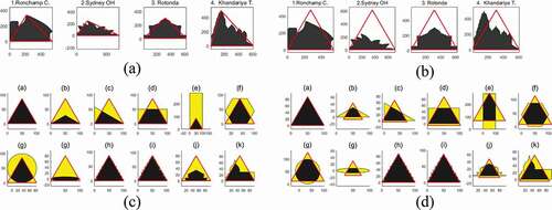
T5 and T6 use RTE, the equilateral triangle whose length is the widest width of P, as shown in Figure 6 (b). T5 is the ratio of the P’s area to the RTE’s, and T6 is the discrepancy area estimated by Boolean operators between them. T7 used the same technique as T6 but with RTA instead. T8 is combined with CH having the T1 value, and the offset between CH and P is cancelled by multiplying by the convexity. Methods from T9 to T11 estimate the triangularities based on vertex angles and symmetry of artificially created side-lines using a line simplification algorithm shown earlier.

3.4. Squareness measurements

Ten squareness and three rectangularity measurement methods are presented in. As discussed earlier in section 3–1, we defined S1 as the function of 16∙A/L² to become 1.0 when the polygon forms a perfect square. Because the side effect of S1 caused by noise and insignificant details bringing extended perimeter can result in distorted measures, S2 is designed to overcome it by taking CH of the P instead of P and multiplying convexity to offset the gap between P and CH.

As rectangles can be viewed as a square variation that deviates from the norm by stretching the height or width, we introduced an axial-aligned bounding box (AABB) for utilizing the rectangularity to approach the squareness assessment. Considering that the building’s base generally corresponds to the horizontal ground, AABB that placed an x-axis parallel to the shape of a building’s ground is suitable as a reference rectangle. AABBs of different shapes are shown in Figure 7 in outermost black broken lines. The rectangularity of R1 computed by P’s area ratio to the AABB’s area provides a way to measure squareness S3. This measurement is defined by multiplying the aspect ratio to R1. A weakness of inflating AABB brought by spikiness of the original shape can cause poor performance in some shapes with sharp protrusions such as church spires.

Figure 7. Reference shapes for the squareness measurements; CH, AABB, RSA, RSD, RRD marked in different line styles

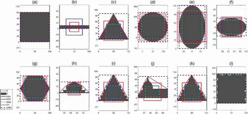
Figure 7 shows the reference squares applied in this study. RSD and RRD were produced in searching for the most fitted square into the shape. Summaries of the reference squares and rectangles utilized in the definition of the squareness measurements are as follows:

• AABB: Axis aligned bounding box

• RSA: Reference square with the same area of the original shape P

• RSD: Reference square, whose side length is the mean horizontal and vertical length.

• RRD: Reference rectangle, whose vertical length is the mean vertical length and the horizontal length is the mean horizontal length across the equally divided intervals at both directions.

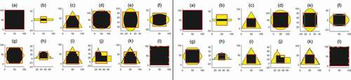
Examples of these reference rectangles and squares are illustrated in Figure 7 with various geometries and architectural buildings. To create RSD and RRD, horizontal and vertical lines that intersect boundary outline are generated at a regular interval, as shown in Figure 8. The mean lengths of these equally distributed horizontal and vertical lines of $\overline{l_x}$ and $\overline{l_y}$ determines the side-length of RSD. S4 is determined by the difference based on RMSD between the side-length of RSA, and horizontal/vertical lengths of the P. S5 is determined in the same manner based on RSD. The expressions in detail are shown in the rows of S4 and S5 in Table 3. RSA and RSD are also utilized in S6 and S7, respectively, with combinations of Polygon Boolean operation. Figure 9 shows the discrepancies computed by Polygon Boolean operation between the reference squares of RSA and RSD and various geometric object shapes over the entire areas of the two polygons stacked together. The reference rectangle RRD with its vertical and horizontal length derived from the mean lengths ($\overline{l_{xi}}$ and $\overline{l_{yi}}$) of P provides the means to measure the rectangularity of R2. S8 is induced by multiplying the aspect ratio to this R2.

Figure 8. The process of building RSD

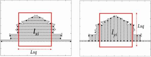
Figure 9. The regions of the exclusive area between RSA and P on the left and RSD and P on the right. The shaded region indicates discrepancy while the solid black indicates the overlapping area

R3 and its derivatives of S9 and S10 are defined under the hypothesis that uniform distributions of the orthogonal angle form a rectangular shape when aliasing is eliminated. The RMSD between each angle of the simplified polygon and orthogonal angle (π/2) is adopted to measure therectangularity of R3 and then applied to measure S9 and S10 but turned out to exhibit a little bit low performance as shown in an experiment coming later.

4. Verifications of the shape measurements

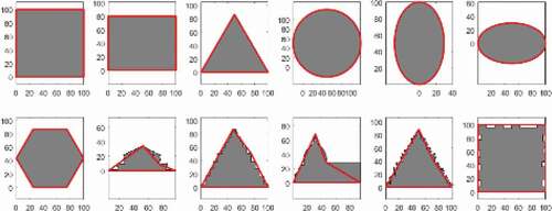
The next step is an evaluation of the proposed measurement methods to compare their performance. A set of deformation models that gradually transform TPS into deforming shapes with a certain degree of variance is devised to verify the shape measurements and present criteria for selecting the best method. Each basic shape steadily transformed into a different shape one by one over iterated steps, from a minimum of 32 steps to a maximum of 64 steps. The degree of deformation was compared with each of the TPS measurements we have defined so far. The best TPS measurement methods are selected based on the correlation between the degree of deformation and the shape measurement’s candidates in each transformation step. Ten deformation models are designed, and thus there are 30 types in total. Each row in Figures 10–12 shows the process of distinctive deformation in a compressed view by selecting intermediate shapes at regular intervals.

Figure 10. Deformations of a reference shape at regular intervals and their correlations with the measures of circularity

The numeric value e, δ, α indicates the degree of deformation estimated independently according to the method of deformation. (* Circularity methods with the highest correlation)

Figure 11. Deformations of a reference shape at regular intervals and their correlations with the measures of triangularity

Figure 12. Deformations of a reference shape at regular intervals and their correlations with the measures of squareness

Estimating the deformation rate during its process to assess the TPS measurements can be as tricky as developing them. Since the amount of variation at each step is likely to be consistent in most cases throughout the entire process, one can say that its serial number in the sequence of transformation refers to the degree of deformation at each level. We can consider the size, or area, of the deformed shape versus the initial underlying shape as a variable representing the degree of deformation when it transforms in the way of shrinking or extending consistently. This estimation is consistent and precise in some cases. When the deformation algorithm is defined mathematically straightforwardly, it is possible to evaluate its geometric attributes. For instance, while the circularity C1 deforms from a perfect circle to an ellipse, the elongation of e gradually increases uniformly at each step. Thus, we use e as the deformation rate so that the correlation of C1 against e value measures the performance of C1. For some transformation models, more sophisticated algorithms are required to generate their deformation degrees. We measure the degree of deformation throughout the entire thirty deformation models using the techniques illustrated already and other evaluation methods designed for each deformation model. Then it is compared with the result of each shape measurement method.

The correlation coefficients between the measurements and the degree of deformation of each type are shown in Tables 4–Table 6. Table 7 presents the average correlation value of all types. The mean values in the tables revealed that all the measurements were highly correlated with the degrees of deformation. However, looking at each TPS measurement for each deformation type in detail, there are significant differences in the correlations between the deformation model types.

Table 4. Correlation coefficients between the measurement methods of circularity and the degrees of deformation with known intervals in a circle

Type	A	B	C	D	E	F	G	H	I	J	Mean R^2
df	32	32	33	32	32	64	60	33	60	60
C1	0.9465	0.8707	0.9166	0.9736	0.9860	0.9345	0.9741	0.9812	0.9867	0.9761	0.9125
C2	0.9465	0.9992	0.9697	1.0000	0.9860	0.9998	0.9953	0.9812	0.9867	0.9993	0.9732
C3	0.9735	0.8284	0.7672	0.9925	0.9261	0.9795	0.9778	0.9938	0.9545	0.9887	0.8857
C4	0.9996	0.9837	0.9953	0.9925	0.9977	0.9859	0.9978	0.9802	0.9951	0.9995	0.9856
C5	0.9990	0.9983	0.9511	0.9908	0.9997	0.9844	0.9946	0.9926	0.9973	0.9986	0.9815
C6	0.9986	0.9769	0.9813	0.9943	0.9984	0.9882	0.9948	0.9831	0.9954	0.9997	0.9823
C7	0.9996	0.9978	0.9992	0.9611	0.9933	0.9855	0.9938	0.9958	0.9955	0.9988	0.9842
C8	0.9995	0.9760	0.9788	0.8147	0.9768	0.9384	1.0000	0.9540	0.9864	0.9954	0.9282
C9	0.9843	0.9572	0.9727	0.8926	0.9483	0.9378	0.9624	0.9907	0.9651	0.9838	0.9214
C10	0.9996	0.9793	0.9951	1.0000	1.0000	1.0000	0.9766	0.9995	0.9986	1.0000	0.9898^(2^)
C11	−0.9382	0.9116	0.9318	0.9059	0.9979	0.9530	0.8941	−0.9970	0.9942	0.9173	0.8927
C12	0.0722^(1)	0.4085	0.9294	0.9592	0.9576	0.7954	0.9463	0.9961	0.9112	0.9149	0.7060
C13	0.8963	0.4095	0.9145	0.9583	0.9575	0.7955	0.9413	0.9961	0.9225	0.9129	0.7838

⁽¹⁾All others are significant at p < 0.01 except this.

⁽²⁾Highest mean of R² (mean R = .9949)

Table 5

Table 5. Correlation coefficients between the measurement methods of circularity and the degrees of deformation with known intervals from an equilateral triangle

Type	A	B	C	D	E	F	G	H	I	J	Mean R^2
df	32	32	32	32	32	32	32	32	32	32
T1	0.9542	0.5592	0.8481	0.9812	0.7926	0.9888	0.9805	0.9143	0.9897	0.4075	0.7454
T2	−0.1814	1.0000	0.9056	0.2706*	1.0000	0.8032	0.9776	0.8452	0.9989	0.9995	0.7238
T3	0.9542	0.9706	0.9804	0.9808	1.0000	0.9505	0.9697	0.8664	0.9989	0.9999	0.9368
T4	0.9542	0.9706	0.9804	0.9808	1.0000	1.0000	0.9697	0.9568	0.9986	0.9985	0.9626
T5	1.0000	1.0000	1.0000	0.9925	1.0000	0.5332	0.9912	0.7122	0.9933	0.9998	0.8745
T6	1.0000	1.0000	1.0000	0.9963	1.0000	0.9955	0.9912	0.9752	0.9977	0.9974	0.9907
T7	0.9949	0.9414	0.9751	0.9906	0.9166	0.9979	0.9893	0.9336	0.9886	0.9977	0.9467
T8	0.9542	0.5592	0.8481	0.9812	0.5106	0.9527	0.9805	0.9873	0.9897	0.9837	0.7957
T9	0.9378	0.9767	0.9958	0.9870	0.9806	0.5162	0.9368	0.9650	0.9800	−0.0749	0.7802
T10	0.9378	0.9767	0.9958	0.9978	0.9806	0.7469	0.9576	0.9197	0.9800	−0.0749	0.8069
GT	0.9542	0.8479	0.9940	0.9816	−0.0118*	0.9788	0.8676	0.9188	0.8111	0.9404	0.7678

1) correlation is significant at the 0.01 level except marked with *

Table 6. Correlation coefficients between the measurement methods of circularity and the degrees of deformation with known intervals from a square

Type	A	B	C	D	E	F	G	H	I	J	Mean R^2
df	32	32	32	32	32	32	32	32	32	32
S1	0.9202	0.9597	1.0000	1.0000	0.9267	0.9851	0.9653	0.9895	0.9141	0.9986	0.9341
S2	0.9202	0.9597	0.9923	0.9922	0.8714	0.9759	0.9715	0.9952	0.9070	0.9982	0.9202
S3	1.0000	1.0000	1.0000	1.0000	0.8319	0.9978	0.9993	0.9973	0.9998	0.9911	0.9663
S4	0.9843	0.9962	0.9066	0.8849	0.9636	0.9914	0.9851	0.9992	0.9898	0.9967	0.9419
S5	0.9843	0.9955	0.9256	0.9245	0.9796	0.9900	0.9849	0.9993	0.9893	0.9948	0.9548
S6	0.9981	0.9733	0.9941	0.9962	0.9863	0.9987	0.9996	0.9952	0.9993	0.9698	0.9823
S7	0.9968	0.9937	0.9822	0.9852	0.9860	0.9988	0.9999	0.9954	0.9991	0.9986	0.9872
S8	1.0000	0.9932	0.9256	0.9559	0.7974	0.9956	0.9996	0.9921	0.9989	0.9862	0.9338
S9	1.0000	0.9995	0.9371	0.9885	0.7525	0.9282	0.9934	0.9884	0.9932	0.9779	0.9189
S10	1.0000	0.9946	0.9404	0.8714	0.7119	0.6711	0.4812	0.5291	0.6976	0.9184	0.6432
R1	−0.0234*	1.0000	1.0000	1.0000	0.8015	0.9995	0.9246	0.9921	0.8082	0.9939	0.9024
R2	0.2575*	0.9955	0.9256	0.9249	0.7879	0.9871	0.9303	0.9918	0.8396	0.9892	0.8701
R3	NA	0.9995*	0.9371	0.9885	0.2072	0.9309	0.7829	0.9897	0.5553	0.9503	0.6961

* all r values except the three marked are significant at p > 0.01, and the values that are not significant at p < 0.01 are excluded from averaging the R² measure.

Table 7. Mean of R squared between the measurement methods and the degrees of deformation

C	C1	C2	C3	C4	C5	C6	C7	C8	C9	C10	C11	C12	C13
mean R^2	0.9125	0.9732	0.8857	0.9856	0.9815	0.9823	0.9842	0.9282	0.9214	0.9898	0.8927	0.706	0.7838
T	T1	T2	T3	T4	T5	T6	T7	T8	T9	T10	GT
mean R^2	0.7454	0.7238	0.9368	0.9626	0.8745	0.9907	0.9467	0.7957	0.7802	0.8069	0.7678
S	S1	S2	S3	S4	S5	S6	S7	S8	S9	S10	R1	R2	R3
mean R^2	0.9341	0.9202	0.9663	0.9419	0.9548	0.9823	0.9872	0.9338	0.9189	0.6432	0.9024	0.8701	0.6961

Most circularity measurements show good performance. Again, exceptions arise in specific transformation methods determined by curvatures, such as C11, C12 and C13. C11 shows a negative correlation with Type A and H (Table 4). The former transforms into an ellipse with a high degree of elongation, while the latter transforms a circle into a square. C12 and C13 have eminently low correlations of 0.4085 and 0.4095 in Type B, respectively, which mutate into star shapes in Triangularity has exceptional cases for several measurement methods, as shown in. Type-J shows no correlations with T9 and T10 at each level. Types B and E show a low correlation of 0.5592 and 0.5106 with T8, as highlighted in the table. When the shape deformations of Type B and E are examined, the triangle gradually grows into a column while turning the vertices on both sides of the triangle into lines in Type B. The base gradually grows into the square, covering the apex of the triangle in Type-E. Although these exceptional cases exist depending on the deformation types, their consistent variation is handled well in many measurement methods, such as T2, T3, T4, T5 and T6. The highest correlation reaches its maximum value of 1.0. Most of the squareness measurements also show remarkably high performance, except for S10 (mean squared R is 0.6432) measured by its angle, as shown in Table 6. Based on the highest mean correlation coefficients between the strains and the measurements for the experiments, as shown in Table 7, we have chosen the methods of C10, T6 and S7 as final shape descriptors to employ in the analysis of 60 building shapes followed in the next chapter.

As a secondary descriptor, we define “deformity” simultaneously to describe the intensity of deviation from all the TPS as the function of. Its application to thirty buildings is illustrated in Table 8. This index indicates that how far away a building shape is from all of the attributes of TPS. The shape descriptor clearly shows the geometric differences between building shapes. It is not based on topologic ideas but rooted in the pure forms in architectural design. For architects who are very keen to produce certain forms, the first step is to understand their geometric properties and then catch their differences intuitively. This measure makes it possible for them to know where their designs are placed between rigid and non-rigid shapes or between geometric and free-form ones. Based on this, the designers could manipulate and confirm their designs in various ways to create a proper form of what they intend in terms of purely architectural forms.

Table 8. Shape measurements of 30 buildings classified into two types of shapes

Building	Facade Floor pl.	Circularity	Equilateral triangularity	Squareness	Deformity	Dominant shape	Dominance	Percentage difference with mean dominance
Ronchamp Chapel	Facade	0.5334	0.7130	0.5526	0.4003	ET	0.1133	19.43
	Floor Pl.	0.4911	0.5723	0.6477	0.4296	S	0.0773	21.39
Sydney Opera House	Facade	0.2151	0.3760	0.3981	0.6703	S	0.0684	30.73
	Floor Pl.	0.5452	0.5693	0.5890	0.4322	S	0.0212	93.67
Villa Rotonda, Vicenza	Facade	0.3590	0.6293	0.5247	0.4957	ET	0.1250	29.11
	Floor Pl.	0.7917	0.4400	0.6958	0.3575	C	0.1492	43.60
Temple of Khandariya Mahadeo, Khajuraho	Facade	0.3717	0.5784	0.4575	0.5308	ET	0.1092	15.77
	Floor Pl.	0.3671	0.4866	0.5350	0.5371	S	0.0721	26.78
Taj Mahal, Agra	Facade	0.4639	0.6362	0.5345	0.4551	ET	0.0913	2.10
	Floor Pl.	0.7811	0.4356	0.9326	0.2836	S	0.2162	121.27
Villa Savoye, Dessau	Facade	0.4290	0.5776	0.4678	0.5085	ET	0.0861	7.96
	Floor Pl.	0.7399	0.5533	0.8296	0.2924	S	0.1220	23.49
Tokyo Olympic Hall, Tokyo	Facade	0.1850	0.3139	0.3793	0.7073	S	0.0866	7.38
	Floor Pl.	0.3146	0.5352	0.5578	0.5308	S	0.0886	12.35
North Christian Church	Facade	0.1715	0.4743	0.1994	0.7183	ET	0.1926	69.52
	Floor Pl.	0.6537	0.6019	0.6836	0.3536	S	0.0372	42.99
Guggenheim Museum, Bilbao	Facade	0.1406	0.2469	0.2532	0.7864	S	0.0396	80.76
	Floor Pl.	0.2903	0.4575	0.3359	0.6388	ET	0.0963	5.48
Mt. Angel Abbey Library, St. Benedict	Facade	0.2497	0.3506	0.4686	0.6437	S	0.1123	18.55
	Floor Pl.	0.4312	0.6649	0.6161	0.4293	ET	0.0942	5.58
Pantheon, Rome	Facade	0.6938	0.6204	0.7615	0.3081	S	0.0696	29.03
	Floor Pl.	0.5176	0.5766	0.6323	0.4245	S	0.0568	51.05
Mingtang-Biyong Ritual Complex, Xian	Facade	0.3925	0.6799	0.5633	0.4548	ET	0.1347	36.38
	Floor Pl.	0.8108	0.4400	0.7781	0.3237	C	0.1345	29.28
St. Michael, Hildesheim	Facade	0.3788	0.5621	0.4286	0.5435	ET	0.1056	12.44
	Floor Pl.	0.4367	0.5014	0.5062	0.5186	S	0.0248	73.23
Great Stupa, Sanchi	Facade	0.2697	0.4837	0.5348	0.5706	S	0.1054	12.25
	Floor Pl.	0.7461	0.4557	0.5977	0.4002	C	0.1463	44.93
Philharmonic Hall, Berlin	Facade	0.3675	0.6092	0.5171	0.5021	ET	0.1113	17.66
	Floor Pl.	0.6072	0.4926	0.7852	0.3717	S	0.1569	53.70
Price Tower, Oklahoma	Facade	0.3250	0.1587	0.3810	0.7118	S	0.0928	0.47
	Floor Pl.	0.6624	0.5714	0.6881	0.3594	S	0.0475	54.56
Blues Point Tower, Sydney	Facade	0.3279	0.1299	0.3705	0.7239	S	0.0944	1.24
	Floor Pl.	0.6339	0.4747	0.9139	0.3258	S	0.2397	143.50
Nexus World Housing (Steven Hall), Fukuoka	Facade	0.2859	0.4441	0.3140	0.6520	ET	0.0961	3.02
	Floor Pl.	0.2547	0.3690	0.2979	0.6928	ET	0.0618	39.06
The Whale, Amsterdam	Facade	0.3103	0.4514	0.3442	0.6314	ET	0.0828	11.86
	Floor Pl.	0.3365	0.2755	0.2984	0.6965	C	0.0330	73.39
Leicester Univ. Eng. Bldg., Leicester	Facade	0.4708	0.7255	0.4998	0.4346	ET	0.1601	52.79
	Floor Pl.	0.6315	0.6326	0.6324	0.3678	ET	0.0004	76.65
Arab World Institute, Paris	Facade	0.4672	0.6014	0.4911	0.4801	ET	0.0815	13.43
	Floor Pl.	0.3248	0.4790	0.4121	0.5947	ET	0.0737	29.10
London City Hall, London	Facade	0.5069	0.6243	0.6900	0.3929	S	0.0829	11.74
	Floor Pl.	0.9974	0.4337	0.7367	0.2774	C	0.2748	190.87
Mercedes-Benz Museum, Stuttgart	Facade	0.5485	0.6230	0.6499	0.3929	S	0.0428	74.15
	Floor Pl.	0.7267	0.5789	0.6675	0.3423	C	0.0690	43.56
30 St. Mary Axe, London	Facade	0.3196	0.1604	0.4172	0.7009	S	0.1181	23.53
	Floor Pl.	0.9927	0.4360	0.7393	0.2773	C	0.2700	155.69
Seattle Library, Seattle	Facade	0.5260	0.6958	0.7770	0.3337	S	0.1107	17.13
	Floor Pl.	0.6322	0.4873	0.8916	0.3296	S	0.2212	114.86
Hu-Tong House (Waro Kishi), Japan	Facade	0.2774	0.3959	0.3194	0.6691	ET	0.0650	35.69
	Floor Pl.	0.5027	0.5016	0.5849	0.4703	S	0.0552	54.41
Federal Environmental Agency, Dessau	Facade	0.0697	0.1245	0.1108	0.8983	ET	0.0228	121.40
	Floor Pl.	0.1829	0.2208	0.2333	0.7877	S	0.0210	128.74
de Young Museum, San Francisco	Facade	0.1735	0.2607	0.2055	0.7868	ET	0.0475	65.00
	Floor Pl.	0.5005	0.6006	0.5954	0.4345	ET	0.0351	88.10
Des Moines Public Library, Iowa	Facade	0.1568	0.2625	0.1896	0.7970	ET	0.0595	44.18
	Floor Pl.	0.2228	0.3554	0.2537	0.7227	ET	0.0781	27.60
Kunsthaus, Austria	Facade	0.3450	0.5258	0.4393	0.5633	ET	0.0891	4.54
	Floor Pl.	0.5456	0.5000	0.5674	0.4623	S	0.0297	74.44
Mean	Facade	0.3444	0.4679	0.4413	0.5821	-	0.0932	28.98
	Floor Pl.	0.5572	0.4899	0.6078	0.4488		0.1001	64.78
	Total	0.4501	0.4789	0.5246	0.5155		0.0967	46.88

An index of “dominance” can be computed as the function of      to see how much the shape with maximum TPS measurement is dominant in a building form. This index is particularly beneficial to researchers seeking out the questions in a manner of quantitative measurements: why do a specific form prevail in a building design? Moreover, how dominant is it? Which descriptor is it among the TPS? They also may raise a question of how symbolic a building shape of a façade or floor plan is? The measure of “dominance” may serve as a valuable index to answer those questions and clarify a general trend of a shape awareness objectively resided in building design. These two second-level descriptors are shown in columns to the right of each measurement value in Table 8, along with the most dominant shape using the acronym C for circularity, S for squareness, and ET for equilateral triangles.

5. Case study

The measurement methods introduced are applied to 30 well-known historic buildings, as shown in Table 8. A total of 60 building shapes of front side façades and their floor plans were collected from the books written by Gregory (2008) and Stierlin (1994). These images were converted into digital format (DXF) in Matlab to extract the coordinates of polygons. Pairs of façade silhouettes and corresponding floor plan outlines are shown with measured values in Figures 13–15. Buildings are numbered from 1 to 30.

Figure 13. Circularity measured using the C10 method with reference circle MCC

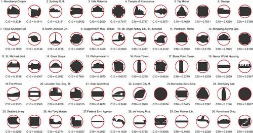
Figure 14. Triangularity measured using the T6 method with the reference equilateral-triangle RET

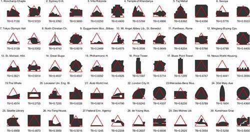
Figure 15. Triangularity measured using the T6 method with the reference equilateral-triangle RET

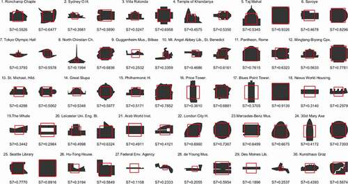
Analyzing the measurement results of the facade shapes shown in these figures, the Ronchamp Chapel has a protruding roof in the middle, resulting in triangularity predominance as a value of 0.7130. At the same time, the relatively constant aspect ratio does not significantly destroy the circularity and squareness whose properties contain regularity. The facade shape of the North Christian Church has a circularity of 0.1715, and its triangularity and squareness are 0.4743 and 0.1994, respectively. The massive gaps from the reference geometry due to high-rise spires lower all three measurement values. However, it is convincing that the relatively high triangularity compared to other shape descriptors confirms how the building façade is perceived in general.

On the other hand, as the outline of the Ronchamp Chapel’s floor plan has a part of the entrance wall sharply protruding, it seems to make its shape a little bit ambiguous in terms of the TPS to bare eyes. Its circularity is 0.4911, and triangularity and squareness are 0.5723 and 0.6477, respectively, which is matched to fit a more square form. However, it embarrasses us that some other floor plans do not match our institutional expectations. The floor plan of the Tokyo Olympic Hall shows the most striking example; it shows less circularity at 0.3146 than squareness (0.5578) and triangularity (0.5352). Its central area of the circular shape let us expect to obtain a higher circularity among the three descriptors. However, the considerable gap with MCC caused by protrusions on both winged sides, which brings much lower circularity than expected, and deviates from our expectations. In these exceptional cases, it seems more appropriate to employ one of the circularities of C4, C5 or C6, because these measurements utilize the reference circles of which the radius is closer to the average distances from the centre of the shapes, such as RCR and RCA. The correlations of these circularities showing 0.9856 in C4, and 0.9815 and 0.9823 in C5 and C6, respectively, are almost as high as C10.

Regarding the performance of the two second-level descriptors, the Guggenheim Museum Bilbao, for example, shows much higher deformity as a value of 0.7864 than the Ronchamp Chapel’s 0.4006 as summarized in Table 8. Likewise, any average strain that deviated from the TPS of a building can be quantitatively identified and compared to other buildings by examining each deformity value. A triangle works as the most dominant shape in the façade of the chapel with a value of 0.1133, while a square is the prevalent one in the museum with 0.0396. This difference in the dominance index as a value of 0.073 seems significant, considering that the median of the 60 shapes is 0.0967. It could be understood that the chapel’s façade maintains some more rigid triangular shape in general with the intensity of 0.1133 while that of the museum does not allow to imagine a particular type of form as low as 0.0396, ranking ninth out of sixty. The disparity of 0.0737 between the two values seems trivial, but it becomes noteworthy if the difference is expressed as a percentage. It shows a percentage of 96.40 computed by dividing the difference by the average of two values (Δv/(Σv/2)). Based on this calculation, the chapel’s façade is dominated by a triangle at a strength of 19.43% compared to the average of the 30 façade shapes. Meanwhile, the museum shows a lower strength of 80.76%.

It is particularly noteworthy that Table 8 presents an in-depth clue for the quantitatively proofed difference inherent in the shapes of façades and floor plans. Considering the difference of deformities between the means of two types of shapes, the facade shows a value of 0.5821 while the floor plan is 0.4488. This difference could be understood in that the facades prioritize the visual experience while the floor plans represent the importance of the spatial arrangement by somewhat stereotypical layouts. By applying and exploring the above-disclosed shape descriptors, it will be possible to grasp buildings’ morphological characteristics for each type, purposes, locations , and cultural difference of the buildings. Although these measurements are limited in their comparisons and evaluations of architectural shape to the features of the three primary shapes, we expect to objectively demonstrate the shape awareness inherent in the building designs by comparing and evaluating the architectural shapes.

6. Conclusion

Grasping the difference between building forms in the traditional geometry terms has become an urgent issue as the architects have a powerful tools, such as Catia, which makes it possible to realize free-form designs in the real world. Hence, our question directly comes from the issue of how we can capture the geometric difference with other forms, for example, the difference of façade shapes between the Ronchamp Chapel and the Guggenheim Museum Bilbao. This quantitative verification serves as the criteria for confirming their building forms’ whereabouts. The three primary shapes of circle, triangle and square have been regarded as the criteria for judging the whereabouts of building forms across the spectrum of Euclidean geometry in its classical sense. This study has shown a way to explicitly designate a building’s form by combining the parameters of the three primary shapes, just as when referring to color with the combination of hue, saturation and brightness or light with RGB values rather than its ambiguous adjectives.

Based on the primary shapes as the criteria, this study explored the shape measurement methods of circularity, triangularity and squareness. For this, we employed a well-known geometric property of the ratio of area to length to measure the proximity of the given shape to the three primary shapes. As it became clear that the jaggedness of the shapes’ outlines affected this ratio, we applied the straightening and simplifying techniques to the ratio to redeem the distortion. Based on the shape measures of similarity, we introduced various reference shapes to compare with the given building shapes. We adopted two different approaches to compare the two types of reference and designated shapes; one was a statistical method of RMSD and the other Boolean operations on polygons. The next step was evaluating the validity of the proposed measurement methods and discriminating between their performances. This evaluation led to the development of a progressive deformation program, iterating slight changes in each step. The iteration was not noticeable by step but completely destructed in a final one.

This study could finally propose the three measurement methods as follows: a circularity of C10 measured by the ratio of P’s area to the MCC’s, a triangularity of T6 incorporating RTE and the discrepancy area estimated by Boolean operators on polygons between the two types of shapes and a squareness of S7 utilizing RSD with the combination of Boolean operations. We chose each of the three measurement methods showing the highest correlation coefficients between the changes of deformation at each step of iterations that we already knew and the shape measurements of similarity between a given form and a reference one. A good correlation was observed in most cases with some exceptions, which could be interpreted to allow flexible use of the measurement methods. The three measurement methods produced second-level shape descriptors of “deformity” and “dominance”. They were tested with 60 shapes consisting of the facades and floor plans of 30 buildings.

The results revealed that squareness was the most dominant shape property, and triangularity and circularity followed. The squareness became even more visible as a mean of 0.6078 when we counted the floor plans only. This high figure confirmed why the square or rectangular shape prevails in the floor plans, as Steadman (2006) reported. It was also noteworthy to find out that the façade shape was more deformed than the floor plans. This difference in this deformity was undoubtedly regarded as the explicit evidence of why the façade looked somewhat free in its shape formation. At the same time, the floor plan was more oriented towards its functional aspects. This interpretation could be supported by the difference of dominance values, in which a specific primary shape dominates the floor plans with high values than the facades did in general. The results could draw attention from researchers and architects who are serious about building forms’ design judgment. It is, therefore, reasonable to anticipate that this study stimulates the development of other shape descriptors that make it possible for them to verify the geometric properties of their design forms and eventually lead to their enhancement.

This study had several limitations: First, the problem of choosing the best measurements out of all the proposed methods is a delicate matter since there are minor differences in their correlation coefficients. This difficulty, therefore, brings out other parameters, such as the purpose of measurement, run-time complexity of the algorithm, and cost of implementation rather than the negligible differences observed in the performance. Nevertheless, we chose the three methods of C10, T6, and S7 for the strictness of the experiment in the case study because the most straightforward strategy of choosing only one of all the methods would be to select that with the highest mean of the correlation values between the strains and the measured values. However, the downside of choosing C10 as the most justifiable circularity measure was that computing MCC of irregular non-convex building shapes was not trivial on computational complexity. Thus, it is reasonable to replace it by selecting other methods that ignore the negligible performance differences depending on the environment of shape analysis. Comparable results, for example, can be attained by replacing C10 with C4 using a reference circle RCA that can be drawn more straightforwardly and cost-effectively. We leave these issues for further work as we focus on the geometric difference of architectural forms in the three primary shapes.

Acknowledgments

This study was supported by a research fund from Chosun University (2019).

Disclosure statement

We wish to confirm that there are no known conflicts of interest associated with this publication and there has been no significant financial support for this work that could have influenced its outcome. We confirm that the manuscript has been read and approved by all named authors and that there are no other persons who satisfied the criteria for authorship but are not listed. We further confirm that the order of authors listed in the manuscript has been approved by all of us. We confirm that we have given due consideration to the protection of intellectual property associated with this work and that there are no impediments to publication, including the timing of publication, with respect to intellectual property. In so doing, we confirm that we have followed the regulations of our institutions concerning intellectual property.

Additional information

Funding

This work was supported by the Chosun University [2019].

Notes on contributors

Dongkuk Chang

Dongkuk Chang received his Ph.D. in architecture from the Bartlett School of Architecture and Planning at the University College London and is currently a professor in the Center for the Design of Architectural Space Structure (Cdass) of the School of Architecture at Chosun University in South Korea.

Joohee Park

Joohee Park received his Msc in Advanced Computing from the University of London by King's College London and had been working on the field of computer programming for many years and currently a researcher at Chosun University in South Korea.

References

- Allen, D. M. 1971. “Mean Square Error of Prediction as a Criterion for Selecting Variables.” Technometrics 13 (3): 469–475. doi:https://doi.org/10.1080/00401706.1971.10488811.
- Arnheim, R. 1974. Art and Visual Perception: A Psychology of the Creative Eye. Berkeley, California: University of California Press.
- Bar, M., and M. Neta. 2006. “Humans Prefer Curved Visual Objects.” Psychological Science 17 (8): 645–648. doi:https://doi.org/10.1111/j.1467-9280.2006.01759.x.
- Batty, M. 2001. “Exploring Isovist Fields: Space and Shape in Architectural and Urban Morphology.” Environment and Planning B: Planning and Design 28: 123–150. doi:https://doi.org/10.1068/b2725.
- Bemis, A. F., and J. Burchard. 1933-36. The Evolving House. Vol. 3. Boston: Technology Press, MIT.
- Benedikt, M. L. 1979. “To Take Hold of Space: Isovist and Isovist Field.” Environment and Planning B: Planning and Design 6 (1): 47–65. doi:https://doi.org/10.1068/b060047.
- Benedikt, Michael L 3 1979/3 To take hold of space: isovists and isovist fields Environment and Planning B: Planning and design 6 1 47–65
- Berg, M., O. Cheong, M. J. Kreveld, and M. H. Overmars. 2008. Computational Geometry: Algorithms and Applications. 3rd ed. Berlin: Springer.
- Berlyne, D. E. Aesthetics and psychobiology (New York: Appleton-Century-Crofts)
- Biederman, I., and G. Ju. 1988. “Surface versus Edged-based Determinants of Visual Recognition.” Cognitive Psychology 20 (1): 38–64. doi:https://doi.org/10.1016/0010-0285(88)90024-2.
- Bingham, H. C. 1914. “A Definition of Form.” Journal of Animal Behavior 4 (2): 136–141. doi:https://doi.org/10.1037/h0075660.
- Birkhoff, G. D. 1933. Aesthetic Measure. Cambridge, MA: Harvard University Press.
- Bone, P. 2021. “Polygon Simplification.” MATLAB Central File Exchange. Accessed 21 June 2021. https://www.mathworks.com/matlabcentral/fileexchange/45342-polygon-simplification
- Brachmann, A., and C. Redies. 2017. “Computational and Experimental Approaches to Visual Aesthetics.” Frontiers in Computational Neuroscience 11: 102. doi:https://doi.org/10.3389/fncom.2017.0010211.
- Brown, D., and D. Owen. 1967. “The Metrics of Visual Form: Methodological Dyspepsia.” Psychological Bulletin 68 (4): 243–259. doi:https://doi.org/10.1037/h0025037.
- Chen H and Rokne J. 1992. The convex hull of a set of convex polygons. International Journal of Computer Mathematics, 42(3–4), 163–172. https://doi.org/10.1080/00207169208804059
- Ching, F. 2007. Architecture: Form, Space, and Order. 3rd ed. Hoboken, NJ: John Wiley and Sons.
- Conroy, R. 2000. “Spatial Navigation in Immersive Virtual Environments.” PhD thesis, University College London.
- Douglas, D., and T. Peucker. 1973. “Algorithms for the Reduction of the Number of Points Required to Represent a Digitized Line or Its Caricature.” Cartographica: The International Journal for Geographic Information and Geovisualization 10 (2): 112–122. doi:https://doi.org/10.3138/FM57-6770-U75U-7727.
- Eu, D., and G. Toussaint. 1994. “On Approximating Polygonal Curves in Two and Three Dimensions.” CVGIP: Graphical Models and Image Processing 56 (3): 231–246. doi:https://doi.org/10.1006/cgip.1994.1021.
- Eysenck, H J. 1942. The appreciation of humour: An experimental and theoretical study. British Journal of Psychology. General Section, 32(4), 295–309. https://doi.org/10.1111/j.2044-8295.1942.tb01027.x
- Fellow, B. 1968. The Discrimination Process and Development. Exter: Pergamon Press.
- Franz, G., and J. M. Wiener. 2008. “From Space Syntax to Space Semantics: A Behaviorally and Perceptually Oriented Methodology for the Efficient Description of the Geometry and Topology of Environments.” Environment and Planning B: Planning and Design 34 (4): 574–592. doi:https://doi.org/10.1068/b33050.
- Gellermann, L. W. 1933. “Chance Orders of Alternating Stimuli in Visual Discrimination Experiments.” The Pedagogical Seminary and Journal of Genetic Psychology 42 (1): 206–208. doi:https://doi.org/10.1080/08856559.1933.10534237.
- Gordon, P. 2004. “Numerical Cognition without Words: Evidence from Amazonia.” Science 306 (5695): 496–499. doi:https://doi.org/10.1126/science.1094492.
- Greenfield, G. 2005. “On the Origins of the Term Computational Aesthetics.” Proceedings of the First Eurographics Conference on Computational Aesthetics in Graphics, Visualization and Imaging, Girona: Eurographics Association, 9–12.
- Gregory, R. 2008. Key Contemporary Buildings. New York: W.W. Norton & Company, Inc.
- Helmholtz, H. von. 1924. Physiological optics (Transl. by J.P.C. Southall). Rochester, New York: Optical Society of America
- Hillier, B., and J. Hanson. 1984. The Social Logic of Space. Cambridge: Cambridge University Press.
- Holmyard, E. J. 1957. Alchemy. Edinburgh: Penguin Books.
- Iigaya, K., S. Yi, I. A. Wahle, K. Tanwisuth, and J. P. O’Doherty. 2021. “Aesthetic Preference for Art Can Be Predicted from a Mixture of Low- and High-level Visual Features.” Nature Human Behaviour 5: 743–755. doi:https://doi.org/10.1038/s41562-021-01124-6.
- Jung, C. G. 1964. Man and His Symbol. New York: Doubleday and Co.
- Jung, C. G. 1968. Psychology and Alchemy. 2nd ed. Princeton: Princeton University Press.
- Kellogg, R. 1970. Analyzing Children’s Art. Palo Alto, CA: National Press Books.
- Kim, T., W. Bair, and A. Pasupathy. 2019. “Neural Coding for Shape and Texture in Macaque Area V4.” The Journal of Neuroscience 39 (24): 4760–4774. doi:https://doi.org/10.1523/JNEUROSCI.3073-18.2019.
- Krüger M J. 1979. An approach to built-form connectivity at an urban scale: system description and its representation. Environ. Plann. B, 6(1), 67–88. https://doi.org/10.1068/b060067
- Lenartowicz, J. K. 2014. “Equilateral Triangle and the Holy Trinity.” Journal of Architecture and Urbanism 38 (4): 220–233. doi:https://doi.org/10.3846/20297955.2014.994807.
- Lindal, P. J., and T. Hartig. 2013. “Architectural Variation, Building Height, and the Restorative Quality of Urban Residential Streetscapes.” Journal of Environmental Psychology 33: 26–36. doi:https://doi.org/10.1016/j.jenvp.2012.09.003.
- Longley, P., M. Goodchild, D. Maguire, and D. Rhind. 2005. Geographical Information Systems and Science. Chichester: John Wiley & Sons.
- Luebke, D. 2001. “A Developer’s Survey of Polygonal Simplification Algorithms.” IEEE Computer Graphics and Applications 21 (3): 24–35. doi:https://doi.org/10.1109/38.920624.
- Lupton, E., and J. A. Miller. 1991. The Bauhaus and Design Theory (Korean Translated Edition 1996, Kukje Publishing House). New York: Princeton Architectural Press.
- Metzger, W. 2006. Laws of Seeing. Cambridge, MA: MIT Press.
- O’Rourke, J. 1998. Computational Geometry in C. 2nd ed. Cambridge: Cambridge University Press.
- Oikonomou, A. 2021. “The Use of Geometrical Tracing, Module and Proportions in Design and Construction, from Antiquity to the 18th Century.” International Journal of Architectural Heritage: 1–21. 202103290. doi:https://doi.org/10.1080/15583058.2021.1899339.
- Pasupathy, A., Y. El-Shamayleh, and D. V. Popovkina. 2019. “Visual Shape and Object Perception.” Oxford Research Encyclopedia of Neuroscience. doi:https://doi.org/10.1093/acrefore/9780190264086.013.75.
- Piaget, J., and B. Inhelder. 1956. The Child’s Conception of Space. London: Routledge and Kegan Paul.
- Rebe, R., N. Schwarz, and P. Winkielman. 2004. “Processing Fluency and Aesthetic Pleasure: Is Beauty in the Perceiver’s Processing Experience?” Personality and Social Psychology Review 8 (4): 364–382. doi:https://doi.org/10.1207/s15327957pspr0804_3.
- Redies C. A universal model of esthetic perception based on the sensory coding of natural stimuli. Spatial Vis, 21(1–2), 97–117. https://doi.org/10.1163/156856807782753886
- Rosin, P. L. 2003. “Measuring Shape: Ellipticity, Rectangularity, and Triangularity.” Machine Vision and Applications 14 (3): 172–184. doi:https://doi.org/10.1007/s00138-002-0118-6.
- Schneider, M. S. 1995. A Beginner’s Guide to Constructing the Universe: Mathematical Archetypes of Nature, Art, and Science. New York: Harper.
- Seeley, I. H. 1983. Building Economics. 3rd ed. London: Macmillan.
- Smock, W. 2004. The Bauhaus Ideal, Then and Now. Chicago: Academy Chicago Publishers.
- Stamps, A. E. 1999. “Physical Determinants of Preferences for Residential Facades.” Environment and Behavior 31 (6): 723–751. doi:https://doi.org/10.1177/00139169921972326.
- Stamps, A. E. 2000. Psychology and the Aesthetics of the Built Environment. New York: Kluwer Academic/Plenum Publishers.
- Steadman, P. 2006. “Why are Most Buildings Rectangular?” ARQ: Architectural Research Quarterly 10 (2): 119–130. doi:https://doi.org/10.1017/S1359135506000200.
- Steadman, P. 2014. “.” In Building Types and Built Forms. Leicestershire: ,Matador.
- Stierlin, H. 1994. Encyclopedia of World Architecture. Cologne: Benedikt Taschen.
- Sui, W., and D. Zhang. 2012. “Four Methods for Roundness Evaluation.” Physics Procedia 24 (Part C): 2159–2164. doi:https://doi.org/10.1016/j.phpro.2012.02.317.
- Vartanian, O., G. Navarrete, A. Chatterjee, L. B. Fich, H. Leder, C. Modrono, M. Nadal, N. Rostrup, and M. Skov. 2013. “Impact of Contour on Aesthetic Judgments and Approach-avoidance Decisions in Architecture.” Proceedings of the National Academy of Sciences 110 (Supplement_2): 10446–10453. doi:https://doi.org/10.1073/pnas.1301227110.
- Willmott, C. J., and K. Matsuura. 2006. “On the Use of Dimensioned Measures of Error to Evaluate the Performance of Spatial Interpolators.” International Journal of Geographical Information Science 20 (1): 89–102. doi:https://doi.org/10.1080/13658810500286976.
- Wing, C. K. 1999. “On the Issue of Plan Shape Complexity: Plan Shape Indices Revisited.” Construction Management and Economics 17 (4): 473–482. doi:https://doi.org/10.1080/014461999371394.
- Witkin, A. P., and J. M. Tenenbaum. 1983. “On the Role of Structure in Vision.” In Human and Machine Vision, edited by J. Beck, B. Hope, and B. Rosenfeld. New York: Academic Press 481–543 .
- Yılmaz, S., H. Özgüner, and S. Mumcu. 2018. “An Aesthetic Approach to Planting Design in Urban Parks and Greenspaces.” Landscape Research 43 (7): 965–983. doi:https://doi.org/10.1080/01426397.2017.1415313.
- Zhang, D., and G. Lu. 2004. “Review of Shape Representation and Description Techniques.” Pattern Recognition 37 (1): 1–19. doi:https://doi.org/10.1016/j.patcog.2003.07.008.
- Zusne, L. 1965. “Moments of Area and of the Perimeter of Visual Form as Predictors of Discrimination Performance.” Journal of Experimental Psychology 69 (3): 213–220. doi:https://doi.org/10.1037/h0021735.
- Zusne, L. 1970. Visual Perception of Form. New York: Academic Press.