Optimizing reinforced concrete beams cost based on AI-based Lagrange functions

ABSTRACT

This study aims to develop artificial neural networks (ANNs)-based forward Lagrange networks optimizing ductile doubly reinforced concrete (RC) beams. Cost (CI_b) of materials and manufacture were established as an objective function, which is minimized considering constraints according to engineer’s needs. Large datasets of 100,000 were used to derive an AI-based objective function for cost (CI_b, minimizing cost of an RC beams) as a function of forward input parameters, replacing complex analytical objective functions. A resilient design capable of finding concrete beams beyond human efficiency is based on equality and inequality constraints, which are implanted in AI-based Lagrange. Optimal designs are not simple especially when multiple constraining conditions are to be considered. Neither is it possible for engineers to pre-assign constraining conditions which can be sequentially calculated in an output of a conventional design. Cost of RC beams minimized by forward Lagrange networks was reduced 18%–26% compared to probable beam designs. AI-based design charts with eight forward outputs (ϕM_n,M_u,M_cr,ε_{rt_0.003},ε_{rc_0.003},Δ_imme,Δ_long,CI_b) based on nine forward inputs (L, h, b, f_y,f^’_c, ρ_rt,ρ_rc,M_D,M_L) are proposed to assist engineers to design ductile doubly RC beams, presenting minimized CI_b in the preliminary design stage.

Graphical Abstract

KEYWORDS:

• Artificial neural networks
• doubly reinforced concrete beams
• lagrange multiplier method
• optimization design charts
• random design range

1. Introduction: current research, significance, and ideology of the proposed methodology

Some optimization studies have been performed widely in civil and architectural engineering, particularly in optimizing reinforced concrete (RC) structures (Aghaee, Yazdi, and Tsavdaridis 2014; Fanaie, Aghajani, and Dizaj 2016; Madadi et al. 2018; Nasrollahi et al. 2018, and Paknahad, Bazzaz, and Khorami 2018). Most of these studies only focused on minimizing the manufacturing and construction costs. Structural capabilities should be taken into consideration against external forces, which are controlled by design codes. Several optimization methods of RC beam have been performed successfully by (Shariati et al. 2010; Fanaie, Aghajani, and Shamloo 2012; Toghroli et al. 2014; Awal, Shehu, and Ismail 2015; Kaveh and Shokohi 2015; Safa et al. 2016; Shah et al. 2016; Korouzhdeh, Eskandari-Naddaf, and Gharouni-Nik 2017, and Heydari and Shariati 2018). Shariat et al. (2018) established the cost of frames as an analytical objective function of the design parameters; however, the analytical objective functions, which represent the entire behavior of structural components, are generally hard to be derived. A procedure, therefore, to achieve approximate objective functions based on artificial neural networks (ANNs) was proposed in this study.

ANNs were kept being implemented in the field of structural engineering. Rizzo and Caracoglia (2020) proposed a procedure to predict a critical flutter velocity of suspension bridges with closed box deck sections based on the implementation of an ANN. Gomes et al. (2019) proposed to apply ANN on predicting delamination failure in carbon fiber reinforcement polymer (CFRP) plates. A feed-forward-based neural network was used to detect damage based on big data obtained from finite element analysis (FEA), then results based on ANN were verified by numerical algorithms. They stated that ANN was an effective tool for delamination damage identification problem. Flood and Kartam (1994a, 1994b) presented a concept and an application of neural networks to structural engineering by exploring an influence of number of hidden layers and nodes on the validation of network, and processing speed for deep learning networks. They concluded that success of a neural network implementation is dependent on a quality of data used for training. Hong (2019) also investigated the influence of a number of training datasets on training accuracies. Wu and Jahanshahi (2019) proposed CNN approach to better predict the structural responses compared with the multiple layer perceptron (MLP) algorithm against noisy data. They presented a deep convolutional neural network (CNN)-based approach to estimate dynamic response of a linear single-degree-of-freedom (SDOF) system, a nonlinear SDOF system, and a full-scale 3-story multi-degree of freedom (MDOF) steel frame. Ahmadi, Moghadas, and Lavaei (2008) presented back-propagation wavelet neural network (BPW) based on scaled conjugate gradient (SCG) algorithm, which replaced sigmoid activation functions of hidden layer neurons by wavelets to approximate dynamic time history response of frame structures. Fahmy, Met, and Gobran (2016) provided a methodology to use of artificial neural networks for conceptual design of orthotropic steel deck bridge. They found that ANNs offered a better and cost-effective option compared with international codes or expert opinion for orthotropic deck designs. Adeli (2001) published a large number of articles on structural analysis and design problems since 1989. However, according to Lee et al. (2018), neural networks have shown limitation and numerical instability in the structural engineering area due to a poor performance and enormous computational time of neural networks, especially for complicated problems with multiple hidden layers. Gupta and Sharma (2011) also stated that use of neural network in structural engineering application has been significantly decreased over the last decade. Recently, computational powers are significantly enhanced using multiple GPUs in routine training works, which let researchers attempt to train bigger networks overcoming limitation and numerical instability met by engineers.

AI-based studies of optimization grow including researchers who attempted to implement Lagrange optimization to structures with analytical objective functions. However, solving structural optimization problems by derivative methods, such as Lagrange multiplier, is challenging because objective functions in structural formulation are difficult to express in terms of design variables directly. They are often mixed between numerical simulations, analytical calculations, and catalogue decisions. This study proposes the use of neural network to approximate any well-behaved objective functions and other output parameters into one universal function, which can give a generalizable solution for operating Jacobian and Hessian matrices to solve a Lagrangian function. The present study provided practical design solutions for engineers who wish to find optimized solutions based on AI in which equality and inequality constraints never seen by networks during training were substituted in networks to yield design results. An optimal design is, then, performed when artificial neural genes defined as constraining functions are to constraint cost of an RC beam, optimizing a cost of beams. Artificial neural genes are not limited to cost of beam. CO₂ emissions, and weight of RC beams can be constrained as functions of input parameters of structures with regard to codes, serviceability, economies, and environment while minimizing negative influences. Currently, quite a few AI research in structural field reached at data training and validation. Not many studies were seen to apply AI-based Lagrange optimization techniques to design structures similar to ours. Design results can be validated after completion of conventional designs.

The present study develops the data generating, training, and optimizing algorithms using MATLAB Deep Learning Toolbox (MathWorks 2020a), MATLAB Parallel Computing Toolbox (MathWorks 2020b), MATLAB Statistics and Machine Learning Toolbox (2020c), MATLAB Global Optimization Toolbox (MathWorks 2020d), MATLAB Global Optimization Toolbox (MathWorks 2020e), and MATLAB R2020b (MathWorks 2020).

2. Optimization of beam designs based on Lagrange multipliers

2.1. Beam design scenarios

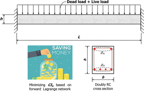
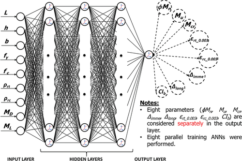
AI-based forward networks implementing Lagrange optimization are formulated based on parameters shown in Table 1(a) that presents forward design scenario, showing nine forward input parameters (L, h, b, f_y,f^’_c, ρ_rt,ρ_rc,M_D,M_L) and eight forward output parameters (ϕM_n,M_u,M_cr,ε_{rt_0.003},ε_{rc_0.003},Δ_imme,Δ_long,CI_b). These parameters include material properties and geometries, which are predetermined by equality constraints. Table 1(b) lists all input and output parameters with their nomenclatures. Forward Lagrange networks are formulated to avoid input conflicts. Conventional software calculates eight output parameters (ϕM_n,M_u,M_cr,ε_{rt_0.003},ε_{rc_0.003},Δ_imme,Δ_long,CI_b) for nine given forward input parameters (L, h, b, f_y,f^’_c, ρ_rt,ρ_rc,M_D,M_L) for a design of ductile doubly reinforced concrete beams. In accordance with ACI 319–14, section 9.3.3.1, tensile rebar strain (ε_{rt_0.003}) should be at least 0.004 to mitigate brittle flexural behavior of RC beam. This limit for tensile rebar strain is denoted as equality $v_9$ in Table 2. In this study, Lagrange optimization technique is implemented to design doubly reinforced RC beams with minimized cost index (CI_b) (refer to Figure 1). The fixed-fixed doubly reinforced concrete (RC) beams were taken into consideration in this study. Immediate deflections were calculated when only live load is taken into consideration in accordance with Table 24.2.2, ACI 318–14 Standard (2014). Cost index of beams (CI_b) was optimized using AI-based Lagrange multiplier method. Besides that, design charts were proposed to assist engineers to design a ductile fixed-fixed doubly RC beam, identifying a minimized CI_b in the preliminary design stage. Cost index of beams (CI_b) is an objective function as a function of nine forward input parameters (L, h, b, f_y,f^’_c, ρ_rt,ρ_rc,M_D, and M_L). In Table 2, six equalities and 11 inequalities are also established for formulating forward Lagrange-based optimization and constructing design charts. Factored moment M_u considering moment due to dead and live load (M_u of 1.2M_D+1.6M_L) is set as equality constraint varying from 500 to 3000 kN·m. Self-weight was subtracted from factored moments because size of the beam is not known in the beginning of a design. Forward Lagrange-based design charts constructed based on minimized cost index of beams (CI_b) are functions of factored moment M_u. The fixed support conditions were reflected in the calculation of the factored moment (M_u), including moment due to dead and live loads as indicated as Equation (1)(1) $M_u=1.2M_D+1.6M_L$(1) .

(1) $M_u=1.2M_D+1.6M_L$(1)

Table 1. Beam design scenario and nomenclature.

(a) Forward design scenario
Forward inputs (nine parameters)
L		h		b			fy		f^’c		$\rho$ rt		$\rho$ rc		MD		ML
Forward outputs (eight parameters)
ϕMn			Mu			Mcr		εrt_0.003		εrc_0.003		Δimme		Δlong		CIb
(b) Nomenclature
No.	Nomenclature
	Forward input parameters
1	L (mm)				Beam span
2	h (mm)				Beam height
3	b (mm)				Beam width
4	fy (MPa)				Yield strength of rebar
5	f^’c (MPa)				Compressive concrete strength
6	ρrt				Tensile rebar ratio of Art to bh; Art is tensile rebar area
7	ρrc				Compressive rebar ratio of Arc to bh; Arc is compressive rebar area
8	MD (kN·m)				Moment due to dead load
9	ML (kN·m)				Moment due to live load
	Forward output parameters
10	ϕMn (kN·m)				Design moment strength excluding moment due to self-weight
11	Mu (kN·m)				Factored moment considering moment due to dead and live load
12	Mcr (kN·m)				Cracking moment
13	εrt_0.003				Tensile rebar strain at concrete strain of 0.003
14	εrc_0.003				Compressive rebar strain at concrete strain of 0.003
15	Δimme				Immediate deflections due to live load
16	Δlong				Long-term deflections
17	CIb (KRW/m)				Cost index of beam

Table 2. Six equalities and 11 inequalities defined as artificial neural genes.

EQUALITY CONSTRAINTS	INEQUALITY CONSTRAINTS
$c_1\left(\mathbf{x}\right):L=10000\mathrm{m}\mathrm{m}$	$v_1\left(\mathbf{x}\right):\varphi M_n-M_u\ge 0$
$c_2\left(\mathbf{x}\right):{f_c}^{\prime }=30\mathrm{M}\mathrm{P}\mathrm{a}$	$v_2\left(\mathbf{x}\right):\varphi M_n-1.2M_{cr}\ge 0$
$c_3\left(\mathbf{x}\right):f_y=600\mathrm{M}\mathrm{P}\mathrm{a}$	$v_3\left(\mathbf{x}\right):h-500\ge 0$
$c_4\left(\mathbf{x}\right):M_D=\left[250\tilde{1}500\right]\mathrm{k}\mathrm{N}\cdot \mathrm{m}$	$v_4\left(\mathbf{x}\right):-h+1200\ge 0$
$c_5\left(\mathbf{x}\right):M_L=\left[125\tilde{7}50\right]\mathrm{k}\mathrm{N}\cdot \mathrm{m}$	$v_5\left(\mathbf{x}\right):b-0.3h\ge 0$
$c_6\left(\mathbf{x}\right):M_u=1.2M_D+1.6M_L=\left[500\tilde{3}000\mathrm{k}\mathrm{N}\cdot \mathrm{m}\right]$	$v_6\left(\mathbf{x}\right):-b+0.8h\ge 0$
	$v_7\left(\mathbf{x}\right):-{\rho }_{rc}+{\rho }_{rt}/2\ge 0$
	$v_8\left(\mathbf{x}\right):{\rho }_{rc}-{\rho }_{rt}/400\ge 0$
	$v_9\left(\mathbf{x}\right):{\epsilon }_{rt\mathrm{\_}0.003}-0.004\ge 0$
	$v_{10}\left(\mathbf{x}\right):-{\mathrm{\Delta }}_{imme}+L/360\ge 0$
	$v_{11}\left(\mathbf{x}\right):-{\mathrm{\Delta }}_{long}+L/240\ge 0$

Figure 1. A doubly reinforced concrete beam with fixed-fixed boundary conditions; cost (CI_b) optimized based on AI-based forward Lagrange network.

Cost index of beams (CI_b, an objective function of the design) is minimized by inequality constraints including a rebar strain (ε_rt). Design parameters including h, b, ${\rho }_{rt}$, and ${\rho }_{rc}$ corresponding to minimum CI_b (cost index) are identified for a given factored moment M_u. The least cost index of beams (CI_b) is determined based on the AI-based Lagrange multiplier method by finding saddle points with convex or concave points of an objective function within the inequality constraints shown in Table 2.

2.2. Formulation of optimization for designs

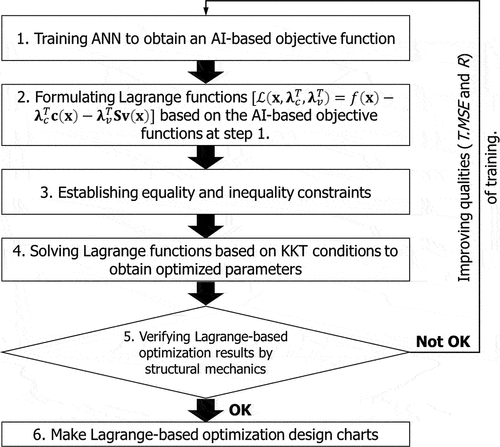
Lagrange optimization technique is implemented in a design of doubly reinforced concrete beams. Cost index (CI_b) was optimized for an RC beam using Lagrange multiplier method. AI-based forward networks implementing Lagrange optimization are formulated based on these parameters. The design algorithm optimizes an objective function based on forward networks shown in Figure 2 where six steps are presented to formulate an AI-based Lagrange multiplier function.

Figure 2. Algorithm for neural network for optimized designs of a ductile precast beam.

2.2.1. Derivation of AI-based objective function and Lagrange function

In this study, a universal approximation function is extracted for objective functions by using ANN as shown in Equation (2)(2) $f\left(\mathbf{x}\right)=g^D\left(f_{lin}^N\left({\mathbf{W}}^N{f}_t^{N-1}\left({\mathbf{W}}^{N-1}\dots f_t^1\left({\mathbf{W}}^1{g}^N\left(\mathbf{x}\right)+{\mathbf{b}}^1\right)\dots +{\mathbf{b}}^{N-1}\right)+b^N\right)\right)$(2) . Krenker, Bešter, and Kos (2011)

(2) $f\left(\mathbf{x}\right)=g^D\left(f_{lin}^N\left({\mathbf{W}}^N{f}_t^{N-1}\left({\mathbf{W}}^{N-1}\dots f_t^1\left({\mathbf{W}}^1{g}^N\left(\mathbf{x}\right)+{\mathbf{b}}^1\right)\dots +{\mathbf{b}}^{N-1}\right)+b^N\right)\right)$(2)

where $\mathbf{x}$ is an input vector; $N$ is a number of layers including hidden layers and output layer; ${\mathbf{W}}^n$ is the weight matrix between layer $n-1$ and layer $n$; ${\mathbf{b}}^n$ is the bias matrix of layer $n$; and $g^N$, $g^D$ are normalization and de-normalization function, respectively. Activation functions $f_t^n$ at layer $n$, were implemented to formulate non-linear relationships of the networks, whereas a linear activation function, $f_{lin}^n$, was selected for output layer because output values are unbounded. Then, an AI-based objective function is used for Lagrange optimization.

Type of networks implementing Lagrange formulation is determined depending on design natures. Reverse network-based Lagrange formulation may be selected when input conflicts can be obviously avoided. Otherwise, forward neural networks should be employed with the aim of removing input conflicts. An AI-based objective function is defined with nine input parameters (L, h, b, f_y,f^’_c, ρ_rt,ρ_rc,M_D,M_L) as shown in Equation (3)(3) $\underset{[1\times 1]}{\underbrace{C{I}_b}}=g_{C{I}_b}^D\left(f_l^3\left(\underset{[1\times 50]}{\underbrace{{\mathbf{W}}_{C{I}_c}^3}}{f}_t^2\left(\underset{[50\times 50]}{\underbrace{{\mathbf{W}}_{C{I}_c}^2}}\dots f_t^1\left(\underset{[50\times 9]}{\underbrace{{\mathbf{W}}_{C{I}_c}^1}}\underset{[9\times 1]}{\underbrace{g_{C{I}_c}^N\left(\mathbf{x}\right)}}+\underset{[50\times 1]}{\underbrace{{\mathbf{b}}_{C{I}_c}^1}}\right)\dots +\underset{[50\times 1]}{\underbrace{{\mathbf{b}}_{C{I}_c}^2}}\right)+\underset{[1\times 1]}{\underbrace{b_{C{I}_c}^3}}\right)\right)$(3) to optimize cost index (CI_b) of a doubly RC beam. Boundary conditions of beams are predetermined by engineers before generating big datasets. In this study, the authors assume fixed boundary conditions of beams. Therefore, big datasets and structural calculation software are made based on the fixed-fixed beams. Output parameters that are influenced mostly by beam length (L) are immediate (Δ_imme) and long-term (Δ_long) deflections. Immediate (Δ_imme) and long-term (Δ_long) deflections were constrained not to be greater than L/360 and L/240 (Table 24.2.2, ACI 318–14 Standard (2014)), respectively, as indicated as inequality constraints ($v_{10}$ and $v_{11}$ in Table 2).

The best training ANN on cost index (CI_b) with three layers and 50 neurons was presented in Table 3.

(3) $\underset{[1\times 1]}{\underbrace{C{I}_b}}=g_{C{I}_b}^D\left(f_l^3\left(\underset{[1\times 50]}{\underbrace{{\mathbf{W}}_{C{I}_c}^3}}{f}_t^2\left(\underset{[50\times 50]}{\underbrace{{\mathbf{W}}_{C{I}_c}^2}}\dots f_t^1\left(\underset{[50\times 9]}{\underbrace{{\mathbf{W}}_{C{I}_c}^1}}\underset{[9\times 1]}{\underbrace{g_{C{I}_c}^N\left(\mathbf{x}\right)}}+\underset{[50\times 1]}{\underbrace{{\mathbf{b}}_{C{I}_c}^1}}\right)\dots +\underset{[50\times 1]}{\underbrace{{\mathbf{b}}_{C{I}_c}^2}}\right)+\underset{[1\times 1]}{\underbrace{b_{C{I}_c}^3}}\right)\right)$(3)

Table 3. Summary of training results.

(a) Network 1
(1) 9 Inputs (L, h, b, fy,f^’c, ρrt,ρrc,MD,ML) – 1 Output (ϕMn)
Datasets	Layers	Neurons	Required Epoch	Best Epoch for Training	Test MSE		R at Best Epoch
100,000	3	30	50,000	19,875	1.83E-06		1.0
(2) 9 Inputs (L, h, b, fy,f^’c, ρrt,ρrc,MD,ML) – 1 Output (Mu)
Data	Layers	Neurons	Required Epoch	Best Epoch for Training	Test MSE		R at Best Epoch
100,000	3	30	50,000	11,812	4.64E-08		1.0
(3) 9 Inputs (L, h, b, fy,f^’c, ρrt,ρrc,MD,ML) – 1 Output (Mcr)
Data	Layers	Neurons	Required Epoch	Best Epoch for Training	Test MSE		R at Best Epoch
100,000	3	40	50,000	14,305	9.60E-07		1.0
(4) 9 Inputs (L, h, b, fy,f^’c, ρrt,ρrc,MD,ML) – 1 Output (εrt_0.003)
Data	Layers	Neurons	Required Epoch	Best Epoch for Training	Test MSE		R at Best Epoch
100,000	3	50	50,000	14,305	3.03E-06		1.0
(5) 9 Inputs (L, h, b, fy,f^’c, ρrt,ρrc,MD,ML) – 1 Output (εrc_0.003)
Data	Layers	Neurons	Required Epoch	Best Epoch for Training	Test MSE		R at Best Epoch
100,000	3	30	50,000	18,387	6.44E-06		1.0
(6) 9 Inputs (L, h, b, fy,f^’c, ρrt,ρrc,MD,ML) – 1 Output (Δimme)
Data	Layers	Neurons	Required Epoch	Best Epoch for Training	Test MSE		R at Best Epoch
100,000	3	40	50,000	20,710	1.63E-04		0.998
(7) 9 Inputs (L, h, b, fy,f^’c, ρrt,ρrc,MD,ML) – 1 Output (Δlong)
Data	Layers	Neurons	Required Epoch	Best Epoch for Training	Test MSE		R at Best Epoch
100,000	3	40	50,000	25,404	5.89E-05		1.000
(8) 9 Inputs (L, h, b, fy,f^’c, ρrt,ρrc,MD,ML) – 1 Output (CIb)
Data	Layers	Neurons	Required Epoch	Best Epoch for Training	Test MSE		R at Best Epoch
100,000	3	50	50,000	23,775	7.31E-08		1.0
(b) Network 2
(1) 9 Inputs (L, h, b, fy,f^’c, ρrt,ρrc,MD,ML) – 1 Output (ϕMn)
Datasets	Layers	Neurons	Required Epoch	Best Epoch for Training		Test MSE		R at Best Epoch
100,000	3	30	50,000	19,875		1.83E-06		1.0
(2) 9 Inputs (L, h, b, fy,f^’c, ρrt,ρrc,MD,ML) – 1 Output (Mu)
Data	Layers	Neurons	Required Epoch	Best Epoch for Training		Test MSE		R at Best Epoch
100,000	3	30	50,000	11,812		4.64E-08		1.0
(3) 9 Inputs (L, h, b, fy,f^’c, ρrt,ρrc,MD,ML) – 1 Output (Mcr)
Data	Layers	Neurons	Required Epoch	Best Epoch for Training		Test MSE		R at Best Epoch
100,000	3	40	50,000	14,305		9.60E-07		1.0
(4) 9 Inputs (L, h, b, fy,f^’c, ρrt,ρrc,MD,ML) – 1 Output (εrt_0.003)
Data	Layers	Neurons	Required Epoch	Best Epoch for Training		Test MSE		R at Best Epoch
100,000	3	50	50,000	14,305		3.03E-06		1.0
(5) 9 Inputs (L, h, b, fy,f^’c, ρrt,ρrc,MD,ML) – 1 Output (εrc_0.003)
Data	Layers	Neurons	Required Epoch	Best Epoch for Training		Test MSE		R at Best Epoch
100,000	3	30	50,000	18,387		6.44E-06		1.0
(6) 9 Inputs (L, h, b, fy,f^’c, ρrt,ρrc,MD,ML) – 1 Output (Δimme)
Data	Layers	Neurons	Required Epoch	Best Epoch for Training		Test MSE		R at Best Epoch
100,000	4	40	50,000	27,771		1.47E-04		0.999
(7) 9 Inputs (L, h, b, fy,f^’c, ρrt,ρrc,MD,ML) – 1 Output (Δlong)
Data	Layers	Neurons	Required Epoch	Best Epoch for Training		Test MSE		R at Best Epoch
100,000	5	20	50,000	37,451		5.64E-05		1.000
(8) 9 Inputs (L, h, b, fy,f^’c, ρrt,ρrc,MD,ML) – 1 Output (CIb)
Data	Layers	Neurons	Required Epoch	Best Epoch for Training		Test MSE		R at Best Epoch
100,000	3	50	50,000	23,775		7.31E-08		1.0

A Lagrange function, $\mathcal{L}$, is considered as a function of variables $\mathbf{x}={\left[x_1,x_2,\dots ,x_n\right]}^T$, equality ($\mathbf{c}\left(\mathbf{x}\right)$) and inequality ($\mathbf{v}\left(\mathbf{x}\right)$) constraints, and Lagrange multiplier of equality constraints and inequality constraints, ${\lambda }_c={\left[{\lambda }_1,{\lambda }_2,\dots ,{\lambda }_m\right]}^T$ and ${\lambda }_v={\left[{\lambda }_1,{\lambda }_2,\dots ,{\lambda }_l\right]}^T$, respectively, as shown in Equation (4)(4) $\mathcal{L}\left(\mathbf{x},{\lambda }_c^T,{\lambda }_v^T\right)=f\left(\mathbf{x}\right)-{\lambda }_c^T\mathbf{c}\left(\mathbf{x}\right)-{\lambda }_v^T\mathbf{S}\mathbf{v}\left(\mathbf{x}\right)=C{I}_b-{\lambda }_c^T\mathbf{c}\left(\mathbf{x}\right)-{\lambda }_v^T\mathbf{S}\mathbf{v}\left(\mathbf{x}\right)$(4) :

(4) $\mathcal{L}\left(\mathbf{x},{\lambda }_c^T,{\lambda }_v^T\right)=f\left(\mathbf{x}\right)-{\lambda }_c^T\mathbf{c}\left(\mathbf{x}\right)-{\lambda }_v^T\mathbf{S}\mathbf{v}\left(\mathbf{x}\right)=C{I}_b-{\lambda }_c^T\mathbf{c}\left(\mathbf{x}\right)-{\lambda }_v^T\mathbf{S}\mathbf{v}\left(\mathbf{x}\right)$(4)

As shown in Table 2, six simple equalities including L, f_y,f^’_c, M_D,M_L and M_u can be substituted directly in networks. Eleven inequality constraints are shown in Table 2 to constraint optimization process. Equalities are equations, not variables, and, hence they must be written as f_y = 600 or f_y $-600$ = 0.

Newton-Raphson technique is applied to solve a set of partial differential equations, $\mathrm{\nabla }\mathcal{L}\left(\mathbf{x},{\lambda }_c,{\lambda }_v\right)$, which is, then, needed to be differentiated once in order to find stationary points of Lagrange function, $\mathcal{L}\left(\mathbf{x},{\lambda }_c,{\lambda }_v\right)$ with respect to a function of variables, x, Lagrange multiplier of equality constraints, ${\lambda }_c$, and Lagrange multiplier of inequality constraints, ${\lambda }_v$. A procedure to solve $\mathrm{\nabla }\mathcal{L}\left(\mathbf{x},{\lambda }_c,{\lambda }_v\right)$ to find saddle points of Lagrange functions using Newton-Raphson technique based on Jacobian and Hessian matrix is shown in Equations (5(5) $\left[\begin{array}{c}{\mathbf{x}}^{\left(\mathrm{k}+1\right)}\\ {\lambda }_c^{\left(k+1\right)}\\ {\lambda }_v^{\left(k+1\right)}\end{array}\right]=\left[\begin{array}{c}{\mathbf{x}}^{\left(\mathrm{k}\right)}\\ {\lambda }_c^{\left(k\right)}\\ {\lambda }_v^{\left(k\right)}\end{array}\right]-{\left[H_{\mathcal{L}}\left({\mathbf{x}}^{\left(\mathrm{k}\right)},{\lambda }_c^{\left(\mathrm{k}\right)},{\lambda }_v^{\left(\mathrm{k}\right)}\right)\right]}^{-1}\mathrm{\nabla }\mathcal{L}\left({\mathbf{x}}^{\left(\mathrm{k}\right)},{\lambda }_c^{\left(\mathrm{k}\right)},{\lambda }_v^{\left(\mathrm{k}\right)}\right)$(5) –7(7) $J_{\mathbf{c}}\left(\mathbf{x}\right)=\left[\begin{array}{c}\mathrm{\nabla }{c}_1\left(\mathbf{x}\right)\\ \mathrm{\nabla }{c}_2\left(\mathbf{x}\right)\\ ⋮\\ \mathrm{\nabla }{c}_m\left(\mathbf{x}\right)\end{array}\right]\mathrm{a}\mathrm{n}\mathrm{d}{J}_{\mathbf{v}}\left(\mathbf{x}\right)=\left[\begin{array}{c}\mathrm{\nabla }{v}_1\left(\mathbf{x}\right)\\ \mathrm{\nabla }{v}_2\left(\mathbf{x}\right)\\ ⋮\\ \mathrm{\nabla }{v}_l\left(\mathbf{x}\right)\end{array}\right]$(7) ). The variable $\mathbf{x}$ and Lagrange multipliers $\lambda$ can be updated after every iteration based on Newton–Raphson technique as indicated in Equation (5)(5) $\left[\begin{array}{c}{\mathbf{x}}^{\left(\mathrm{k}+1\right)}\\ {\lambda }_c^{\left(k+1\right)}\\ {\lambda }_v^{\left(k+1\right)}\end{array}\right]=\left[\begin{array}{c}{\mathbf{x}}^{\left(\mathrm{k}\right)}\\ {\lambda }_c^{\left(k\right)}\\ {\lambda }_v^{\left(k\right)}\end{array}\right]-{\left[H_{\mathcal{L}}\left({\mathbf{x}}^{\left(\mathrm{k}\right)},{\lambda }_c^{\left(\mathrm{k}\right)},{\lambda }_v^{\left(\mathrm{k}\right)}\right)\right]}^{-1}\mathrm{\nabla }\mathcal{L}\left({\mathbf{x}}^{\left(\mathrm{k}\right)},{\lambda }_c^{\left(\mathrm{k}\right)},{\lambda }_v^{\left(\mathrm{k}\right)}\right)$(5) . The procedure for Newton–Raphson approximation is repeated until convergence is achieved.

(5) $\left[\begin{array}{c}{\mathbf{x}}^{\left(\mathrm{k}+1\right)}\\ {\lambda }_c^{\left(k+1\right)}\\ {\lambda }_v^{\left(k+1\right)}\end{array}\right]=\left[\begin{array}{c}{\mathbf{x}}^{\left(\mathrm{k}\right)}\\ {\lambda }_c^{\left(k\right)}\\ {\lambda }_v^{\left(k\right)}\end{array}\right]-{\left[H_{\mathcal{L}}\left({\mathbf{x}}^{\left(\mathrm{k}\right)},{\lambda }_c^{\left(\mathrm{k}\right)},{\lambda }_v^{\left(\mathrm{k}\right)}\right)\right]}^{-1}\mathrm{\nabla }\mathcal{L}\left({\mathbf{x}}^{\left(\mathrm{k}\right)},{\lambda }_c^{\left(\mathrm{k}\right)},{\lambda }_v^{\left(\mathrm{k}\right)}\right)$(5)

where $\left[H_{\mathcal{L}}\left({\mathbf{x}}^{\left(\mathrm{k}\right)},{\lambda }_c^{\left(\mathrm{k}\right)},{\lambda }_v^{\left(\mathrm{k}\right)}\right)\right]$ is Hessian matrix of Lagrange function; $\mathrm{\nabla }\mathcal{L}\left({\mathbf{x}}^{\left(\mathrm{k}\right)},{\lambda }_c^{\left(\mathrm{k}\right)},{\lambda }_v^{\left(\mathrm{k}\right)}\right)$ is the first derivation of Lagrange function based on KKT conditions in order to find slopes of the parallel tangential lines of the objective functions considering equality $\mathbf{c}\left(\mathbf{x}\right)$ and inequality $\mathbf{v}\left(\mathbf{x}\right)$ constraints.

(6) $\mathrm{\nabla }\mathcal{L}\left(\mathbf{x},{\lambda }_c,{\lambda }_v\right)=\left[\begin{array}{c}\begin{array}{c}\mathrm{\nabla }f\left(\mathbf{x}\right)-J_{\mathbf{c}}{\left(\mathbf{x}\right)}^T{\lambda }_c-J_{\mathbf{v}}{\left(\mathbf{x}\right)}^T\mathbf{S}{\lambda }_v\\ -\mathbf{c}\left(\mathbf{x}\right)\end{array}\\ -\mathbf{S}\mathbf{v}\left(\mathbf{x}\right)\end{array}\right]$(6)

(7) $J_{\mathbf{c}}\left(\mathbf{x}\right)=\left[\begin{array}{c}\mathrm{\nabla }{c}_1\left(\mathbf{x}\right)\\ \mathrm{\nabla }{c}_2\left(\mathbf{x}\right)\\ ⋮\\ \mathrm{\nabla }{c}_m\left(\mathbf{x}\right)\end{array}\right]\mathrm{a}\mathrm{n}\mathrm{d}{J}_{\mathbf{v}}\left(\mathbf{x}\right)=\left[\begin{array}{c}\mathrm{\nabla }{v}_1\left(\mathbf{x}\right)\\ \mathrm{\nabla }{v}_2\left(\mathbf{x}\right)\\ ⋮\\ \mathrm{\nabla }{v}_l\left(\mathbf{x}\right)\end{array}\right]$(7)

In which $J_{\mathbf{c}}\left(\mathbf{x}\right)$ and $J_{\mathbf{v}}\left(\mathbf{x}\right)$ are Jacobian matrix of constraint vectors $\mathbf{c}$ and $\mathbf{v}$, at $\mathbf{x}$, respectively. The Lagrange multipliers for both equality (${\lambda }_c$) and inequality (${\lambda }_v$) constraints are implemented to convert constrained optimization problems to unconstrained ones.

2.2.2. Formulation of equality and inequality constraints to generate active, inactive constraint combinations

Equality constraint vector is given in Equation (8)(8) $c\left(x\right)={\left[c_1\left(x\right),c_2\left(x\right),\dots ,c_6\left(x\right)\right]}^T$(8) and Table 2 with Lagrange multipliers of equality constraints shown as ${\lambda }_c={\left[{\lambda }_{c1},{\lambda }_{c2},\dots ,{\lambda }_{c6}\right]}^T$. Inequality constraint vector is also given in Equation (9)(9) $v\left(x\right)={\left[v_1\left(x\right),v_2\left(x\right),\dots ,v_{11}\left(x\right)\right]}^T$(9) and Table 2 with Lagrange multipliers of inequality constraints shown as constraints shown as ${\lambda }_v={\left[{\lambda }_{v1},{\lambda }_{v2},\dots ,{\lambda }_{v11}\right]}^T$.

(8) $c\left(x\right)={\left[c_1\left(x\right),c_2\left(x\right),\dots ,c_6\left(x\right)\right]}^T$(8)

(9) $v\left(x\right)={\left[v_1\left(x\right),v_2\left(x\right),\dots ,v_{11}\left(x\right)\right]}^T$(9)

Inequality matrix $\mathbf{S}$ (matrix for inequality constraints) is introduced to identify active inequality constraints as shown in Equation (10)(10) $\mathbf{S}={\left[\begin{array}{cccc}{s}_1& 0& \cdots & 0\\ 0& s_2& \cdots & 0\\ ⋮& ⋮& \ddots & ⋮\\ 0& 0& \cdots & s_{11}\end{array}\right]}_{\left[11\times 11\right]}$(10) where active inequality constraints ($v_i$) are shown.

(10) $\mathbf{S}={\left[\begin{array}{cccc}{s}_1& 0& \cdots & 0\\ 0& s_2& \cdots & 0\\ ⋮& ⋮& \ddots & ⋮\\ 0& 0& \cdots & s_{11}\end{array}\right]}_{\left[11\times 11\right]}$(10)

2.2.2.1. Formulation of inequality matrix

In Equation (10)(10) $\mathbf{S}={\left[\begin{array}{cccc}{s}_1& 0& \cdots & 0\\ 0& s_2& \cdots & 0\\ ⋮& ⋮& \ddots & ⋮\\ 0& 0& \cdots & s_{11}\end{array}\right]}_{\left[11\times 11\right]}$(10) , inequality matrix $\mathbf{S}$ is obtained in which inequality constraints ($v_i$) are activated by $s_i$. Inequality constraints ($v_i$) are activated when $s_i=1$ while inequality constraints ($v_i$) are not activated when $s_i=0$.

The code requirements are expressed in term of inequality constraints; $v_2=\varphi M_n-1.2M_{cr}\ge 0$ which is constrained by ACI 318–14 (Section 9.6.1.2) Standard (2014) in which the minimum limit of tensile rebar ratio is controlled as shown in inequality constraint, $v_2$, of Table 2.

Inequality constraint ($v_2$) is activated when $s_2=$ 1 with design moment strength $\varphi M_n$ being 1.2 times cracking moment M_cr, leading to Equation (11)(11) $S={\left[\begin{array}{ccccccc}{1}^{st}& 2^{nd}& 3^{rd}& \cdots & {10}^{th}& {11}^{th}& \\ s_1=0& 0& 0& \cdots & 0& 0& 1^{st}\\ 0& s_2=1& 0& \cdots & 0& 0& 2^{nd}\\ ⋮& ⋮& ⋮& \ddots & ⋮& ⋮& ⋮\\ 0& 0& 0& \cdots & 0& 0& 9^{th}\\ 0& 0& 0& \cdots & s_{10}=0& 0& {10}^{th}\\ 0& 0& 0& \cdots & 0& s_{11}=0& {11}^{th}\end{array}\right]}_{\left[11\times 11\right]}$(11) .

(11) $S={\left[\begin{array}{ccccccc}{1}^{st}& 2^{nd}& 3^{rd}& \cdots & {10}^{th}& {11}^{th}& \\ s_1=0& 0& 0& \cdots & 0& 0& 1^{st}\\ 0& s_2=1& 0& \cdots & 0& 0& 2^{nd}\\ ⋮& ⋮& ⋮& \ddots & ⋮& ⋮& ⋮\\ 0& 0& 0& \cdots & 0& 0& 9^{th}\\ 0& 0& 0& \cdots & s_{10}=0& 0& {10}^{th}\\ 0& 0& 0& \cdots & 0& s_{11}=0& {11}^{th}\end{array}\right]}_{\left[11\times 11\right]}$(11)

Lagrange optimization function with $s_2=$ 1 is obtained in Equation (12)(12) ${\mathcal{L}}_{C{I}_b}\left(\mathbf{x},{\lambda }_c,{\lambda }_v\right)=C{I}_b-{\lambda }_c^T\mathbf{c}\left(\mathbf{x}\right)-{\lambda }_v^T{\left[\begin{array}{cccc}{s}_1=0& 0& \cdots & 0\\ 0& s_2=1& \cdots & 0\\ ⋮& ⋮& \ddots & ⋮\\ 0& 0& \cdots & s_{11}=0\end{array}\right]}_{\left[11\times 11\right]}\mathbf{v}\left(\mathbf{x}\right)$(12) by substituting ${\mathrm{s}}_2$ of 1 [Equation (11)(11) $S={\left[\begin{array}{ccccccc}{1}^{st}& 2^{nd}& 3^{rd}& \cdots & {10}^{th}& {11}^{th}& \\ s_1=0& 0& 0& \cdots & 0& 0& 1^{st}\\ 0& s_2=1& 0& \cdots & 0& 0& 2^{nd}\\ ⋮& ⋮& ⋮& \ddots & ⋮& ⋮& ⋮\\ 0& 0& 0& \cdots & 0& 0& 9^{th}\\ 0& 0& 0& \cdots & s_{10}=0& 0& {10}^{th}\\ 0& 0& 0& \cdots & 0& s_{11}=0& {11}^{th}\end{array}\right]}_{\left[11\times 11\right]}$(11) ] into Equation (4)(4) $\mathcal{L}\left(\mathbf{x},{\lambda }_c^T,{\lambda }_v^T\right)=f\left(\mathbf{x}\right)-{\lambda }_c^T\mathbf{c}\left(\mathbf{x}\right)-{\lambda }_v^T\mathbf{S}\mathbf{v}\left(\mathbf{x}\right)=C{I}_b-{\lambda }_c^T\mathbf{c}\left(\mathbf{x}\right)-{\lambda }_v^T\mathbf{S}\mathbf{v}\left(\mathbf{x}\right)$(4) .

(12) ${\mathcal{L}}_{C{I}_b}\left(\mathbf{x},{\lambda }_c,{\lambda }_v\right)=C{I}_b-{\lambda }_c^T\mathbf{c}\left(\mathbf{x}\right)-{\lambda }_v^T{\left[\begin{array}{cccc}{s}_1=0& 0& \cdots & 0\\ 0& s_2=1& \cdots & 0\\ ⋮& ⋮& \ddots & ⋮\\ 0& 0& \cdots & s_{11}=0\end{array}\right]}_{\left[11\times 11\right]}\mathbf{v}\left(\mathbf{x}\right)$(12)

where ${\lambda }_c\mathrm{a}\mathrm{n}\mathrm{d}\hspace{0.17em}{\lambda }_v$ are Lagrange multipliers with respect to $c_i\left(\mathbf{x}\right)$ and $v_j\left(\mathbf{x}\right),$ respectively.

The maximum limit of tensile rebar ratio is controlled by a minimum tensile rebar strain of 0.004, which is represented by inequality $v_9$ of Table 2. Then, inequality matrix $\mathbf{S}$ becomes Equation (13)(13) $S={\left[\begin{array}{cccccccc}{1}^{st}& 2^{nd}& 3^{rd}& \cdots & 9^{th}& {10}^{th}& {11}^{th}& \hspace{0.17em}\\ s_1=0& 0& 0& \cdots & 0& 0& 0& 1^{st}\\ 0& s_2=0& 0& \cdots & 0& 0& 0& 2^{nd}\\ 0& 0& s_3=0& \cdots & 0& 0& 0& 3^{rd}\\ ⋮& ⋮& ⋮& \ddots & \cdots & ⋮& ⋮& ⋮\\ 0& 0& 0& \cdots & s_9=0& 0& 0& ⋮\\ 0& 0& 0& \cdots & 0& s_{10}=0& 0& {10}^{th}\\ 0& 0& 0& \cdots & 0& 0& s_{11}=0& {11}^{th}\end{array}\right]}_{[11\times 11]}$(13) where inequality constraint ($v_9$) is activated when $s_9=$ 1.

(13) $S={\left[\begin{array}{cccccccc}{1}^{st}& 2^{nd}& 3^{rd}& \cdots & 9^{th}& {10}^{th}& {11}^{th}& \hspace{0.17em}\\ s_1=0& 0& 0& \cdots & 0& 0& 0& 1^{st}\\ 0& s_2=0& 0& \cdots & 0& 0& 0& 2^{nd}\\ 0& 0& s_3=0& \cdots & 0& 0& 0& 3^{rd}\\ ⋮& ⋮& ⋮& \ddots & \cdots & ⋮& ⋮& ⋮\\ 0& 0& 0& \cdots & s_9=0& 0& 0& ⋮\\ 0& 0& 0& \cdots & 0& s_{10}=0& 0& {10}^{th}\\ 0& 0& 0& \cdots & 0& 0& s_{11}=0& {11}^{th}\end{array}\right]}_{[11\times 11]}$(13)

Lagrange optimization function with $s_9=$ 1 is obtained in Equation (14)(14) ${\mathcal{L}}_{C{I}_b}\left(\mathbf{x},{\lambda }_c,{\lambda }_v\right)=C{I}_b-{\lambda }_c^T\mathbf{c}\left(\mathbf{x}\right)-{\lambda }_v^T{\left[\begin{array}{ccccccc}{s}_1=0& 0& \cdots & \cdots & \cdots & 0& 0\\ 0& s_2=0& \cdots & \cdots & \cdots & 0& 0\\ 0& 0& \ddots & \cdots & \cdots & 0& 0\\ ⋮& ⋮& ⋮& \ddots & ⋮& ⋮& ⋮\\ ⋮& ⋮& ⋮& ⋮& s_9=1& ⋮& ⋮\\ 0& 0& \cdots & \cdots & \cdots & s_{10}=0& 0\\ 0& 0& \cdots & \cdots & \cdots & 0& s_{11}=0\end{array}\right]}_{\left[11\times 11\right]}\mathbf{v}\left(\mathbf{x}\right)$(14) by substituting $\hspace{0.17em}{\mathrm{s}}_9$ equivalent to 1 into Equation (4)(4) $\mathcal{L}\left(\mathbf{x},{\lambda }_c^T,{\lambda }_v^T\right)=f\left(\mathbf{x}\right)-{\lambda }_c^T\mathbf{c}\left(\mathbf{x}\right)-{\lambda }_v^T\mathbf{S}\mathbf{v}\left(\mathbf{x}\right)=C{I}_b-{\lambda }_c^T\mathbf{c}\left(\mathbf{x}\right)-{\lambda }_v^T\mathbf{S}\mathbf{v}\left(\mathbf{x}\right)$(4) .

(14) ${\mathcal{L}}_{C{I}_b}\left(\mathbf{x},{\lambda }_c,{\lambda }_v\right)=C{I}_b-{\lambda }_c^T\mathbf{c}\left(\mathbf{x}\right)-{\lambda }_v^T{\left[\begin{array}{ccccccc}{s}_1=0& 0& \cdots & \cdots & \cdots & 0& 0\\ 0& s_2=0& \cdots & \cdots & \cdots & 0& 0\\ 0& 0& \ddots & \cdots & \cdots & 0& 0\\ ⋮& ⋮& ⋮& \ddots & ⋮& ⋮& ⋮\\ ⋮& ⋮& ⋮& ⋮& s_9=1& ⋮& ⋮\\ 0& 0& \cdots & \cdots & \cdots & s_{10}=0& 0\\ 0& 0& \cdots & \cdots & \cdots & 0& s_{11}=0\end{array}\right]}_{\left[11\times 11\right]}\mathbf{v}\left(\mathbf{x}\right)$(14)

where ${\lambda }_{\hspace{0.17em}}\mathrm{a}\mathrm{n}\mathrm{d}\hspace{0.17em}{\lambda }_v$ are Lagrange multipliers with respect to $c_i\left(\mathbf{x}\right)$ and $v_j\left(\mathbf{x}\right),$ respectively.

2.2.2.2. None is activated

An inequality constraint is said to be active (or tight, binding), otherwise, they are called inactive or slacked. Lagrange function multipliers should be greater than zero for equality and active inequality constraints while they should be zero values, ignoring inactive inequality constraints when generating Lagrange function and KKT conditions. With KKT conditions (all equality and inequality conditions), Lagrange function with multipliers should be tested for optimality conditions. Lagrange multiplier is going to be strictly positive when the constraint is not slack but active or binding (slack is equal to zero in this case) because essentially imposing the constraints is influencing Lagrange function. When there is a slack (inactive) on the constraint, Lagrange function is not influenced, imposing the inactive constraints that do not cost anything, and hence, Lagrange multipliers (${\lambda }_c$) is equal to zero.

The design example is shown in Equation (15)(15) $\mathbf{S}={\left[\begin{array}{cccc}0& 0& \cdots & 0\\ 0& 0& \cdots & 0\\ ⋮& ⋮& \ddots & ⋮\\ 0& 0& \cdots & 0\end{array}\right]}_{\left[11\times 11\right]}$(15) where none of inequalities is active with s_i being 0.

(15) $\mathbf{S}={\left[\begin{array}{cccc}0& 0& \cdots & 0\\ 0& 0& \cdots & 0\\ ⋮& ⋮& \ddots & ⋮\\ 0& 0& \cdots & 0\end{array}\right]}_{\left[11\times 11\right]}$(15)

Lagrange optimization function with all s_i equal to 0 is obtained in Equation (16)(16) ${\mathcal{L}}_{C{I}_b}\left(\mathbf{x},{\lambda }_c,{\lambda }_v\right)=C{I}_b-{\lambda }_c^T\mathbf{c}\left(\mathbf{x}\right)-{\lambda }_v^T{\left[\begin{array}{cccc}0& 0& \cdots & 0\\ 0& 0& \cdots & 0\\ ⋮& ⋮& \ddots & ⋮\\ 0& 0& \cdots & 0\end{array}\right]}_{\left[11\times 11\right]}\mathbf{v}\left(\mathbf{x}\right)$(16) by substituting Equation (15)(15) $\mathbf{S}={\left[\begin{array}{cccc}0& 0& \cdots & 0\\ 0& 0& \cdots & 0\\ ⋮& ⋮& \ddots & ⋮\\ 0& 0& \cdots & 0\end{array}\right]}_{\left[11\times 11\right]}$(15) into Equation (4)(4) $\mathcal{L}\left(\mathbf{x},{\lambda }_c^T,{\lambda }_v^T\right)=f\left(\mathbf{x}\right)-{\lambda }_c^T\mathbf{c}\left(\mathbf{x}\right)-{\lambda }_v^T\mathbf{S}\mathbf{v}\left(\mathbf{x}\right)=C{I}_b-{\lambda }_c^T\mathbf{c}\left(\mathbf{x}\right)-{\lambda }_v^T\mathbf{S}\mathbf{v}\left(\mathbf{x}\right)$(4) .

(16) ${\mathcal{L}}_{C{I}_b}\left(\mathbf{x},{\lambda }_c,{\lambda }_v\right)=C{I}_b-{\lambda }_c^T\mathbf{c}\left(\mathbf{x}\right)-{\lambda }_v^T{\left[\begin{array}{cccc}0& 0& \cdots & 0\\ 0& 0& \cdots & 0\\ ⋮& ⋮& \ddots & ⋮\\ 0& 0& \cdots & 0\end{array}\right]}_{\left[11\times 11\right]}\mathbf{v}\left(\mathbf{x}\right)$(16)

where ${\lambda }_c\hspace{0.17em}\mathrm{a}\mathrm{n}\mathrm{d}\hspace{0.17em}{\lambda }_v$ are Lagrange multipliers with respect to $c_i\left(\mathbf{x}\right)$ and $v_j\left(\mathbf{x}\right),\mathrm{r}\mathrm{e}\mathrm{s}\mathrm{p}\mathrm{e}\mathrm{c}\mathrm{t}\mathrm{i}\mathrm{v}\mathrm{e}\mathrm{l}\mathrm{y}.$

It is noted that $\mathbf{S}={\left[\begin{array}{cccc}0& 0& \cdots & 0\\ 0& 0& \cdots & 0\\ ⋮& ⋮& \ddots & ⋮\\ 0& 0& \cdots & 0\end{array}\right]}_{\left[11\times 11\right]}$ cannot take place because design moment strength $\varphi M_n$ and tensile rebar strain ${\epsilon }_{rt\mathrm{\_}0.003}$ corresponding to a concrete strain of 0.003 cannot be equivalent to 1.2 times cracking moment (1.2M_cr) and 0.004 at the same time, respectively. Tensile rebar ratio reaches the maximum value when tensile rebar strain is equivalent to 0.004. The minimum rebar ratio is obtained when design moment strength equals to 1.2 times cracking moment ($\varphi M_n=1.2M_{cr}$). Tensile rebar ratio cannot reach the maximum and minimum value at the same time; therefore, Equation (15)(15) $\mathbf{S}={\left[\begin{array}{cccc}0& 0& \cdots & 0\\ 0& 0& \cdots & 0\\ ⋮& ⋮& \ddots & ⋮\\ 0& 0& \cdots & 0\end{array}\right]}_{\left[11\times 11\right]}$(15) cannot take place.

Simple equality and inequality constraint with single input values established as shown in Table 2 are substituted into initial input vector of (L, h, b, f_y,f^’_c, ρ_rt,ρ_rc,M_D,M_L) for first iteration of Newton-Raphson procedure, reducing complexity of the equality constraint vector (C) and the inequality constraint vector (V). Newton-Raphson method heavily relies on a good initial vector.

Output parameter, such as compressive concrete strain ε_rc_0.003, which is not engaged with any of objective functions, equality, and inequality constraints, not appearing in design scenario, are obtained as a result of Lagrange optimization.

3. Generation of large structural datasets

3.1. Input and output parameters generated for large datasets

Nine input and eight output parameters shown in Table 1 were generated for large datasets to design structural systems in general and to design doubly reinforced concrete beams, in particular, nine input parameters including material properties (yield strength of rebar f_y (MPa) and concrete compressive strength f_c (MPa)), beam geometry (height h (mm), and span length L (m), and moment demand due to dead and live loads (kN·m). Output parameters include design moment strength (ϕM_n), factored moment (M_u), cracking moment (M_cr), compressive and tensile trains of rebars (ε_{rt_0.003} and ε_{rc_0.003}), immediate and long-term deflections (Δ_imme and Δ_long), and cost index (CI_b, KRW/m) for materials and manufacture of an RC beam. However, more network inputs and outputs can be adopted depending on a need of an analysis and design.

3.2. Random design ranges

The strain-compatibility-based algorithm (Autobeam) was developed for a design of ductile doubly reinforced concrete beams in the authors’ previous study Nguyen, Hong, and Part (2019). Large structural datasets that were generated based on Autobeam were used to train ANN for design. Table 4 presents a number of datasets, mean values, variances, standard deviation, and ranges of selected network input and output parameters, which were randomly generated for a design of doubly RC beams. Random datasets for rebar yield strengths f_y and for concrete compressive strengths f_c were generated in the range 500–600 MPa and 30–50 MPa, respectively, to consider a wide range of beam designs for beam lengths spanning 8–12 m. Beam height and width were randomized in the range 400–1500 mm and (0.25–0.8)h.

Table 4. List of random variables and corresponding ranges.

	L (mm)	h (mm)	b (mm)	f^’c (MPa)	fy (MPa)	ρrt	ρrc	MD (kN·m)	ML (kN·m)
Number of datasets	100,000
Maximum	12,000	1500	1200	50	600	0.05	0.025	22,159	10,783
Mean	10,000	951	520	40	550	0.015	0.004	1766	542
Minimum	8000	400	120	30	500	0.0023	8.92E-06	3	0
Variance (V)	1,366,497	101,574	52,002	37	849	9.21E-05	1.73E-05	5,288,086	687,577
Standard deviation	1168	318	228	6	29	9.59E-03	4.16E-03	2300	829

3.3. Network training based on Parallel Training Method (PTM) training

In this study, input vector is mapped to each output parameter by using parallel training method (PTM). A PTM method separates outputs to groups to train them in parallel. Less time for training is required for this method than mapping input vector to all output parameters, however, feature indexes appeared in the same network output still cannot be used as input feature indexes to predict other outputs. In this study, the forward network was trained using PTM training method on nine input parameters (L, h, b, f_y,f^’_c, ρ_rt,ρ_rc,M_D,M_L) and eight outputs (ϕM_n,M_u,M_cr,Δ_imme,Δ_long,ε_{rt_0.003},ε_{rc_0.003},CI_b) as illustrated in Figure 3.

Figure 3. Topology of forward network using PTM training method.

3.4. Training for forward Lagrange networks

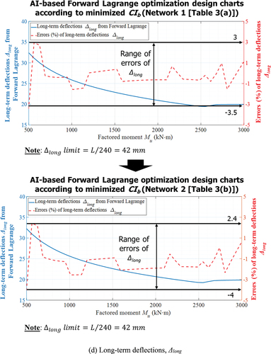
In this study, forward Lagrange networks were trained using PTM training method on nine input parameters (L, h, b, f_y,f^’_c, ρ_rt,ρ_rc,M_D,M_L) and eight outputs (ϕM_n,M_u,M_cr,Δ_imme,Δ_long,ε_{rt_0.003},ε_{rc_0.003},CI_b) with three layers based on (30, 40, and 50) neurons as indicated as Network 1* Table 3(a). Test mean-square errors (T.MSEs) of immediate and long-term deflections are improved when increasing a number of layers and neurons to four and five layers and (30, 40, 50, 60, and 70) neurons as shown in Network 2 Table 3(b). In* particular, T.MSE of Δ_imme (1.63E-4) and Δ_long (5.89E-5) with Network 1 is decreased slightly to 1.47E-4 and 5.64E-5, respectively, with Network 2 when a bigger number of layers and neurons is considered in Network 2. A number of layers (three layers) and neurons (40 neurons) are used for training ANN on Δ_imme and Δ_long in Network 1, whereas training ANNs on Δ_imme and Δ_long in Network 2 are conducted based on four layers with 40 neurons and five layers with 20 neurons, respectively, as shown in Table 3. The best training results for each parameter are presented in Table 3. The topology of forward Lagrange network was shown in Figure 4.

Figure 4. Topology of forward Lagrange network.

Figure 5

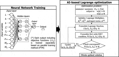
Figure 5. Verification of forward Lagrange network. (a) Factored moment (M_u) equality. (b) minimized cost index, CI_b. (c) Immediate deflections, Δ_imme. (d) Long-term deflections, Δ_long.

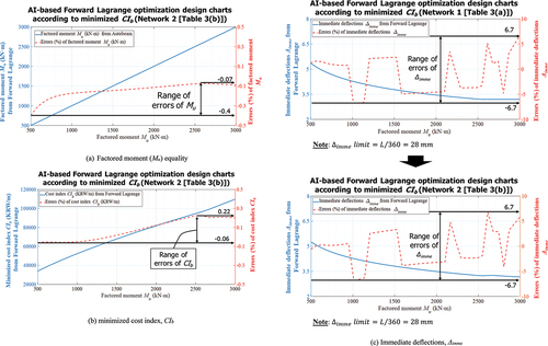
Figure 5. Continued.

4. Network verification

4.1. Verification of selected parameters including M_u (1.2M_D + 1.6M_L) equality based on forward Lagrange network

A forward Lagrange network optimizing cost (CI_b) of material and manufacture for design ductile beam sections shown in Figure 1 is verified in. A forward Lagrange network was formulated with eight forward output parameters (ϕM_n,M_u,M_cr,ε_{rt_0.003},ε_{rc_0.003},Δ_imme,Δ_long,CI_b) based on nine forward input parameters (L, h, b, f_y,f^’_c, ρ_rt,ρ_rc,M_D,M_L) as shown in Table 1. Verification of factored moment (M_u) minimized cost index (CI_b), immediate deflections (Δ_imme), and long-term deflections (Δ_imme) by structural engineering is shown in Figure 5.

Figure 5(a) demonstrates Lagrange network accuracies in terms of factored moment (including factored moment due to dead and live loads) set to between 500 and 3000 kN·m, which is established as an equality of the forward Lagrange network. Factored moment M_u obtained by network minimizing objective function (cost index, CI_b) was verified by structural calculation based on Autobeam software, which was used to generate large data. Range of errors of preassigned M_u compared to one calculated by structural engineering is from −0.4% to −0.07% as shown in Figure 5(a). Similarly, Figure 5(b) demonstrates minimized objective function (cost index, CI_b) which was established on output side of the forward Lagrange network. Cost index (CI_b) obtained by forward Lagrange network was verified by that found by structural calculation using design parameters obtained by network. The maximum error of cost index (CI_b) is 0.22% when M_u is equal to 2500 kN·m. Range of errors of preassigned M_u was between −0.4% and −0.07% as shown in Figure 5(a). Errors are negligible for the most of cost index (CI_b) as shown in Figure 5(b).

Although large errors (from −6.7% to 6.7% as shown in Figure 5(c)) compared with those based on structural engineering are found with immediate deflections for both Network 1 and 2, the absolute difference between network prediction and structural engineering calculation is insignificant. For example, Network 2 predicts an immediate deflection of 3.7 mm for M_u of 1000 kN·m when the error was largest as −6.7%, whereas one calculated based on structural engineering was 3.9 mm, resulting in only a 0.2 mm difference. On the other hand, range of errors of long-term deflections based on Network 1 is between −3.5% to 3%, which is improved slightly from −4% to 2.4% based on Network 2 as shown in Figure 5(d) when increasing a number of layers and neurons.

4.2. Verification of selected parameters based on large datasets

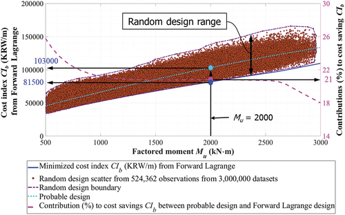
A number of 3,000,000 datasets were generated to verify optimization results based on Lagrange method. Verified big datasets were created by preassigning beam length, L, of 10 m, compressive concrete strength, f^’_c, of 30 MPa, yield strength of rebar, f_y, of 600 MPa, beam height, h, from 500 to 1200 mm, beam width, b, in the range from 0.3 to 0.5 times beam height. Then, factored moments, M_u, were sorted in the range of [500 ~ 3000] kN·m and design moment strength, ϕM_n, was selected from M_u to 1.2M_u. Moreover, design moment strength, ϕM_n, was constrained to be greater than 1.2 times cracking moment (1.2M_cr). Accordingly, a number of 524,362 datasets was selected from 3,000,000 datasets by considering constraints summarized in Table 5. It is worth noting that objective function (cost index, CI_b) was well minimized as verified by 524,362 datasets sorted from 3,000,000 datasets as shown in Figure 6. The network efficiency in saving a cost of beam material and manufacture is demonstrated with significant cost savings. As shown in Figure 6, cost distributions with random design ranges based on three million datasets were compared with those obtained by forward Lagrange networks, which predicted the lower bound of the cost index (CI_b). Optimization efficiencies with cost savings compared with probable designs which are established by considering safety factor of capacity from 1 to 1.2, that means range of design moment strength (ϕM_n) is bigger than factored moment (M_u) and less than 1.2 times M_u. Probable design as shown in Figure 6 was established by implementing the trend line function (“polyfit” and “polyval” commands) of MATLAB MathWorks (2020). The “polyfit” command returns coefficients for a function that is a best fit for the 524,362 datasets sorted from 3,000,000 datasets. The function of probable design, then, was obtained by “polyval” command based on the coefficients obtained by “polyfit” command.

Table 5. Constraints for verification datasets.

No.	Preassigned constraints
1	$L=10m$
2	${f_C}^{\prime }=30MPa$
3	$f_y=600MPa$
4	$h=\left[500\tilde{1}200\right]mm$
5	$=\left[0.3\tilde{0}.5\right]h$
No.	Sorted constraints
1	$M_u=\left[500\tilde{3}000\right]kN.m$
2	$\varphi M_n=\left[1\tilde{1}.2\right]M_u$
3	$\varphi M_n\ge 1.2M_{cr}$
4	${\epsilon }_{rt\mathrm{\_}0.003}\ge 0.004$
5	${\mathbf{\Delta }}_{imme}\le L/360=28mm$
6	${\mathbf{\Delta }}_{long}\le L/240=42mm$

Figure 6. Verification of optimized cost by 524,362 datasets from 3,000,000 datasets.

Figure 7a

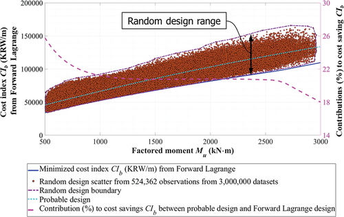
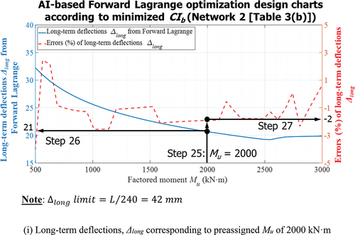
Figure 7. Application of AI, Lagrange-based design chart – Minimizing CI_b. (a) Cost index (CI_b) corresponding to preassigned M_u of 2000 kN·m. (b) Design moment ϕM_n corresponding to preassigned M_u of 2000 kN·m. (c) Cracking moment M_cr corresponding to preassigned M_u of 2000 kN·m. (d) Beam height (h) and beam width (b) corresponding to preassigned M_u of 2000 kN·m. (e) Tensile rebar (ρ_rt) and compressive rebar ratios (ρ_rc) corresponding to preassigned M_u of 2000 kN·m. (f) Tensile rebar strains, ε_{rt_0.003} corresponding to preassigned M_u of 2000 kN·m. (g) Compressive rebar strains, ε_{rc_0.003} corresponding to preassigned M_u of 2000 kN·m. (h) Immediate deflections, Δ_imme corresponding to preassigned M_u of 2000 kN·m. (i) Long-term deflections, Δ_long corresponding to preassigned M_u of 2000 kN·m.

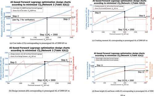
Figure 7. Continued.

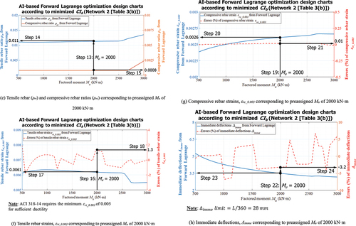
Figure 7. Continued.

5. Design charts based on forward Lagrange-based optimization

5.1. Cost (CI_b) optimization of material and manufacture for design ductile beam sections using design charts

AI-based design charts for beams shown in are shown with eight forward output parameters (ϕM_n,M_u,M_cr,ε_{rt_0.003},ε_{rc_0.003},Δ_imme,Δ_long,CI_b) based on nine forward input parameters (L, h, b, f_y,f^’_c, ρ_rt,ρ_rc,M_D,M_L) as shown in Table 1. Rebar ratios (ρ_rt and ρ_rc) determined as inequality constraints (refer to Table 2) minimized cost index (CI_b), eliminating engineers’ effort in predetermining rebar ratios (ρ_rt and ρ_rc). However, material properties and geometries should be predetermined by engineers. An RC beam was optimized with cost index (CI_b) based on forward Lagrange network. Saddle points were found based on Lagrange functions derived in Equation (4)(4) $\mathcal{L}\left(\mathbf{x},{\lambda }_c^T,{\lambda }_v^T\right)=f\left(\mathbf{x}\right)-{\lambda }_c^T\mathbf{c}\left(\mathbf{x}\right)-{\lambda }_v^T\mathbf{S}\mathbf{v}\left(\mathbf{x}\right)=C{I}_b-{\lambda }_c^T\mathbf{c}\left(\mathbf{x}\right)-{\lambda }_v^T\mathbf{S}\mathbf{v}\left(\mathbf{x}\right)$(4) . KKT conditions were applied to consider inequality constraints as shown in Equation (6)(6) $\mathrm{\nabla }\mathcal{L}\left(\mathbf{x},{\lambda }_c,{\lambda }_v\right)=\left[\begin{array}{c}\begin{array}{c}\mathrm{\nabla }f\left(\mathbf{x}\right)-J_{\mathbf{c}}{\left(\mathbf{x}\right)}^T{\lambda }_c-J_{\mathbf{v}}{\left(\mathbf{x}\right)}^T\mathbf{S}{\lambda }_v\\ -\mathbf{c}\left(\mathbf{x}\right)\end{array}\\ -\mathbf{S}\mathbf{v}\left(\mathbf{x}\right)\end{array}\right]$(6) .

5.2. Use of design charts to design ductile beam sections

Design example is shown with preassigned beam dimensions (L = 10,000 mm) and beam material properties (f_y = 600 MPa and f^’_c = 30 MPa). Load demands are also prescribed as M_D = 1000 kN·m, M_L = 500 kN·m, M_u = 1.2M_D + 1.6M_L = 2000 kN·m. Figure 7(a) shows minimized CI_b can be selected directly from design charts based on Lagrange optimization. The rest of design parameters corresponding to a specified factored moment (M_u) of 2000 kN·m can be found using design charts shown in Figure 7, helping engineers to be aware of design parameters with insignificant errors. Final beam design obtained in Figure 8 shows beam section (width, b and height, h), rebar ratios (ρ_rt and ρ_rc), and locations of both tension and compression reinforcements, from which the neutral axis can also be calculated.

Figure 8. Final beam design corresponding to preassigned M_u of 2000 kN⋅m.

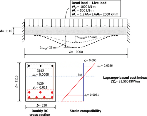
For steps 1 to 3 (Figure 7(a)), forward Lagrange-based optimization charts to determine minimized CI_b are entered with factored moment M_u of 2000 kN·m with which beam section (width, b and height, h), and rebar ratios (ρ_rt and ρ_rc). The minimized CI_b of 81,500 KRW/m according to preassigned M_u of 2000 kN·m is selected with a corresponding error of CI_b of 0.12%. Step 4 (Figure 7(b)) supports engineers to move to axis for determining design moment (ϕM_n) corresponding to preassigned M_u of 2000 kN·m. Design moment (ϕM_n) and associated error are obtained of 2000 kN·m and 1.1%, respectively, in Steps 5 and 6 for preassigned M_u of 2000 kN·m. Cracking moment (M_cr) and the corresponding error are obtained of 300 kN·m and 0.12% similarly to Steps 7 to 9 (Figure 7(c)). Step 10 (Figure 7(d)) assists engineers to move to axes for determining beam height, h, and beam width, b, for preassigned factored moment M_u. A beam height, h, of 1110 mm and a beam width, b, of 330 mm are selected in Steps 11 and 12 (Figure 7(d)), respectively. For Steps 13 to 15 (Figure 7(e)), a compressive rebar ratio (ρ_rc) of 0.0008 and a tensile rebar ratio (ρ_rt) of 0.011 are determined, similarly. A tensile rebar strain (ε_{rt_0.003}) of 0.0061 and a compressive rebar strain (ε_{rc_0.003}) of 0.0026 for a specified factored moment (M_u) of 2000 kN·m are identified with the corresponding errors as shown in Steps 16 to 21* Figure 7(f,g) where acceptable accuracies are demonstrated as compared with calculations based on engineering mechanics. ACI 318–14 Standard (2014) recommends that tensile rebar ratios decrease to increase rebar strains when tensile strains of rebars (ε_{rt_0.003}) are less than 0.004. The design charts shown in Figure 7(f) help engineers to be aware of design parameters, as required by codes. Design requirements imposed by codes (including ACI 318–14, Section 9.3.3.1 Standard (2014)) are reflected by inequality constraints. The design parameters meeting this requirement can be achieved by selecting design parameters corresponding to tensile strains of rebars (ε_{rt_0.003}) greater than 0.004 as shown in ((Figure 7(f)) with equality constraints including L =10,000 mm, f_y =600 MPa, and f’_c =30 MPa. Figure 7(f) also demonstrates how design charts are used to design tension-controlled ductile beam sections with strains greater than 0.005. Steps 22 to 27 Figure 7(h,i) let engineers find an immediate deflection Δ_imme of 3.5 mm and a long-term deflection Δ_long of 21 mm with the corresponding errors when factored moment (M_u) reaches 2000 kN·m. Final beam design corresponding to preassigned factored moment (M_u) with optimized CI_b is illustrated in Figure 8. As shown in Figure 9, cost index of a beam CI_b (81,500 KRW/m) based on Lagrange network reduced to 21% from probable design values (103,000 KRW/m). Any reverse parameter to be pre-assigned is trained in input. Engineers can pre-assign parameters as constraining conditions of interests. Notably, this type of reverse technique can be implemented to control ductility of frames, helping engineers to predetermine performance level of frames by pre-determining ductility (in terms of strains) for seismic design. However, design charts similar to Figures 5 and Figure 7 can be constructed based on any reverse parameters which are pre-assigned and trained on input side. Design charts similar to Figures 5 and Figure 7 can serve as a rapid and accurate reference, investigating a structural behavior of beam sections, and ensuring to meet code requirements. Well-balanced designs are now possible based on the proposed AI-based design technologies to optimize objective function of any type, whereas it has been challenging to perform reverse designs based on conventional beam design.

Figure 9. Verification of cost effectiveness of M_u = 2000 kN·m.

5.3. Verification of cost-effectiveness

Figure 9 compares cost index (CI_b) of beams with 524,362 datasets sorted from 3,000,000 large datasets based on constraints as shown in Table 5, eliciting that Lagrange functions were well optimized for designing RC beams, where cost reductions over 18–26% are demonstrated compared with probable beam designs. Contributions (%) to cost index (CI_b) of a beam decreases as design beam capacities increase. Design accuracies are demonstrated as shown in Table 6 where design errors were negligible for practical applications. A Lagrange-based cost index (CI_b = 81,500 KRW/m) of a beam with factored moment (M_u) of 2000 kN·m was compared to cost index (CI_b = 103,000 KRW/m) based on a probable design as shown in Figure 9.

Table 6. Design table corresponding to preassigned M_u of 2000 kN⋅m.

AI-based Forward Lagrange optimization according to minimized CIb 9 Inputs (L, h, b, fy,f^’c, ρrt,ρrc,MD,ML) – 8 Outputs (ϕMn,Mu,Mcr,εrt_0.003,εrc_0.003,Δimme,Δlong,CIb)
No.	Parameter	Forward Lagrange (PTM)	Error (%)
1	L (mm)	10,000	-
2	h (mm)	1110	-
3	b (mm)	330	-
4	fy (MPa)	600	-
5	f^’c (MPa)	30	-
6	ρrt	0.0110	-
7	ρrc	0.00080	-
8	MD (kN⋅m)	1000	-
9	ML (kN⋅m)	500	-
10	ϕMn (kN⋅m)	2000.0	1.10%
11	Mu (kN⋅m)	2000.0	−0.11%
12	Mcr (kN⋅m)	300.0	0.12%
13	εrt_0.003	0.0061	1.30%
14	εrc_0.003	0.0026	0.01%
15	Δimme (mm)	3.5	−3.20%
16	Δlong (mm)	21	−2.00%
17	CIb (KRW/m)	81,500	0.12%

–

• Forward inputs parameters: No. 1 ~ 9

–

• Forward outputs parameters: No. 10 ~ 17

6. Results and discussions

6.1. AI-based formulation of objective functions based on large datasets

(1) AI-based cost objective function as a function of nine forward input parameters was formulated to replace complex mathematical and analytical objective functions. AI-based networks mapped network input to output parameters, deriving objective functions which are led to Lagrange functions with equality and inequality constraints.

(2) Obtaining analytical objective functions for design target which can represent accurate structural behavior as a function of multiple design parameters (nine forward input parameters (L, h, b, f_y,f^’_c, ρ_rt,ρ_rc,M_D,M_L) for doubly reinforced concrete (RC) beams) is difficult, limiting an application of Lagrange optimization.

(3) This study developed ANN-based forward Lagrange networks optimizing ductile doubly reinforced concrete (RC) beams. An objective function representing cost (CI_b) of materials and manufacture established as one the most favorable design targets was minimized based on six equality and 11 inequality constraints which were implanted as artificial neural genes according to engineer’s needs.

6.2. Design charts obtained based on Lagrange networks optimizing cost (material and manufacture) of ductile doubly reinforced concrete (RC) beam

(1) AI-based design charts for beams shown in Figure 7 were developed with eight forward output parameters (ϕM_n,M_u,M_cr,ε_{rt_0.003},ε_{rc_0.003},Δ_imme,Δ_long,CI_b) based on nine forward input parameters (L, h, b, f_y,f^’_c, ρ_rt,ρ_rc,M_D,M_L) shown in Table 1.

(2) Sequence of selecting parameters including material properties and geometries were arbitrarily determined by users. The design targets (objective functions) are governed by equality and inequality conditions based on design conditions.

(3) Users can construct design charts based on any type of design charts and object functions where design parameters were constrained by equality and inequality conditions.

6.3. Verifying optimized objective functions

(1) Proposed neural networks based on Lagrange optimization offered a design for ductile doubly reinforced beams that made cost of beam material and manufacture least. As shown in Figure 7, shallow neural networks were formulated to provide the most favorable designs for safety and economy, while being verified by large datasets.

(2) Predictions of network outputs were verified as closely to those calculated by engineers as shown in Table 6. Close correlations between network outputs and design results based on mechanics were demonstrated for given beam properties and geometries.

(3) The future study should delve deeper into for minimizing CO₂ emissions of RC beams, contributing to solving the specific needs that may help industries at the time of climate changes. Complex optimization of diverse design problems such as columns, slabs, foundations, and pre-stressed beams is to be performed, which are challenging to solve by mathematical optimization techniques.

6.4. Structural designs beyond human efficiency

6.4.1. Design efficiencies

Networks contributed to fast and accurate designs, offering structural designs which were more effective than those designed by human engineers. Lagrange functions were placed with constraining conditions in ANN to automatically determine the most efficient beam designs leading to the cost of beams lower than one achieved by humans.

6.4.2. Generation of large datasets with good quality

All design information was delivered to AI networks via large datasets. So is a quality of large datasets the most important, encouraging engineers to prepare codes to generate datasets of good quality. AI remembers entire data trend including correlations and cross-parametric behaviors through recognizing datasets and recalls them for designs beyond human efficiency.

7. Conclusions

AI-based design is capable of providing many creative ways, such as saving endeavor and time for engineers while acquiring design solutions beyond what they intend. AI-based design can replace conventional design methods, eventually making structural designs free from human effort, judgment, and errors. This study demonstrated that analytical objective functions were replaced by those obtained based on large data to achieve optimized designs based on Lagrange functions. ANNs-based forward Lagrange networks were formulated to optimize ductile doubly reinforced concrete (RC) beams. An AI-based objective function was established to minimize Cost (CI_b) of materials and manufacture, based on constraints in accordance with both design codes and engineer’s needs. Large datasets of 100,000 were utilized to derive an AI-based objective function for cost (CI_b, minimizing cost of RC beams) as a function of forward input parameters, enabling to replace complex analytical objective functions. Cost reductions from Lagrange optimization from 18% to 26% are observed compared with probable beam designs obtained from 524,362 observations from 3,000,000 datasets as shown in Figure 6. Conventional computations based on structural mechanics were used to ascertain the network’s results. This study proposed an AI-based Lagrange optimization design charts according to minimized CI_b which can deliver fast but accurate initial designs to engineering practice.

Disclosure statement

No potential conflict of interest was reported by the author(s).

Supplemental Material

Supplemental data for this article can be accessed here

Correction Statement

This article has been republished with minor changes. These changes do not impact the academic content of the article.

Additional information

Funding

This work was supported by the National Research Foundation of Korea (NRF) grant funded by the Korean government [MSIT 2019R1A2C2004965].

References

- Adeli, H. 2001. “Neural Networks in Civil Engineering: 1989–2000.” Computer‐Aided Civil and Infrastructure Engineering 16 (2): 126–142. doi:10.1111/0885-9507.00219.
- Aghaee, K., M. A. Yazdi, and K. D. Tsavdaridis. 2014. “Mechanical Properties of Structural Lightweight Concrete Reinforced with Waste Steel Wires.” Magazine of Concrete Research 66 (1): 1–9.
- Ahmadi, N., R. Moghadas, and A. Lavaei. 2008. “Dynamic Analysis of Structures Using Neural Networks.” American Journal of Applied Sciences 5 (9): 1251–1256. doi:10.3844/ajassp.2008.1251.1256.
- Awal, A. A., I. A. Shehu, and M. Ismail. 2015. “Effect of Cooling Regime on the Residual Performance of High-volume Palm Oil Fuel Ash Concrete Exposed to High Temperatures.” Construction and Building Materials 98: 875–883. doi:10.1016/j.conbuildmat.2015.09.001.
- Fahmy, A. S., E.-M. Met, and Y. A. Gobran. 2016. “Using Artificial Neural Networks in the Design of Orthotropic Bridge Decks.” Alexandria Engineering Journal 55 (4): 3195–3203. doi:10.1016/j.aej.2016.06.034.
- Fanaie, N., S. Aghajani, and E. A. Dizaj. 2016. “Theoretical Assessment of the Behavior of Cable Bracing System with Central Steel Cylinder.” Advances in Structural Engineering 19 (3): 463–472. doi:10.1177/1369433216630052.
- Fanaie, N., S. Aghajani, and S. Shamloo. 2012. “Theoretical Assessment of Wire Rope Bracing System with Soft Central Cylinder.” Proceedings of the 15th World Conference on Earthquake Engineering.
- Flood, I., and N. Kartam. 1994a. “Neural Networks in Civil Engineering. I: Principles and Understanding.” Journal of Computing in Civil Engineering 8 (2): 131–148. doi:10.1061/(ASCE)0887-3801(1994)8:2(131).
- Flood, I., and N. Kartam. 1994b. “Neural Networks in Civil Engineering. II: Systems and Application.” Journal of Computing in Civil Engineering 8 (2): 149–162. doi:10.1061/(ASCE)0887-3801(1994)8:2(149).
- Gomes, G. F., F. A. de Almeida, D. M. Junqueira, S. S. da Cunha Jr, and A. C. Ancelotti Jr. 2019. “Optimized Damage Identification in CFRP Plates by Reduced Mode Shapes and GA-ANN Methods.” Engineering Structures 181: 111–123. doi:10.1016/j.engstruct.2018.11.081.
- Gupta, T., and R. K. Sharma. 2011. “Structural Analysis and Design of Buildings Using Neural Network: A Review.” International Journal of Engineering and Management Sciences 2 (4): 216–220.
- Heydari, A., and M. Shariati. 2018. “Buckling Analysis of Tapered BDFGM Nano-beam under Variable Axial Compression Resting on Elastic Medium.” Structural Engineering & Mechanics 66 (6): 737–748. doi:10.12989/sem.2018.66.6.737.
- Hong, W. K. 2019. Hybrid Composite Precast Systems: Numerical Investigation to Construction, 427–478. Woodhead Publishing, Elsevier.
- Kaveh, A., and F. Shokohi. 2015. “Optimum Design of Laterally Supported Castellated Beams Using CBO Algorithm.” Steel & Composite Structures 18 (2): 305–324. doi:10.12989/scs.2015.18.2.305.
- Korouzhdeh, T., H. Eskandari-Naddaf, and M. Gharouni-Nik. 2017. “An Improved Ant Colony Model for Cost Optimization of Composite Beams.” Applied Artificial Intelligence 31 (1): 44–63. doi:10.1080/08839514.2017.1296681.
- Krenker, A., J. Bešter, and A. Kos. 2011. “Introduction to the Artificial Neural Networks.” Artificial Neural Networks: Methodological Advances and Biomedical Applications. InTech 1–18. doi:10.5772/15751.
- Kuhn, H. W., and A. W. Tucker. 1951. Nonlinear Programming. Berkeley Symposium on Mathematical Statistics and Probability.
- Lee, S., J. Ha, M. Zokhirova, H. Moon, and J. Lee. 2018. “Background Information of Deep Learning for Structural Engineering.” Archives of Computational Methods in Engineering 25 (1): 121–129. doi:10.1007/s11831-017-9237-0.
- Madadi, A., H. Eskandari-Naddaf, R. Shadnia, and L. Zhang. 2018. “Characterization of Ferrocement Slab Panels Containing Lightweight Expanded Clay Aggregate Using Digital Image Correlation Technique.” Construction and Building Materials 180: 464–476. doi:10.1016/j.conbuildmat.2018.06.024.
- MathWorks. 2020. MATLAB R2020b, Version 9.9.0. Natick, Massachusetts: MathWorks.
- MathWorks. 2020a. “Deep Learning Toolbox: User’s Guide (R2020a).” Accessed 26 July 2020. https://www.mathworks.com/help/pdf_doc/deeplearning/nnet_ug.pdf
- MathWorks. 2020b. “Parallel Computing Toolbox: Documentation (R2022a).” Accessed 26 July 2020. https://uk.mathworks.com/help/parallel-computing/
- MathWorks. 2020c. “Statistics and Machine Learning Toolbox: Documentation (R2020a).” Accessed 26 July 2020. https://uk.mathworks.com/help/stats/
- MathWorks. 2020d. “Global Optimization: User’s Guide (R2020a).” Accessed 26 July 2020. https://www.mathworks.com/help/pdf_doc/gads/gads.pdf
- MathWorks. 2020e. “Optimization Toolbox: Documentation (R2020a).” Accessed 26 July 2020. https://uk.mathworks.com/help/optim/
- Nasrollahi, S., S. Maleki, M. Shariati, A. Marto, and M. Khorami. 2018. “Investigation of Pipe Shear Connectors Using Push Out Test.” Steel & Composite Structures 27 (5): 537–543. doi:10.12989/scs.2018.27.5.537.
- Nguyen, D. H., W. K. Hong, and I. Part. 2019. “The Analytical Model Predicting Post-Yield Behavior of Concrete-Encased Steel Beams considering Various Confinement Effects by Transverse Reinforcements and Steels.” Materials 12 (14): 2302. doi:10.3390/ma12142302.
- Paknahad, M., M. Bazzaz, and M. Khorami. 2018. “Shear Capacity Equation for Channel Shear Connectors in Steel-concrete Composite Beams.” Steel & Composite Structures 28 (4): 483–494. doi:10.12989/scs.2018.28.4.483.
- Rizzo, F., and L. Caracoglia. 2020. “Artificial Neural Network Model to Predict the Flutter Velocity of Suspension Bridges.” Computers & Structures 233: 106236. doi:10.1016/j.compstruc.2020.106236.
- Safa, M., M. Shariati, Z. Ibrahim, A. Toghroli, S. B. Baharom, N. M. Nor, and D. Petkovic. 2016. “Potential of Adaptive Neuro Fuzzy Inference System for Evaluating the Factors Affecting Steel-concrete Composite Beam’s Shear Strength.” Steel & Composite Structures 21 (3): 679–688. doi:10.12989/scs.2016.21.3.679.
- Shah, S. N. R., N. R. Sulong, R. Khan, M. Z. Jumaat, and M. Shariati. 2016. “Behavior of Industrial Steel Rack Connections.” Mechanical Systems and Signal Processing 70–71: 25–740. doi:10.12989/scs.2016.21.3.679.
- Shariat, M., M. Shariati, A. Madadi, and K. Wakil. 2018. “Computational Lagrangian Multiplier Method by Using for Optimization and Sensitivity Analysis of Rectangular Reinforced Concrete Beams.” Steel & Composite Structures 29 (2): 243–256. doi:10.12989/scs.2018.29.2.243.
- Shariati, M., S. N. H. Ramli, S. Maleki, and M. M. Arabnejad Kh. 2010. “Experimental and Analytical Study on Channel Shear Connectors in Light Weight Aggregate Concrete.” Proceedings of the 4th International Conference on Steel & Composite Structures, 21–23. https://doi.org/10.3850/978-981-08-6218-3_CC-Fr031.
- Standard, A. A. 2014. Building Code Requirements for Structural Concrete (ACI 318–14). In American Concrete Institute.
- Toghroli, A., M. Mohammadhassani, M. Suhatril, M. Shariati, and Z. Ibrahim. 2014. “Prediction of Shear Capacity of Channel Shear Connectors Using the ANFIS Model.” Steel & Composite Structures 17 (5): 623–639. doi:10.12989/scs.2014.17.5.623.
- Upton, G., and I. Cook. 2014. A Dictionary of Statistics 3e. Oxford University Press.
- Villarrubia, G., J. F. De Paz, P. Chamoso, and F. De la Prieta 2018. “Artifcial Neural Networks Used in Optimization Problems.” Neurocomputing 272: 10–16. doi:10.1016/j.neucom.2017.04.075
- Wu, R. T., and M. R. Jahanshahi. 2019. “Deep Convolutional Neural Network for Structural Dynamic Response Estimation and System Identification.” Journal of Engineering Mechanics 145 (1): 04018125. doi:10.1061/(ASCE)EM.1943-7889.0001556.