Couple simulations with CFD and ladybug + honeybee tools for green façade optimizing the thermal comfort in a transitional space in hot-humid climate

ABSTRACT

Vertical gardens have become important strategies for urban heat island migration in recent years. However, the simulation tools for green façade (GF) with climbing plants coupling the shading and wind-induced effects are still lacked. This study focused on GF effects on human thermal comfort (HTC) optimization in a transitional space. The main purpose was to develop a couple method on HTC simulations. Field measurements in a hot-humid climate area were conducted to obtain the parameters of GF foliage layers. A couple simulation method with Ansys Fluent, Ladybug, and Honeybee tools was developed. Seven GFs layouts on a standard balcony model were simulated. In field measurements, the Ave. global irradiation was reduced by 73.29%, leaf area index was measured at 1.56–3.61, and foliage cover ratio was measured at 49.74–92.88%. In the simulations, the results of the Ave. wind velocity were reduced by 0.20–0.77 m s⁻¹, the Ave. air temperature was reduced by 0.2°C, the Ave. mean radiant temperature was reduced by 0.5–7°C, and the Ave. physiological equivalent temperature was reduced by 0.3–3.2°C. The couple method could support the architectural and landscape design integrating with the GFs in future.

GRAPHICAL ABSTRACT

KEYWORDS:

• Green facade
• thermal comfort
• CFD
• couple simulation
• transitional space

1. Introduction

Global climate change and the urban heat island (UHI) effect have become much more serious in recent years. Urban sprawl has also led to a rapid decrease in green urban land. In response to these challenges, urban greenery infrastructure (UGI) strategies, which will improve urban climate, urban health, and urban resilience, have been introduced to policymakers and urban planners. The UGI, which includes a multiscale of green lands and vertical greenery spaces such as urban parks, pocket gardens, vertical gardens, green roofs, and green walls, has been rapidly promoted for UHI migration and healthy city policies (Zölch et al. 2016).

In high-density urban areas, vertical greening (VG) strategies have become important methods of addressing the lack of green land. Different strategies of VGs are promoted depending on the urban environment (Pérez et al. 2014). Green roofs (GR) and green walls (GW) are the two main strategies for VG. GRs have been demonstrated to improve energy saving, rainwater preservation, air quality improvement, and UHI mitigation (Liu et al. 2021; Coma et al. 2017). Although GWs have a long history, they have developed fast in recent years due to UHI mitigation, prefabrication technologies, and urban greening support policies (Aflaki et al., 2017). GWs mainly consist of two systems: the living wall system (LWS) and the green façade (GF). Cross-climate zones and season studies on GWs have demonstrated the potential for energy saving, improving the thermal environment (Coma et al. 2017), noise insulation, dust reduction, and biological diversity promotion (Köhler 2008; Sheweka and Mohamed 2012).

Regarding the thermal environment, human thermal comfort (HTC) is an important issue in high-density urban areas. Recent studies of GWs have demonstrated the positive effect of GWs on HTC via the shading effects of solar radiation, the reduction of surface heat reflection, and the evaporation effects of plant and substrate (Table 1). However, despite the increasing application and various design patterns available for GWs, we still lack meaningful design-supported tools and evaluation methods for GWs, particularly for the determination of building performance in terms of architectural and landscape design.

Table 1. GFs’ effects on thermal environment in different climate zones.

Photos of measurements	Location	S*	KCC**	Results	Photos of measurements	Location	S	KCC	Results
Global irradiation (Ga)					Wall external surface temperature (Ts)
	Hong Kong, China	Sum	Cfa	–Max. 300 W m^−2 Transmittance: 37.1% (Jim 2015a)		Singapore	Sum	Af	–Max. 2.45 °C (Wong et al. 2010)
	Ljubljana, Slovenia	Sum	Cfb	Transmittance: 23.3% (Šuklje, Medved, and Arkar 2016)		Chicago, America	Sum	Dfa	–0.7–13.1 °C (Susorova, Azimi, and Stephens 2014)
	Saitama, Japan	Sum	Cfa	–600 W m^−2 (South) (Koyama et al. 2015)		Thessaloniki, Greek	Sum	Csa	–16.85 °C (West) –10.53 °C (East) –6.46 °C (South) (Kokogiannakis et al. 2019)
	Malaysia	Spr	Af	–Max. 486.9 W m^−2 Transmittance: 29.1–42.9% (Sulaiman, Jamil, and Zain 2013)		Puigverd de Lleida, Spain	Sum	Csa	–Ave. 13.9 °C (West) –Ave. 13.8 °C (East) –Ave. 10.7 °C (South) (Coma et al. 2017)
	Munich, Germany	Sum	Dfb	–Ave. 84.9 W m^−2 (Cloudy) –Ave. 391.4 W m^−2 (Clear) Transmittance: 11.6–29.8% (Lin, Musso, and Xiao 2018)		Guangzhou, China	Sum	Cfa	–Ave. 4.7 °C (East) (Lin, Xiao, and Musso 012006)
	Guangzhou, China	Sum	Cfa	Transmittance: Approx. 50% (Zhang et al. 2019)		Bari, Italy	Al	Csa	–Max.9.0 °C (Vox, Blanco, and Schettini 2018)
Air temperature (Ta) in the cavity					Wind velocity (Va) in the cavity
	Saitama, Japan	Sum	Cfa	–Max. 2 °C (Koyama et al. 2015)		Delft, Netherlands	Sum	Cfb	–Ave. 0.2 m s^−1 –Max. 0.69 m s^−1 (Perini et al. 2011)
	Delft, Netherlands	Sum	Cfb	–Ave. 1.26 °C –Max. 1.39 °C (Perini et al. 2011)		Delft, Netherlands	Sum	Cfb	–Ave. 0.12 m s^−1 –Max. 0.40 m s^−1 (Perini et al. 2011)
	Guangzhou, China	Sum	Cfa	–Ave. 0.5 °C (East) –Ave. 0.7 °C (South) –Max. 3.2 °C (East) –Max. 3.8 °C (South) (Lin, Xiao, and Musso 012006)		Guangzhou, China	Sum	Cfa	–Ave. 0.8 m s^−1 –Max. 2.7 m s^−1 (Lin et al. 2019)
	Guangzhou, China	Sum	Cfa	–Ave. 0.53 °C (South) –Max. 1.14 °C (South) (Lin et al. 2019)		Munich, Germany	Sum	Dfb	–Ave. 0.7 m s^−1 –Max. 2.7 m s^−1 (Lin, Musso, and Xiao 2018)
	Munich, Germany	Sum	Dfb	–Ave. 1.9 °C (West) –Max. 3.8 °C (West) (Lin, Musso, and Xiao 2018)

*S, Season: Sum, summer; Spr, spring; Al, all year.

**KCC: Köppen climate classification (Köppen 2011): Dfa,Dfb, Humid continental climate; Af, Tropical rainforest climate; Cfb, Temperate oceanic climate; Cfa, Humid subtropical climate; Csa, Hot-summer Mediterranean climate; Csb, Warm-summer Mediterranean climate.

This study is mainly focused on the GFs’ effects on HTC. GFs mainly allow the climbing plants to grow vertically via specific lightweight structures and help them form shading screens with their foliage layers (2010Façade Planting [n] 2010]. With the porous character of the foliage layers, the GFs provide shade and wind-induced effects on HTC optimization (Jim 2015b). GFs are widely grown on the external surfaces of building walls, sky gardens, and balconies. GFs can be implemented in various scenarios because of their low cost of planting, maintenance, and simple structure (Perini and Rosasco 2013). Furthermore, different species of climbing plants support high adaptability in different climates (Isnard and Silk 2009; Paul and Yavitt 2011).

In south China’s hot and humid climate, the hot months have been increasing in recent years, highlighting the critical need for HTC optimization. GFs can aid in this endeavor, especially for residential buildings, where the local habitants can add plants and simple shading devices on building facades or balconies, which is particularly relevant in the fast-developing, dense urban environment. The number of residential buildings in dense urban environments increased extremely fast due to China’s urbanization trend in the last 30 years. In a residential building, the balcony space is the specific space between outdoor and indoor environments and supports various activities, such as clothes drying, growing gardens, resting, and dining. As climbing plants are widely applied in balcony gardens, this study takes balcony GFs as a climate adaptation strategy for hot and humid climates; to achieve this, we set up a research target to evaluate the effects on HTC. Determining the thermal comfort and temperature control of specific GF design patterns Figure 1 would support the future architectural and landscape design of GFs in a wider background.

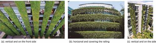
Figure 1. Cases of GFs layouts on corridors and balconies.

In this research area, a balcony could be defined as one of the typologies of transitional space as well, which is a space between the outdoors and indoors with different enclosed elements, such as roofs and walls, reducing the effects of solar radiation on human beings (Chun and Tamura 2005; Chun, Kwok, and Tamura 2004). In hot and humid climate areas, the transitional spaces, such as corridors, arcades, and atriums, support various activities of commerce, leisure, community, and children playing (Zhang, Zhang, and Ding 2017); thus, this combination study on balconies with different GFs patterns would deepen the understanding of the optimization strategies for the transitional spaces and extend the possibility for people staying in these spaces despite the high temperature and strong solar radiation in summer.

This research is based on a previous study of GF effects on HTC in the hot and humid climate in southern China (China Meteorological Administration (in Chinese) 2021). The previous study of GFs had conducted field measurements on thermal comfort indices. A computational fluid dynamics (CFD) method was also developed, validated, and then simulated on different patterns of foliage distribution on a standard building with a transitional space (Lin et al. 2019), testing the GFs’ regulations on air temperature (T_a) and wind velocity (V_a); however, the evaluation of HTC in a transitional space needs to consider the T_a and V_a and take into account the global irradiation (G_a), human activity, clothing, and the relative humidity (RH). A better evaluation method for HTC in a transitional space in a hot and humid climate is to introduce the index of physiological equivalent temperature (PET) (Höppe 1999), which is the temperature of a reference environment based on a heat balance model that combines various climatic and physiological variables including T_a, RH, solar and environmental thermal radiation, V_a, clothing, and metabolic rate to provide a synergetic indicator of HTC (Mayer and Höppe 1987). This index is widely used to understand the thermal comfort environment of outdoor spaces and has been tested and validated in local field measurements and questionnaire surveys in the hot and humid climate in southern China (Zhang, Zhang, and Ding 2017; Zhang, Zhang, and Jin 2018). Furthermore, considering a balcony space with GF would be affected by solar radiation, the index of PET is much more suitable than some HTC indices such as PMV-PPD utilizing in an indoor environment. In this study, we aimed to develop a coupled method to calculate the PET based on CFD simulations and evaluate the HTC level on balconies in summer.

2. Methodology

In the previous study (Lin et al. 2019), the GFs’ effects on HTC had been discussed via field measurements and CFD simulations. The field measurements were taken in a corridor of an apartment in summer in Guangzhou, China. In the CFD simulations, the indices of T_a and V_a were validated and simulated with different façade layouts, preliminarily discussing the shading and wind-induced effect of the GFs in the transitional space. As introduced above, a much more comprehensive evaluation of HTC should include various indices; therefore, the method of the previous study requires improvement.

As the previous study revealed, T_g, T_r, and PET indices showed high correlations in the field measurements, which implied that the solar radiation provided a strong effect on HTC and the foliage layer of the GFs provided an effective shading effect improving the HTC (Lin et al. 2019); thus, we conducted a study on the effects of GFs on solar radiation. First, the shading effect was estimated with the coverage indices of the foliage layer of the GFs, which are the key parameters for the solar radiation simulation. Second, the coverage indices were set in the previous standard CFD model to test the shading and evaporation effects separately. At the same time, the models of the various GF layout typologies on a standard balcony model were constructed based on cases studies. Fourth, based on the standard parameters of the GFs’ foliage layer and the standard CFD models, a couple simulation method was introduced, tested, and provided a deeper study into HTC.

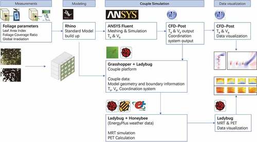
The methods implemented in this study consist of 4 main steps: 1. The field measurements of GFs’ foliage parameters; 2. standard model definitions for GFs simulation; 3. the setting of CFD simulations; 4. the couple simulation with solar radiation and calculation for PET.

This study was performed in Guangzhou, China. Guangzhou is located in southern China (23°08ʹN, 113°16ʹE); in summer, the average high temperature is 32.3 °C, and the average relative humidity is 83% (China Meteorological Administration (in Chinese) 2021). Guangzhou has a humid subtropical climate according to the Köppen climate classification (KCC) (Köppen 2011). The experiment was conducted in June. 2019 and the simulations was set on 22^nd June, which is a typical summer day in hot-humid climate.

2.1. Field measurements of GFs’ foliage parameters

The shading effect of the GFs was estimated in two aspects. First, the solar radiation was measured behind and outside the foliage layer to compare the reduction ratio. Second, the coverage ratio of the foliage indices were measured to obtain the foliage preference.

2.1.1. Measurements of solar radiation

Field measurements of solar radiation were taken over ten days in June and an index of G_a was recorded by the HD 31 with a LP471 SILICON-PYRA probe (Figure 2(a) and Table 2). The measurement period had covered the different weather characters of cloudy and sunny days, then, we stopped the measurement before a rainy day to protect the experiment probes. As the foliage layer of a GF is distributed vertically, the measurements of the GFs were conducted horizontally behind the GFs with a distance of 0.3 m at the height of 0.6 m, 0.9 m, 1.2 m, 1.5 m, 1.8 m, and 2.1 m, recording the foliage character in the height range of a human being. The capacity of the G_a adjustment of the foliage layer was analyzed and integrated into the simulation model.

Figure 2. Instruments for the GFs’ foliage layer measurements.

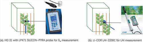
Table 2. Instruments for the GFs’ foliage index measurements.

Instrument	Index	Range	Accuracy
HD 31 with LP471 SILICON-PYRA probe	Global irradiation (Ga)	Spectral range:400–1100 nm	1.0–19.99 W m^−2, 0.001 W m^−2; 20.0–199.00 W m^−2, 0.01 W m^−2; 200.0–1999.0 W m^−2, 0.1 W m^−2
LI-COR LAI-2200C	Leaf area index (LAI)	Wavelength Range: 320–490 nm	> 99% from 490–650 nm; > 99.9% above 650 nm

2.1.2. Measurements of the coverage ratio of the GFs’ foliage layer

In the literature, the measurements of the foliage distribution could be described as foliage coverage ratio (FCR) or leaf area index (LAI) (Jonckheere et al. 2004; Hunt et al. 2013; Azhar Mat Sulaiman et al. 012025; Casadesús and Villegas 2014; Pérez et al. 2017). The former method is based on applications in agriculture and remote-sensing areas, which compares the color pixels of the plants to the surrounding environment. The color range of the foliage was built up under the empirical measurements (Hunt et al. 2013; Azhar Mat Sulaiman et al. 012025; Casadesús and Villegas 2014); however, the foliage color may be different in different species and seasons, which may also increase the probability of errors in the measurements. Both a photo background with high color contrast and a color range recording in situ for the specific plants’ foliage are needed in field measurements to decrease the likelihood of error. The latter method mainly compares the solar radiation values of the space in an open space to values collected behind the foliage layer to calculate the shading level of a crown of a plant (Jonckheere et al. 2004; Pérez et al. 2017). This method is also widely applied in agriculture and forest management, as well as research; however, most LAI measurements were measured on a horizontal surface, as the crowns of the trees are mainly distributed vertically. The climbing plants of the GFs normally grow on a vertical surface, and as such, measurements should be taken on a vertical surface, which is often not performed in field measurements.

To compare both methods, we investigated both indices simultaneously with the same plants. To reduce the inference of the surrounding environment, the GFs were chosen on a building with a bare wall as a contrasting background. The measurements were taken at both positions of the shading area of the plants and the open space. The photos of the FCR of the GFs were processed with a photo pixel analysis program (Adobe Photoshop). The LAI values of the GFs were measured with the equipment of LI-COR LAI-2200C (Figure 2(b) and Table 2). Finally, the data taken from both methods were compared and analyzed.

2.2. Standard models definitions for GFs simulation

2.2.1. Standard model for GFs’ foliage parameters test

Two standard models based on the validation model in the previous study (Lin et al. 2019) were introduced to test the GFs’ effects of shading ratio (SR) and foliage evaporation (FE) (Figure 3(a)). In the SR model, the foliage of the GFs is divided into a difference of 10%. The simulation tempted to test the different effect of shading ratio on thermal comfort; however, it would take too much time to simulate the changes of ratio. Thus, the simulations took an interval of 10% to save the computation resource. Considering that the width of a climbing plant on a single rope net is normally less than 0.4 m, the thickness of the foliage layer was defined as a plant with 0.3 m and the height of a climbing plant was set as the floor height (3 m). As the distance of the ropes supporting the climbing plants is normally arranged in 0.2–0.3 m, the minimum distance of two single plant foliage units was set as 0.3 m as well. Thus, the SR of the GFs was formed with different patterns of the single foliage layer.

Figure 3. Standard shading ratio (SR), foliage evaporation (FE), and balcony models of the foliage layer.

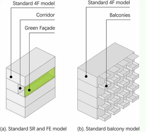
In the FE model, the leaf area density (LAD) of the foliage was estimated from 0.5–4.0 m² m⁻³, following the results from field measurements and literature surveys (Susorova, Azimi, and Stephens 2014; Lin et al. 2019; Gromke et al. 2015). According to Gromke et al. and Shashua et al. (Gromke et al. 2015; Shashua, Pearlmutter, and Erell 2009), the evaporation power (P_c) was estimated as P_c = 250 W m⁻³ for a plant with LAD = 1.0 m² m⁻³. As calculated in previous studies (Lin et al. 2019; Gromke et al. 2015), the P_c was set from 125–1000 W m⁻³ in the FE models. The study of foliage evaporation tents was performed to test the evaporation effects on temperature adjustments.

2.2.2. GFs layout typologies models

The standard balcony model (2.5 m × 3 m, L × W) was built based on the previous standard single CFD model (Figure 3(b)) (Lin et al. 2019). The normal width of a balcony is 1.5 m; however, this study expanded the width to evaluate the difference of the T_a and V_a behind the plant foliage. The previous study had conducted the standard simulations on different orientations (Lin et al. 2019). For this study, the main purpose was to develop a couple simulation method, thus, all models were simplified and only set to face south.

Seven cases of GF typologies on the standard balcony model and one unshaded model (UN) were built to test different layout strategies of GFs. GF typologies included the front, the side, the back, and the railing around the balcony. The front GF models were divided into three typologies: GFs in front of the balcony (Front-1, F1), GFs in front of the balcony with openings (Front-2, F2), and GFs with full shade (Front-all, FA). The side GF models were divided into two typologies: double side GFs (DS) and single side GFs (SS). Furthermore, the GF railing model (GR) and the GW model at the back side of the balconies were also defined for comparison. The models are listed in Table 3. The GF thicknesses were set at 0.3 m, using the field measurements as a guide.

Table 3. Definition and description of the balconies GF models.

Model name	Model description & photo	Model name	Model description & photo	Model name	Model description & photo
Un	Unshaded	F1	GFs in front of the balcony	F2	GFs in front of the balcony with openings
FA	GFs fully shaded	DS	Double side GFs	SS	Single side GFs
GR	GF Railings	GW	Green Wall

2.3. Setting of CFD simulations

2.3.1. The standard CFD model setting and the grid sensitivity test

The standard process of the CFD simulations had been validated on T_a and V_a in the previous study (Lin et al. 2019). The software of ANSYS Fluent (Version 16.0, 2014 ANSYS, Inc.) was employed to solve the aerodynamics problems (Gromke et al. 2015; Shashua, Pearlmutter, and Erell 2009; Shih et al. 1995; Fidaros et al. 2010; Richards and Hoxey 1993; López et al. 2012; Mercer 2009; Boulard and Wang 2002; Liu, Chen, and Black 1996; Sanz 2003). The solving model was the three-dimensional steady-state Reynolds-averaged Navier–Stokes (RANS) equation with the Boussinesq approximation for the thermal environment and the realizable k-ϵ turbulence model (Shih et al. 1995). The discrete ordinates (DO) model was employed in the radiation model to solve the solar ray-tracing calculations (Fidaros et al. 2010). The second-order scheme was applied in the mean flow, turbulence, and energy equations discretization. The SIMPLEC scheme was applied in the coupling calculation with pressure and velocity. The convergence criteria of the continuity, velocity, energy, and DO model were set to 10⁻⁶.

The computational domain of the standard model was 152 m × 108 m × 96 m. The grid sensitivity of the standard model had been tested with the minimum scale of 0.05 m, 0.1 m, 0.2 m, and 0.4 m, and the results confirmed that the differences of T_a and V_a of different grid scales were lower than 3%; therefore, in this study, the minimum hex grid size of 0.1 m on the central study building and the maximum size of 1.0 m was applied to the computational domain boundary. The total cell number of the standard model was 3,404,835 (Figures 4 and 5).

Figure 4. Scale and boundary settings of the study models.

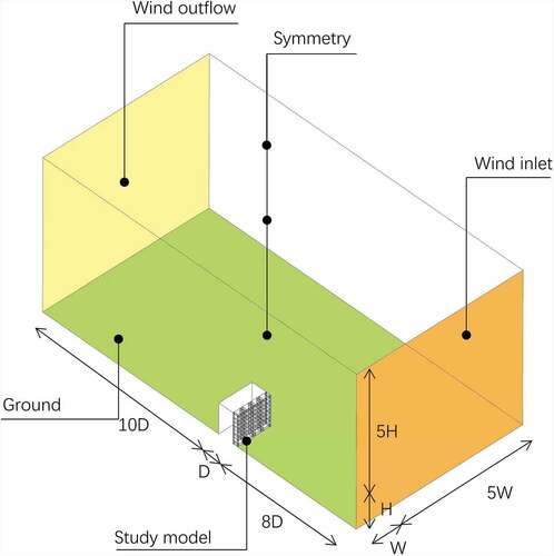
Figure 5. Detail of the test cells in the compute domains in the study models.

2.3.2. The boundary settings of the standard CFD model

In the boundary settings of the model, a vertical profile was defined at the wind-inlet boundary. The V_a, k, and ϵ of the neutrally stratified atmospheric boundary layer was set according to (Richards and Hoxey 1993)..

(1) $\begin{array}{c}{\mathrm{V}}_a\left(\mathrm{z}\right)=\frac{u_{\ast }}{k}ln\frac{z+z_0}{z_0}\end{array}$(1)

(2) $\begin{array}{c}\begin{array}{c}k\left(\mathrm{z}\right)=\frac{u_{\ast }^2}{\sqrt{C_u}}\end{array}\end{array}$(2)

(3) $\begin{array}{c}\epsilon \left(z\right)=\frac{u_{\ast }^3}{k\left(z+z_0\right)}\end{array}$(3)

where C_u = 0.09; z₀ = 0.5 m; V_a was set as 1.0 m s⁻¹ at a height of 10 m in the standard model.

Using the previous studies as a guide, the properties of the model boundaries of symmetry, outlet airflow, building walls, and the ground were set (Table 4) (Lin et al. 2019; Gromke et al. 2015; Richards and Hoxey 1993; Boulard and Wang 2002; Liu, Chen, and Black 1996; Sanz 2003). The setting of the building walls include thermal insulation and surface material layer is about 240–270 mm in hot-humid climate and about 300–350 mm in temperate climate, thus, it was simplified to defined as 300 mm in the simulation. Considering the simulation comparison was mainly focused on the different green façade models, thus, the multi-layer of the ground material was simplified to a same setting (Gromke et al. 2015).

Table 4. Boundary conditions of the standard model.

Property	Fluid	Building Walls	Ground	GF Foliage
Materials	Air	Concrete	Asphalt	Porous materials
Thickness (m)	−	0.3	10	0.3
$\rho$ (kg m^−3)	1.225	2000	1600	700
Specific heat capacity (J kg^−1 K^−1)	1006.43	900	300	2310
Thermal conductivity (W m K^−1)	0.0242	0.8	0.8	0.173
Viscosity	1.7894 × 10^−5	−	−	−
Absorption coefficient	0.19	0.9	0.9	0.75
Scattering coefficient	0	0	−10	0
Emissivity	0.9	0.7	0.95	0.983
Ts (°C)		20	10	−
Roughness height		0	0.05	−
Roughness constant		0	0.5	−

The GFs were defined as porous zones in the CFD simulation (López et al. 2012; Mercer 2009), whose transpiration cooling power (P_c) was estimated to be 500 W m⁻³ in previous studies (Lin et al. 2019; Gromke et al. 2015; Boulard and Wang 2002). The wind-induced effect of the GFs was defined with the momentum, k, and ϵ equations terms (Lin et al. 2019; Gromke et al. 2015; Boulard and Wang 2002)..

(4) $\begin{array}{c}{S}_{u_i}=-{\rho }_a{C}_{d}LAD{U}_i{V}_a\end{array}$(4)

(5) $\begin{array}{c}\begin{array}{c}{S}_k={\rho }_a{C}_{d}LAD\left({\beta }_p{V_a}^3-{\beta }_d{V}_a{k}_a\right)\end{array}\end{array}$(5)

(6) $\begin{array}{c}\begin{array}{c}{S}_{\epsilon }={\rho }_a{C}_{d}LAD\frac{\epsilon }{k}\left(C_{\epsilon 4}{\beta }_p{V_a}^3-C_{\epsilon 5}{\beta }_d{V}_a{k}_a\right)\end{array}\end{array}$(6)

where ${\rho }_a$ = 1.225 kg m⁻³; C_d = 0.2; ∆l = 0.3 m; β_p = 1.0; β_d = 5.1; k_a = 0.42; C_ε4 = C_ε5 = 0.9; LAD = 1 m² m⁻³ (LAD = LAI/∆l) following the definition in the previous studies (Lin et al. 2019; Gromke et al. 2015; Shashua, Pearlmutter, and Erell 2009; Shih et al. 1995; Sanz 2003).

2.4. Couple simulations

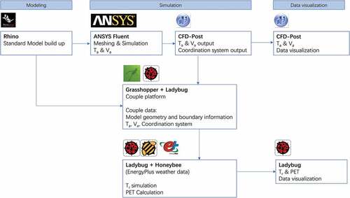
To evaluate the human thermal comfort indices, such as PET, more indices were input into the simulation, including the RH, the mean radiant temperature (T_r), and body characteristics of a human being, which were simulated in a series of algorithms using Ladybug tools (LB, Version 0.0.68) with Honeybee (HB, Version 0.0.65) (Sa 2021). LB is a collection of open-source applications and integrated workflows that support the analysis and improvement of the built environment’s performance and was developed based on Grasshopper ® (GH) (SB 2021) in the 3D modeling software Rhino® (RN, Version 6.0, Robert McNeel & Associates.) (SC 2021). HB connects GH to different simulation tools to construct the energy and daylight simulation.

The couple simulations with CFD and LB were based on the same building models and the same coordinate system, which supported the simulation data interaction in GH. In the Ansys software package, a post-processor software named CFD-post (in Ansys 16.0) supported the data of T_a and V_a, and exported the coordinate system data. The central parts of the simulation zone in CFD, including the building surface and the volumes of the balconies and GFs, were meshed with isometric grids with the same grid length of 0.1 m, which defined as the same grid size in LB and HB launching EP. Consequently, the data of T_a and V_a were read in LB, and the coordinate system was rebuilt in RN (Figure 6).

Figure 6. Couple simulation process.

For the simulation models, the balcony areas were defined as HBZones in LB and HB and exported into an OpenStudio® (OS, Version 3.1.0) (SD 2021) file for simulation using the software EnergyPlus^TM (EP, Version 8.8, Alliance for Sustainable Energy, LLC) (SE 2021). The GFs were defined as shading components of the HBZones with the transmittance being obtained from the field measurements. Consequently, an open-source weather date file (*.epw file) of Guangzhou, China, was collected from EP (SF 2021) and imported to create a specific site climate for the simulation.

We obtained the standard building model geometric parameters from RN, the indices of the building and environment surface temperatures (T_s), and sky view factor (SVF), and used these values for the simulation, using LB and HB, which launched EP on the environmental parameters. The computation of T_s was based on the baffle heat balance assumption that the baffle is sufficiently thin and has high conductivity so that it can be modeled using a single temperature (EnergyPlus™ Version 9.4.0 Documentation 2021). The T_s is determined by formulating a heat balance on a control volume that enclosed the baffle surface. According to (EnergyPlus™ Version 9.4.0 Documentation 2021), the heat balance on the baffle surface’s control volume is:

(7) $\begin{array}{c}{q}_{\alpha sol}^H+q_{LWR,Env}^H+q_{conv,Env}^H+q_{LWR,cav}^H+q_{conv,cav}^H=0\end{array}$(7)

The T_s is:

(8) $\begin{array}{c}{T}_s=\frac{\left(I_s\alpha +h_{co}{T}_a+h_{r,atm}{T}_a+h_{r,sky}{T}_{sky}+h_{r,gnd}{T}_a+h_{r,cav}{T}_{so}+h_{c,cav}{T}_{a,cav}\right)}{\left(h_{co}+h_{r,air}+h_{r,sky}+h_{r,gnd}+h_{r,cav}+h_{c,cav}\right)}\end{array}$(8)

Then, the SVF for each HBZone was calculated via reflection factor (RF) in the following equation (EnergyPlus™ Version 9.4.0 Documentation 2021):

(9) $\begin{array}{rl}& RF\left(R{S}_{num}\right)=\frac{1}{N_{rec}}\sum _1^{N_{rec}}\sum _{i=1}^{N_{ray}}Hi{t}_{obs,i}SV{F}_{obs,i}\\ & DifShadgRatioIsoSk{y}_{obs,i}{\rho }_{obs,i}cos\frac{a_i}{\pi }\end{array}$(9)

In the above equation, $DifShadgRatioIsoSk{y}_{obs,i}$ = (obstructed sky irradiance on obstruction)/(unobstructed sky irradiance on obstruction). $SV{F}_{obs,i}DifShadgRatioIsoSk{y}_{obs,i}$ is the sky irradiance at the hit point divided by the horizontal sky irradiance when considering the shadow of the sky diffuse radiation on the obstruction caused by other reflections. The irradiance at one hit point by the reflection of sky radiation from the ground or from other obstructions is not considered.

Basing on the calculation above, both indices of T_s and SVF were imported to calculate the T_r with the HB algorithm. According to the ISO 7726 (International Organization for Standardization. Available online 2021), the T_r could be calculated from the surrounding surface weighted by the surface emissivity:

(10) $\begin{array}{c}{T}_r=\frac{\sum {\epsilon }_i{F}_i{\left(T_s\right)}^4}{\sum {\epsilon }_i{F}_i}\end{array}$(10)

Coupling with the data files of T_r, V_a, T_a, and a group of preset values including RH (70%), obtained from the average value in the field measurements and the parameters of a human being (Table 5), the PET was calculated via the algorithm “ThermalComfortIndices” in LB basing on the PET calculation method according to the Munich Energy–balance Model for Individuals (MEMI) (Höppe 1999; Ng and Ren 2015).

Table 5. Preset values of a human being used in our study (Niu et al. 2015; Jin, Zhang, and Zhang 2017).

Characters	Preset value
Age	30
Sex	male
Height	175 mm
Weight	75 kg
Body position	standing
Clothing insulation	0.57 clo*
Clothing albedo	37 %
Metabolic rate	2.0

*0.57 clo for short-sleeved shirt with trousers.

2.5. Visualization of the simulations results

Visualizations of the CFD and coupling simulation results on the building model yield a clearer picture of the distribution of different thermal environmental indices. In this study, the CFD results (V_a and T_a) were visualized in CFD-post, and the coupling simulations results (T_r and PET) were visualized in HB and RN (Figure 6). The simulation results could be applied to different building floorplans and sections to obtain a much more comprehensive understanding of the effects of the GFs.

3. Results

3.1. Results of field measurements

3.1.1. Solar radiation results

Results of the measurements between the shaded and unshaded area for ten days in June 2019 revealed that the average reduction of the G_a was 73.29% (Table 6). The field measurements conducted over 10 days sufficiently captured different weather characteristics. The G_a of the unshaded area varied from 53.27 W m⁻² to 403.00 W m⁻² on different days due to weather changes; the shaded area stayed below 150 W m⁻² in the measurement period Figure 7.

Figure 7. Results of G_a measurements compared to GF shading (GF) and unshaded (UN) areas in ten days.

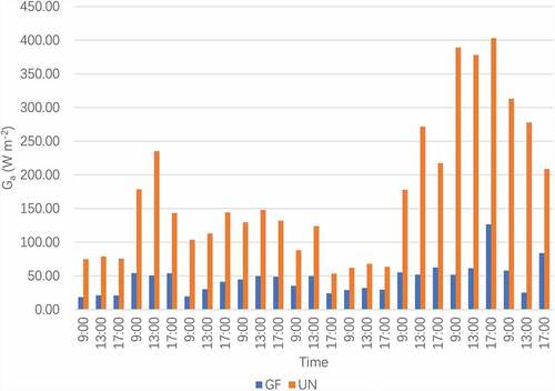
Table 6. Results of G_a measurements compared to GF and unshaded (UN) areas.

Indices	Ga of GF (W m^−2)	Ga of UN (W m^−2)	Shading ratio (%)
Ave. Ga	43.14	162.08	73.39
Max. Ga	126.45	403.00	68.62
Min. Ga	18.34	53.37	65.64

These results show that the foliage layer presented a significant and stable shading effect and showed significant potential to reduce building energy consumption. Compared to the previous studies, the result of the G_a reduction in this study was higher than Jim’s measurement of 67.9% (Jim 2015b) but close to the result of 76.7% from Šuklje et al. (Šuklje, Medved, and Arkar 2016; Šuklje et al. 2019).

3.1.2. Foliage parameters results

The measurements of the five GF units are shown in Figure 8. The LAI was 1.56–3.61 and the FCR was 49.74–92.88%. Correlation analysis was performed on two group data and showed that two parameters had a high correlation (R² > 0.8). These results imply that both methods could determine the coverage capacity of a GF’s foliage layer.

Figure 8. Examples of figure and pixel analysis for the FCR calculation and comparison with LAI values (Fig, figure of the climbing plants; Pix, pixel analysis of the climbing plants).

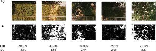
Compared to the results from previous studies, Lee & Jim estimated that the LAI of the scatter foliage of a climbing plant is 0.24 (Köppen 2011); Susorova et al. estimated that the LAI of much denser foliage is 2.0 (Susorova, Azimi, and Stephens 2014). In our study, the foliage thickness of the climbing plants ranged between 0.4 and 0.5 m, and had a significantly increased LAI value. Sulaiman et al. had investigated three climbing plants to determine the FCR value via measurements and found that the FCR values were in the range of 69.4% – 86.5% (Sulaiman, Jamil, and Zain 2013; Azhar Mat Sulaiman et al. 012025); however, few studies have compared both parameters for the same plants. In our study, we provide a new perspective to evaluate the coverage ratio of a GF.

Regarding the GF simulations, the FCR value was defined as the transmittance of a shading component in LB and HB, and the LAI value was used to calculate the GF’s foliage density with the foliage layer thickness computing the C_d and the P_c in CFD simulations. Both parameters were shifted to the definition of the GF model in the following simulations.

3.2. Results of CFD Simulations on the standard model

3.2.1. Simulations of SR Model

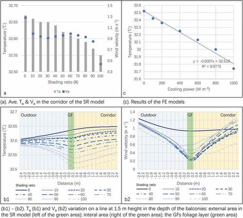
In the SR model, SR was defined with ten levels to shade the corridor. The results revealed that T_a and V_a decreased when the SR increased. The Ave. T_a and V_a of the corridor were reduced by 0.05–0.2°C and 0.15–0.6 m s⁻¹ at different SR levels (Figure 9(a)). A visualization of the T_a and V_a distribution at the section of the standard model was added. The data were taken as a series of points in a line along the depth of the balconies at the height of 1.5 m. The results in the corridor section provide a much clearer understanding of the adjusting effects on T_a and V_a, showing that both indices were reduced more when there was a smaller distance to the GFs (Figure 9 (b1 – b2)). Though the changes of the T_a were simulated at a low level, the simulations revealed that the shading and wind-induced effects of the GFs strengthened when the SR increased.

Figure 9. Results of the SR and FE models in the CFD simulations.

3.2.2. Simulations of FE Models

The FE models simulated the P_c value from 125 to 1000 W m⁻³ for the LAD value from 0.5 to 4.0 m² m⁻³ (Gromke et al. 2015) a model without FE was added to compare. The results reveal that the Ave. T_a of the corridor decreased with the increase of the P_c. The Max. T_a was reduced by 0.75°C when the P_c was set to 1000 W m⁻³ in the experiments (Figure 9(c)). In the correlation analysis, the P_c and T_a presented a negative correlation (R² > 0.9) in the experiment, implying that the increase in the P_c, as well as the density of the foliage layer, could improve thermal comfort in the corridor.

3.3. Results of CFD simulations on the balcony models

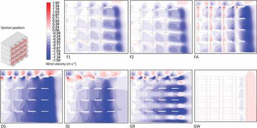
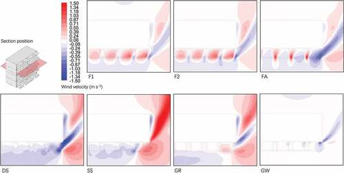
The balcony models were first simulated in Ansys Fluent 16.0 to obtain the T_a and V_a results. The V_a results showed that the model DS, SS, GR, and FA provided much more significant effects on the wind environment and the Ave. V_a reduction was 0.77 m s⁻¹, 0.50 m s⁻¹, 0.29 m s⁻¹, and 0.20 m s⁻¹ (Table 7). Compared to the UN model, the DS model showed that Ave. T_a was reduced to 0.2°C, whereas the T_a reduction of the other models was lower than 0.1°C (Table 7). A section was added to analyze the V_a and T_a distribution inside and outside the balconies’ area. The T_a data showed little difference between the cases with a temperature of 0.1°C. Wind static pressure (P_r) showed a much more significant pressure drop in the balconies’ areas, especially in FA, F2, F1, and GR. Thus, the V_a of FA, F2, F1, and GR also showed much more reduction behind the GFs. The section data allows for a clearer description of the wind-induced effect of the GFs (Figure 10).To provide a deeper analysis of T_a and V_a differences in the corridor space, the contour maps were created using the CFD-Post software, and the resulting case data were input into the same coordinate system to compare to the UN model. Three sections were defined in CFD-Post to demonstrate the horizontal and vertical distributions of the data of T_a and V_a.

Figure 10. T_a, V_a, and P_r distribution on a line at 1.5 m height in the depth of the balcony.

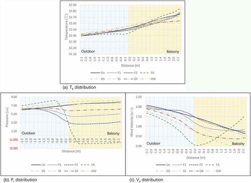
Table 7. Ave. T_a and V_a at a surface height of 1.5 m on the balconies.

	GF Typologies
Indices	UN	DS	SS	F1	F2	FA	GR	GW
Ta (°C)	33.00	32.80	32.97	32.97	32.95	32.99	32.94	32.98
Va (m s^−1)	0.90	0.13	0.40	0.88	0.88	0.70	0.61	0.80

In the front-vertical section (Figures 11 and 12), the models of DS, SS, GR, and FA showed clearer effects on V_a, especially on the bottom and the edge (the right side of the model) areas of the model because of the air turbulence variation at the building corner. T_a was reduced slightly in the models of FA, DS, and GR in the middle of the balconies that implied the GFs may improve the thermal comfort better in these cases. T_a results also showed that the top floor exposing to the solar radiation may be overheated and need much more shading or vegetation devices. Comparably, the GW model presented the lowest effect on both indices.

Figure 11. T_a simulation results: Distribution on the front-vertical section (difference of the models subtracting to the UN model. Red area – results higher than the UN model; blue area – results lower than the UN model).

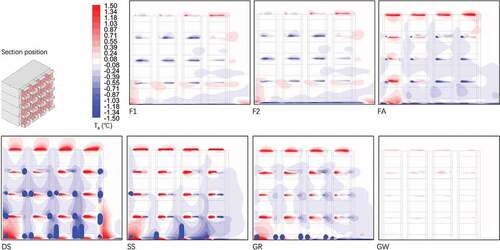
Figure 12. V_a simulation results. Distribution on the front-vertical section (difference of the models subtracting to the UN model. Red area – results higher than the UN model; blue area – results lower than the UN model).

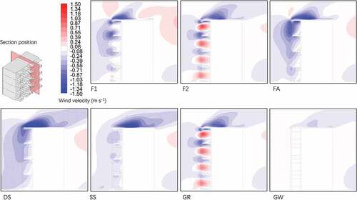
In the cross-vertical section (Figures 13 and 14), the contour maps showed the GFs’ effects on the thermal environment in the middle of the balconies. The changes in T_a mainly occurred in the first to the third floor in models of DS, FA, and GR, respectively, in which V_a mainly appeared in the edge areas in most models except GW. We noticed that the GF reduced the T_a at 0.5°C at a distance of 1 m on the ground in front of the balconies, revealing GFs’ optimization effect on the thermal environment of the surrounding area. On the other hand, the reduction of V_a around the GFs implied that the building design may need to concern the negative effects of GFs on natural cross ventilation.

Figure 13. T_a simulation results. Distribution on the cross-vertical section (difference of the models subtracting to the UN model. Red area – results higher than the UN model; blue area – results lower than the UN model).

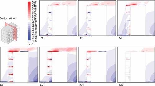
Figure 14. V_a simulation results. Distribution on the cross-vertical section (difference of the models subtracting to the UN model. Red area – results higher than the UN model; blue area – results lower than the UN model).

In the horizontal section on the third floor (h = 7.5 m, Figures 15 and 16), the contour maps also showed the GF shading and wind-induced effects on the T_a and V_a, especially in DS, GR, and FA models. The GW model presented the lowest effect on T_a and V_a at a distance of 0.5 m. We also found that the T_a around the building was reduced due to the air turbulence variation. It also implied that the potential of GFs’ effect on thermal comfort may not only existed on the balconies but also in the surrounding environment.

Figure 15. T_a simulation results. Distribution on the horizontal section (difference of the models subtracting to the UN model. Red area – results higher than the UN model; blue area – results lower than the UN model).

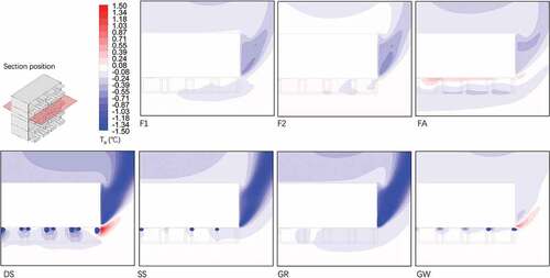
Figure 16. V_a simulation results. Distribution on the horizontal section (difference of the models subtracting to the UN model. Red area – results higher than the UN model; blue area – results lower than the UN model).

3.4. Results of T_r on the balcony models

Once we performed the CFD simulations for the balcony models, we performed simulations in the LB and HB with the T_a and V_a data and a coordinate system.

In the T_r comparison, the results revealed that the reduction of T_r in FA, F1, F2, DS, GR, SS, and GW models was 7°C, 5.5°C, 3.7°C, 3.5°C, 2.1°C, 2.0°C, and 0.5°C, respectively (Table 8). These results imply that the GFs, as the shading component on the front side, provided a suitable reduction of solar radiation. Furthermore, when comparing the T_r results of DS and SS models, the results show that increasing the foliage layer area would positively affect the reduction of solar radiation. The GW model results also show a reduced Ave. T_r by 0.5°C and GW also provided regulation of indirect radiation from vertical surfaces.

Table 8. Ave. T_r, and PET at a surface height of 1.5 m on the balconies.

	GF Typology
Indices	Un	F1	F2	FA	DS	SS	GR	GW
Tr (°C)
Ave	39.83	34.31	36.17	32.90	36.37	37.80	37.78	39.32
Max	41.88	38.16	39.63	36.65	39.90	41.79	41.03	41.66
Min	38.80	31.12	30.99	31.64	31.44	32.52	36.38	38.13
PET (°C)
Ave	36.08	33.34	34.16	32.92	34.73	35.55	35.26	35.80
Max	37.05	34.55	35.53	34.05	37.26	37.41	36.71	36.87
Min	34.89	31.32	31.26	32.43	29.89	30.22	33.87	34.49

3.5. Results of the coupling simulations on PET

The results of PET were similar to T_r and the reduction in PET in the FA, F1, F2, DS, GR, SS, and GW models was 3.2°C, 2.7°C, 1.9°C, 1.4°C, 0.8°C, 0.6°C, and 0.3°C, respectively (Table 8). In the PET category, thermal comfort was considered to be between the “moderate heat pressure” and “strong heat pressure” level for all models. The PET results at the height of 1.5 m revealed that the GFs of the FA, F1, and F2 models showed much more significant effects on thermal comfort (Figure 17). The adjustment of PET in other models appeared to limit the areas with a 0.5 m distance, which implied that the layout of the GFs would influence the optimization of the thermal comfort as well.

Figure 17. PET distribution results on a surface of 1.5 m on the third floor (h = 7.5 m) in the balcony models.

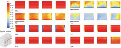
The PET and T_r results revealed that the HCT in the balcony models was mainly affected by solar radiation, implying that the shading effect would be important in GF applications.

4. Discussion and limitations

4.1. Measurement and prediction indices for SR of GFs

SR was a key factor for the shading effect of GFs on thermal environmental adjustment; however, it is not easy to measure or predict the SR of a plant that grows vertically. Several factors limit the reliability of field measurements. Firstly, GFs include different species of climbing plants with various growing mechanisms, such as tendrils twining, stems and leaves twining, thorns hooking, and roots adsorbing (Jim 2015b; Herron et al. 2007; Burnham 2021). For the climbing plants adsorbing on the wall surface, there is no space between a foliage layer and a wall to install the measurement equipment. Secondly, some field investigations on GWs have shown that GWs installed on the exterior space of high-rise buildings are difficult to maintain due to problems of accessibility, structural stability, and material durability (Chew, Conejos, and Azril 2019). The long-term monitoring equipment of SR integrating with the façade system is often lacking. Thirdly, there is a lack of synergistic controls on thermal environmental adjustment methods with the variation of GF foliage properties and GF monitoring is normally absent.

In this study, we compared two methods that determine the foliage parameter measurements of GFs to provide a simpler method for evaluating the foliage layer using digital photos, which could be collected with simple cameras. We hope that this method supports a better understanding and maintenance of GFs. The high correlation of the two methods validated the method of photo-pixel post-processing using solar radiation measurements. This simpler image collection method could be used for daily maintenance in many different GFs, even using a user’s mobile phone. To measure a GF on a high-rise building, a façade-cleaning machine or an uncrewed aerial vehicle could support the collection of images. Future research is still required to test foliage images and color pixel recognition with different plant species, in different seasons, and to distinguish between leaves and stems.

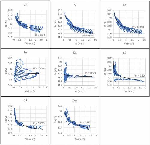
4.2. Regression analysis of T_a and V_a in CFD simulations

The CFD simulation in this study was based on the coupling computation with the air and thermal transmission. The GFs were simulated with a definition of a porous zone, which accounted for the wind-induced and evaporation cooling effects. T_a and V_a are two main indices useful for discussing the results; a regression analysis was also performed. The analysis revealed that the two indices presented a logarithmic relationship, and the R² was higher than 0.7 in most models (Figure 18). With an increase in V_a, the T_a reduced due to the cooling effect of the GFs; however, in the FA and DS models, the correlation with the two indices was not obvious. Considering the wind-induced effect and the higher SR of these two models, the V_a in the above two models had been reduced to a low level such that the distribution of T_a in different ranges became dispersive.

Figure 18. Regression analysis with T_a and V_a in CFD simulations.

In this study, we mainly focused on the balcony areas, which were defined as one typology of transitional spaces; further studies should include other urban environments to investigate the previously mentioned indices.

4.3. Correlation and regression analysis of thermal indices with PET

In this study, we conducted a coupled simulation with CFD and LB with HB launching EP. The relationship between the indices is required for the analysis of the different effects on HTC.

The correlation analysis of T_r and PET revealed that the correlation index (CI) of F1, F2, FA, and DS models was higher than 0.6, and for T_a and PET, it was higher than 0.7 in the Un and GW models. The CI of V_a and PET was calculated in the minus zone and revealed that V_a harmed thermal comfort regulation; however, only the absolute value of CI of the Un, GR, and GW models was higher than 0.7 (Table 9). In the regression analysis, the R² of T_r and PET was higher than 0.6 in F1 and DS models, for T_a and PET, it was higher than 0.5 in the Un and GW models, and for V_a and PET, it was higher than 0.7 in Un and GW models (Figures 19, 20, and 21).

Figure 19. Regression analysis with T_r and PET in the coupled simulations.

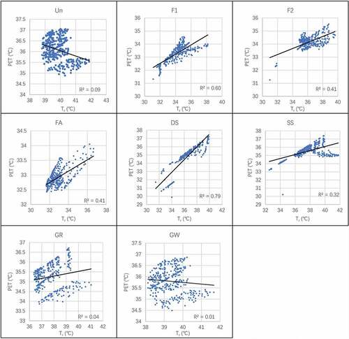
Figure 20. Regression analysis with T_a and PET in the coupled simulations.

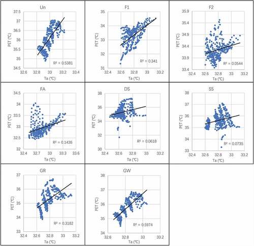
Figure 21. Regression analysis with V_a and PET in the coupled simulations.

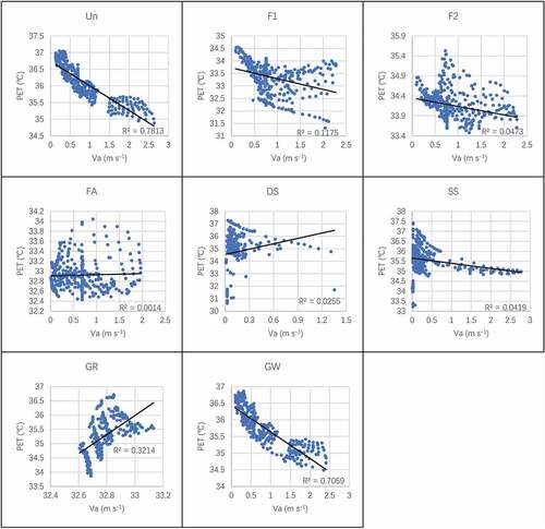
Table 9. Correlation analysis of indices with PET.

Indices	Correlation index
	Un	F1	F2	FA	DS	SS	GR	GW
Tr & PET	–0.30	0.77	0.64	0.64	0.89	0.56	0.19	–0.10
Ta & PET	0.73	0.58	0.23	0.38	0.25	0.27	0.56	0.77
Va & PET	–0.88	–0.34	–0.22	0.04	0.16	–0.20	–0.72	–0.84

Comparing the CI and R² of different thermal indices with PET, the T_r yielded a much more obvious effect on thermal comfort, which implies that the shading effect contributes a stronger influence on thermal comfort regulation, which was discussed in previous field measurements in different climates (Coma et al. 2017; Köppen 2011; Lin, Xiao, and Musso 012006; Lin et al. 2019; Jim 2015b). One could notice that different layouts of GFs also showed different impacts on thermal comfort regulation. The front-side layout (F1, F2, and FA) yielded better effects on the shading. Both regression analyses revealed that the GFs affected T_a and V_a in CFD simulations but contributed little effects on PET in the coupled simulation.

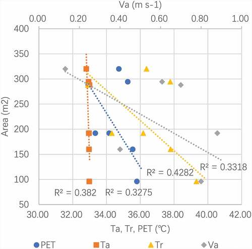
4.4. Regression analysis of foliage layer area with thermal indices

Considering that the foliage areas of the different GF models are different, an additional regression analysis was performed on foliage areas with T_a, V_a, T_r, and PET. The results revealed that the R² was between 0.3–0.5 (Figure 22), implying that the effects of the foliage area were weak. The layout and the shading method of the GFs may present a much more important effect on thermal comfort, as noted in the discussion above.

Figure 22. Regression analysis with foliage area and different thermal environment indices in the coupled simulations.

4.5. Couple method for thermal comfort simulations

More and more couple simulations are conducted with CFD and various building energy simulation (BES) methods (Pandey, Banerjee, and Sharma 2021) for building environment and energy research. Internal and external approaches are the two main methods of couple simulation. The internal method requires that the simulation be conducted in the same software and model; however, the external method usually uses different CFD and BES software but shares the same model and boundary information, such as the climate, the building envelope, and the building scale and coordination system (Pandey, Banerjee, and Sharma 2021). Most studies with couple methods are focused on a better prediction of building energy considering the outdoor and indoor air and heat transmission (Tian et al. 2018). Most studies investigated the thermal environments of indoor environments with various methods to transfer boundary conditions from EP to CFD tools (Tian et al. 2018; Shan et al. 2020).

In this study, we followed the external couple method and introduced the open-source LB and HB algorithm to transfer the data from CFD simulation, launch the EP for T_r simulation, and calculate the PET. We must use the same model, the same computation grid, the same coordination system, and the same boundary conditions of two series of simulations for data transportation and calculation for the couple method to work properly.

Some aspects may be improved in future studies following the couple method development. This method assumed that the thermal environment was steady and each simulation was only calculated at a specific time; in future investigations, a continuous simulation method would be useful (Pandey, Banerjee, and Sharma 2021). The simulation data transfer and the models and boundary condition settings were manually conducted in this study and could be improved via automation. The inclusion of building energy assessment could also be beneficial for the couple simulation.

4.6. Limitations of GF model settings

Our model only used a standard balcony model with one orientation and one specific time to compare different shading strategies with the method of couple simulation, which could be studied in the border area of models. In the building scale, different aspects such as indoor environment, outdoor environment, and urban canyon may be considered in further studies to evaluate the effects of GFs. In the boundary condition settings, the building orientation and weather conditions, such as outdoor T_a, V_a, RH, and solar radiation, may be defined and tested following the local climate data in applications. In the definition of GF, this study only tested a standard setting of the foliage layer, however, the foliage of different plants and in different seasons would be different and need much more specific definition in research and applications. Furthermore, more time steps for the simulation may be useful for continuous climate data but require more computation resources, such as more CPU cores and increased time to process. In this study, we constructed a working process that could support future studies in the future.

5. Conclusions

This study extends the previous study on thermal comfort assessment in a transitional space in a hot and humid climate area. The main purpose of this study was to develop a couple method on HTC simulations that involved GF SR evaluation, related parameter testing, and a working process construction. The main findings and results are as follows:

• In the GFs’ shading effects evaluation, Ave. G_a was reduced by 73.29% in field measurements.

• In the field measurements of the GFs’ foliage layer, the LAI range was 1.56 - 3.61 and the FCR range was 49.74 - 92.88%. Both indices presented a high correlation (R² > 0.8).

• Two CFD simulations on a standard model were conducted on the SR and FE simulations. In the SR model, the Ave. T_a and V_a of the corridor were reduced by 0.05 - 0.2°C and 0.15 - 0.6 m s⁻¹, respectively, in the SR range of 10 - 100%. In the FE model, the Ave. T_a of the corridor decreased with the increase of the P_c and the Max. T_a was reduced by 0.75°C when P_c was 1000 W m⁻³.

• In the CFD simulations on the balcony model, the Ave. V_a was reduced by 0.77 m s⁻¹, 0.50 m s⁻¹, 0.29 m s⁻¹, 0.20 m s⁻¹ in the DS, SS, GR, and FA models, respectively, and the Ave. T_a was reduced by 0.2°C in the GF models.

• In the T_r simulations, the reduction of T_r in FA, F1, F2, DS, GR, SS, and GW models was 7°C, 5.5°C, 3.7°C, 3.5°C, 2.1°C, 2.0°C, and 0.5°C, respectively.

• In the PET calculations, the reduction of PET in FA, F1, F2, DS, GR, SS, and GW models was 3.2°C, 2.7°C, 1.9°C, 1.4°C, 0.8°C, 0.6°C, and 0.3°C, respectively.

In conclusion, the shading effect should be recognized as a key effect on thermal comfort in a transitional space, and the distribution of GF to provide shading on the front side will improve thermal comfort. In this study, the method of couple simulation with CFD and thermal comfort calculation via LB and HB was developed and could support the architectural and landscape design integrating with the GFs.

Nomenclature and abbreviations

Cd	Leaf drag coefficient	$q_{asol}^{{ }^{\prime \prime }}$	Absorbed direct and diffuse solar (short wavelength) radiation heat flux (W m^−2)
Cε4	Empirical coefficient of ε4	$q_{conv,cav}^{{ }^{\prime \prime }}$	Surface convection flux exchange with cavity air (W m^−2), “conv, cav” denotes to the convection flux and the cavity air
Cε5	Empirical coefficient of ε5	$q_{conv,Env}^{{ }^{\prime \prime }}$	Surface convection flux exchange with outside air (W m^−2), “conv, Env” denotes to the convection flux and the outside air
CI	Correlation index	$q_{gnd}^{{ }^{\prime \prime }}$	Ground surface longwave radiation flux (W m^−2)
Cu	Empirical drag coefficient	$q_{LWR}^{{ }^{\prime \prime }}$	Exterior surface longwave radiation flux (W m^−2)
${\mathrm{F}}_{\mathrm{a}\mathrm{i}\mathrm{r}}$	View factor of wall surface to air surface temperature	$q_{LWR,cav}^{{ }^{\prime \prime }}$	Net longwave (thermal) radiation flux exchange with the outside face of the underlying surface(s) (W m^−2), “LWR, cav” denotes to the net longwave radiation and the outside face
${\mathrm{F}}_{\mathrm{g}\mathrm{n}\mathrm{d}}$	View factor of wall surface to ground surface temperature	$q_{LWR,Env}^{{ }^{\prime \prime }}$	Net longwave (thermal) radiation flux exchange with the air and surroundings (W m^−2), “LWR, Env” denotes to the net longwave radiation and the air and surroudings
${\mathrm{F}}_{\mathrm{i}}$	Angle factor between person and surface	$q_{sky}^{{ }^{\prime \prime }}$	Sky surface longwave radiation flux (W m^−2)
FCR	Foliage coverage ratio (%)	SVF	Sky view factor
${\mathrm{G}}_{\mathrm{a}}$	Global irradiation (W m^−2)	$\mathrm{S}\mathrm{V}{\mathrm{F}}_{\mathrm{o}\mathrm{b}\mathrm{s},\mathrm{i}}$	Unobstructed sky view factor of the obstruction $=\left(1+costil{t}_{obs}\right)/2$, “obs, i” denotes the obstruction hit by ray i
$h_{co}$	Convection coefficient for the outdoor environment (W m^−2 K^−1)	$\mathrm{R}\mathrm{F}$	Reflection factor
$h_{c,cav}$	Convection coefficient for the surfaces facing the plenum (W m^−2 K^−1), “c, cav” denotes the convection coefficient	RH	Relative humidity (%)
$h_{r,atm}$	Linearized radiation coefficient for the surrounding atmosphere (W m^−2 K^−1), “r, atm” denotes the radiation for the surrounding atmosphere	$\mathrm{R}{\mathrm{S}}_{\mathrm{n}\mathrm{u}\mathrm{m}}$	The receiving surface number
$h_{r,gnd}$	Linearized radiation coefficient for the ground (W m^−2 K^−1), “r, gnd” denotes the radiation for the ground	${\mathrm{T}}_{\mathrm{a}}$	Dry bulb air temperature (°C)
$h_{r,sky}$	Linearized radiation coefficient for the sky (W m^−2 K^−1), “r, sky” denotes the radiation for the sky	${\mathrm{T}}_{\mathrm{a},\mathrm{c}\mathrm{a}\mathrm{v}}$	Dry bulb temperature for air in the cavity (°C), “a, cav” denotes the air and the cavity
$\mathrm{H}\mathrm{i}{\mathrm{t}}_{\mathrm{o}\mathrm{b}\mathrm{s},\mathrm{i}}$	Number of the ray(s) an obstruction, “obs, i” denotes the obstruction hit by ray i	${\mathrm{T}}_{\mathrm{a}\mathrm{i}\mathrm{r}}$	Air surface temperature (°C)
${\mathrm{I}}_{\mathrm{s}}$	Incident solar radiation of all types (W m^−2)	${\mathrm{T}}_{\mathrm{g}}$	Globe temperature (°C)
k	Turbulence kinetic energy (m^2 s^−2)	${\mathrm{T}}_{\mathrm{g}\mathrm{n}\mathrm{d}}$	Ground surface temperature (K)
ka	van Karman constant	Ts	Surface temperature (K)
∆l	thickness of the foliage layer (m)	${\mathrm{T}}_{\mathrm{s}\mathrm{k}\mathrm{y}}$	Sky surface temperature (K)
LAI	Leaf area index	${\mathrm{T}}_{\mathrm{s}\mathrm{o}}$	Temperature of the outside face of the underlying heat transfer surface (°C)
LAD	Leaf area density (m^2 m^−3)	${\mathrm{T}}_{\mathrm{r}}$	Mean radiant temperature (°C)
${\mathrm{N}}_{\mathrm{r}\mathrm{e}\mathrm{c}}$	The number of receiving points	Ui	Velocity component of direction i (°C)
Pc	Cooling power of the foliage layer (W m^−3)	$u_{\ast }$	Friction velocity (m s^−1)
Pr	Static pressure (Pa)	${\mathrm{V}}_{\mathrm{a}}$	Wind velocity (m s^−1)
PET	Physiological equivalent temperature (°C)	z	Vertical position above ground (m)
$q_{air}^{{ }^{\prime \prime }}$	Air surface longwave radiation flux (W m^−2)	z0	Aerodynamic roughness length of the terrain windward of the computational domain (m)
Greek symbols
βd	Coefficient that accounts for short-circuiting of the eddy cascade	${\epsilon }_i$	Emissivity of the surface i
βp	Fraction of mean kinetic energy	ρ	Density (kg m^−3)
		ρa	Density of air (kg m^−3)
ɛ	Turbulence dissipation rate (m^2 s^−3)	$\sigma$	Stefan-Boltzmann constant (W m^−2 K^−4)
Abbreviation
BES	Building energy simulation	HTC	Human thermal comfort
CFD	Computational Fluid Dynamics	KCC	Köppen climate classification
DO	Discrete ordinates	LB	Ladybug tools
EP	EnergyPlus^TM	MEMI	Munich Energy-balance Model for Individuals
FE	Foliage evaporation	RANS	Reynolds-averaged Navier–Stokes
GF	Green facade	RN	Rhino®
GI	Green infrastructure	SR	Shading ratio
GR	Green roof	UGI	Urban green infrastructure
GW	Green wall	UHI	Urban heat island
HB	Honeybee	VG	Vertical green

Natural Science Foundation of Guangdong Province (2021A1515012387), Guangzhou Greening Company (GZLC-G202103)

Disclosure statement

No potential conflict of interest was reported by the author(s).

Additional information

Funding

This work was supported by the National Natural Science Foundation of China [52078214]; State Key Laboratory of Subtropical Building Science [2021ZB04].Natural Science Foundation of Guangdong Province (2021A1515012387), Guangzhou Greening Company (GZLC-G202103)

References

- 1964 Façade Planting [n]. 2010. Encyclopedic Dictionary of Landscape and Urban Planning, edited by Evert, K.-J., Ballard, E. B., Elsworth, D. J., Oquiñena, I., Schmerber, J.-M., Stipe, R. E., Berlin, Heidelberg, Germany: Springer Berlin Heidelberg. pp 323. doi: 10.1007/978-3-540-76435-9_4428.
- Aflaki, A., M. Mirnezhad, A. Ghaffarianhoseini, A. Ghaffarianhoseini, H. Omrany, Z.-H. Wang, and H. Akbari. 2017. “Urban Heat Island Mitigation Strategies: A State-of-the-Art Review on Kuala Lumpur, Singapore and Hong Kong.” Cities 62: 131–145. doi:10.1016/j.cities.2016.09.003.
- Azhar Mat Sulaiman, M. K., M. F. Shahidan, M. Jamil, and M. F. Mohd Zain. 2018. “Percentage Coverage of Tropical Climbing Plants of Green Facade.” IOP Conference Series: Materials Science and Engineering (401). 012025. doi:10.1088/1757-899X/401/1/012025.
- Boulard, T., and S. Wang. 2002. “Experimental Numerical Studies on the Heterogeneity of Crop Transpiration in a Plastic Tunnel.” Computers and Electronics in Agriculture 34: 173–190. doi:10.1016/S0168-1699(01)00186-7.
- Burnham, A. “Project of R. J.; Michigan, U. Of. CLIMBERS | Censusing Lianas in Mesic Biomes of Eastern RegionS.” Accessed July 10 2021. (http://climbers.lsa.umich.edu
- Casadesús, J., and D. Villegas. 2014. “Conventional Digital Cameras as a Tool for Assessing Leaf Area Index and Biomass for Cereal Breeding: Conventional Digital Cameras for Cereal Breeding.” Journal of Integrative Plant Biology 56 (1): 7–14. doi:10.1111/jipb.12117.
- Chew, M. Y. L., S. Conejos, and F. H. B. Azril. 2019. “Design for Maintainability of High-Rise Vertical Green Facades.” Building Research & Information 47 (4): 453–467. doi:10.1080/09613218.2018.1440716.
- China Meteorological Administration (in Chinese). Accessed July 10 2021. http://www.cma.gov.cn/en2014/
- Chun, C., A. Kwok, and A. Tamura. 2004. “Thermal Comfort in Transitional spaces—basic Concepts: Literature Review and Trial Measurement.” Building and Environment 39 (10): 1187–1192. doi:10.1016/j.buildenv.2004.02.003.
- Chun, C., and A. Tamura. 2005. “Thermal Comfort in Urban Transitional Spaces.” Building and Environment 40 (5): 633–639. doi:10.1016/j.buildenv.2004.08.001.
- Coma, J., G. Pérez, A. de Gracia, S. Burés, M. Urrestarazu, and L. F. Cabeza. 2017. “Vertical Greenery Systems for Energy Savings in Buildings: A Comparative Study between Green Walls and Green Facades.” Building and Environment 111: 228–237. doi:10.1016/j.buildenv.2016.11.014.
- EnergyPlus™ Version 9.4.0 Documentation. Accessed July 10 2021. (https://energyplus.net/documentation
- Fidaros, D. K., C. A. Baxevanou, T. Bartzanas, and C. Kittas. 2010. “Numerical Simulation of Thermal Behavior of a Ventilated Arc Greenhouse during a Solar Day.” Renewable Energy 35 (7): 1380–1386. doi:10.1016/j.renene.2009.11.013.
- Gromke, C., B. Blocken, W. Janssen, B. Merema, T. van Hooff, and H. Timmermans. 2015. “CFD Analysis of Transpirational Cooling by Vegetation: Case Study for Specific Meteorological Conditions during a Heat Wave in Arnhem, Netherlands.” Building and Environment 83: 11–26. doi:10.1016/j.buildenv.2014.04.022.
- Herron, P. M., C. T. Martine, A. M. Latimer, and S. A. Leicht‐Young. 2007. “Invasive Plants and Their Ecological Strategies: Prediction and Explanation of Woody Plant Invasion in New England.” Diversity and Distributions 13 (5): 633–644. doi:10.1111/j.1472-4642.2007.00381.x.
- Höppe, P. 1999. “The Physiological Equivalent Temperature - a Universal Index for the Biometeorological Assessment of the Thermal Environment.” International Journal of Biometeorology 43 (2): 71–75. doi:10.1007/s004840050118.
- Hunt, E. R., P. C. Doraiswamy, J. E. McMurtrey, C. S. T. Daughtry, E. M. Perry, and B. Akhmedov. 2013. “A Visible Band Index for Remote Sensing Leaf Chlorophyll Content at the Canopy Scale.” International Journal of Applied Earth Observation and Geoinformation 21: 103–112. doi:10.1016/j.jag.2012.07.020.
- International Organization for Standardization. Accessed July 10 2021. https://www.iso.org/standard/14561.html
- Isnard, S., and W. K. Silk. 2009. “Moving with Climbing Plants from Charles Darwin’s Time into the 21st Century.” American Journal of Botany 96 (7): 1205–1221. doi:10.3732/ajb.0900045.
- Jim, C. Y. 2015a. “Thermal Performance of Climber Green Walls: Effects of Solar Irradiance and Orientation.” Applied Energy 154: 631–643. doi:10.1016/j.apenergy.2015.05.077.
- Jim, C. Y. 2015b. “Assessing Growth Performance and Deficiency of Climber Species on Tropical Greenwalls.” Landscape and Urban Planning 137: 107–121. doi:10.1016/j.landurbplan.2015.01.001.
- Jin, L., Y. Zhang, and Z. Zhang. 2017. “Human Responses to High Humidity in Elevated Temperatures for People in hot-humid Climates.” Building and Environment 114: 257–266. doi:10.1016/j.buildenv.2016.12.028.
- Jonckheere, I., S. Fleck, K. Nackaerts, B. Muys, P. Coppin, M. Weiss, and F. Baret. 2004. “Review of Methods for in Situ Leaf Area Index Determination.” Agricultural and Forest Meteorology 121 (1–2): 19–35. doi:10.1016/j.agrformet.2003.08.027.
- Köhler, M. 2008. “Green Facades—a View Back and Some Visions.” Urban Ecosyst 11 (4): 423–436. doi:10.1007/s11252-008-0063-x.
- Kokogiannakis, G., J. Darkwa, S. Badeka, and Y. Li. 2019. “Experimental Comparison of Green Facades with Outdoor Test Cells during a Hot Humid Season.” Energy and Buildings 185: 196–209. doi:10.1016/j.enbuild.2018.12.038.
- Köppen, W. 2011. “The Thermal Zones of the Earth according to the Duration of Hot, Moderate and Cold Periods and to the Impact of Heat on the Organic World.” Meteorologische Zeitschrift 20 (3): 351–360. doi:10.1127/0941-2948/2011/105.
- Koyama, T., M. Yoshinaga, K. Maeda, and A. Yamauchi. 2015. “Transpiration Cooling Effect of Climber Greenwall with an Air Gap on Indoor Thermal Environment.” Ecological Engineering 83: 343–353. doi:10.1016/j.ecoleng.2015.06.015.
- Lin, H., F. Musso, and Y. Xiao. 2018. “Shading Effect and Heat Reflection of the Green Faade: Measurements of an External Corridor Building in Munich, Germany.” PLEA 2018 - Smart and Healthy within the 2-degree Limit 2018: Proceedings of the 34th International Conference on Passive and Low Energy Architecture. Vol. 3. 931–933.
- Lin, H., Y. Xiao, and F. Musso. 2018. “Shading Effect and Heat Reflection Performance of Green Façade in Hot Humid Climate Area: Measurements of a Residential Project in Guangzhou, China.” IOP Conference Series: Earth and Environmental Science (146): 012006. doi:10.1088/1755-1315/146/1/012006.
- Lin, H., Y. Xiao, F. Musso, and Y. Lu. 2019. “Green Façade Effects on Thermal Environment in Transitional Space: Field Measurement Studies and Computational Fluid Dynamics Simulations.” Sustainability 11 (20): 5691. doi:10.3390/su11205691.
- Liu, J., J. M. Chen, and T. A. Black. 1996. “Novak, M.D. E-ε Modelling of Turbulent Air Flow Downwind of a Model Forest Edge.” Boundary-Layer Meteorol 77: 21–44. doi:10.1007/BF00121857.
- Liu, H., F. Kong, H. Yin, A. Middel, X. Zheng, J. Huang, H. Xu, D. Wang, and Z. Wen. 2021. “Impacts of Green Roofs on Water, Temperature, and Air Quality: A Bibliometric Review.” Building and Environment 196: 107794. doi:10.1016/j.buildenv.2021.107794.
- López, A., F. D. Molina-Aiz, D. L. Valera, and A. Peña. 2012. “Determining the Emissivity of the Leaves of Nine Horticultural Crops by Means of Infrared Thermography.” Scientia Horticulturae 137: 49–58. doi:10.1016/j.scienta.2012.01.022.
- Mayer, H., and P. Höppe. 1987. “Thermal Comfort of Man in Different Urban Environments.” Theoretical and Applied Climatology 38: 43–49. doi:10.1007/BF00866252.
- Mercer, G. N. 2009. “Modelling to Determine the Optimal Porosity of Shelterbelts for the Capture of Agricultural Spray Drift.” Environmental Modelling & Software 24 (11): 1349–1352. doi:10.1016/j.envsoft.2009.05.018.
- Ng, E., and C. Ren, Eds. 2015. The Urban Climatic Map: A Methodology for Sustainable Urban Planning. Abingdon, Oxon; New York, NY: Routledge.
- Niu, J., J. Liu, T. Lee, Z. Lin, C. Mak, K. Tse, B. Tang, and K. C. S. Kwok. 2015. “A New Method to Assess Spatial Variations of Outdoor Thermal Comfort: Onsite Monitoring Results and Implications for Precinct Planning.” Build Environment 91: 263–270. doi:10.1016/j.buildenv.2015.02.017.
- Pandey, B., R. Banerjee, and A. Sharma. 2021. “Coupled EnergyPlus and CFD Analysis of PCM for Thermal Management of Buildings.” Energy and Buildings 231: 110598. doi:10.1016/j.enbuild.2020.110598.
- Paul, G. S., and J. B. Yavitt. 2011. “Tropical Vine Growth and the Effects on Forest Succession: A Review of the Ecology and Management of Tropical Climbing Plants.” The Botanical Review 77 (1): 11–30. doi:10.1007/s12229-010-9059-3.
- Pérez, G., J. Coma, I. Martorell, and L. F. Cabeza. 2014. “Vertical Greenery Systems (VGS) for Energy Saving in Buildings: A Review.” Renewable & Sustainable Energy Reviews 39: 139–165. doi:10.1016/j.rser.2014.07.055.
- Pérez, G., J. Coma, S. Sol, and L. F. Cabeza. 2017. “Green Facade for Energy Savings in Buildings: The Influence of Leaf Area Index and Facade Orientation on the Shadow Effect.” Applied Energy 187: 424–437. doi:10.1016/j.apenergy.2016.11.055.
- Perini, K., M. Ottelé, A. L. A. Fraaij, E. M. Haas, and R. Raiteri. 2011. “Vertical Greening Systems and the Effect on Air Flow and Temperature on the Building Envelope.” Building and Environment 46 (11): 2287–2294. doi:10.1016/j.buildenv.2011.05.009.
- Perini, K., and P. Rosasco. 2013. “Cost–Benefit Analysis for Green Façades and Living Wall Systems.” Building and Environment 70: 110–121. doi:10.1016/j.buildenv.2013.08.012.
- Richards, P. J., and R. P. Hoxey. 1993. “Appropriate Boundary Conditions for Computational Wind Engineering Models Using the K-ϵ Turbulence Model.” Journal of Wind Engineering and Industrial Aerodynamics 46-47: 145–153. doi:10.1016/0167-6105(93)90124-7.
- Sa. Accessed July 10 2021. https://www.food4rhino.com/en/app/ladybug-tools#
- Sanz, C. A. 2003. “Note on K - ε Modelling of Vegetation Canopy Air-Flows.” Boundary-Layer Meteorol 108: 191–192. doi:10.1023/A:1023066012766.
- SB. Accessed July 10 2021. https://www.grasshopper3d.com/
- SC. Accessed July 10 2021. https://www.rhino3d.com/
- SD. Accessed July 10 2021. https://www.openstudio.net/node/2296
- SE. Accessed July 10 2021. https://energyplus.net/
- SF. Accessed July 10 2021. https://energyplus.net/weather
- Shan, X., N. Luo, K. Sun, T. Hong, Y.-K. Lee, and W.-Z. Lu. 2020. “Coupling CFD and Building Energy Modelling to Optimize the Operation of a Large Open Office Space for Occupant Comfort.” Sustainable Cities and Society 60: 102257. doi:10.1016/j.scs.2020.102257.
- Shashua, L., D. Pearlmutter, and E. Erell. 2009. “The Cooling Efficiency of Urban Landscape Strategies in a Hot Dry Climate.” Landscape and Urban Planning 92 (3–4): 179–186. doi:10.1016/j.landurbplan.2009.04.005.
- Sheweka, S. M., and N. M. Mohamed. 2012. “Green Facades as a New Sustainable Approach Towards Climate Change.” Energy Procedia 18: 507–520. doi:10.1016/j.egypro.2012.05.062.
- Shih, T.-H., W. W. Liou, A. Shabbir, Z. Yang, and J. Zhu. 1995. “A New K-ϵ Eddy Viscosity Model for High Reynolds Number Turbulent Flows.” Computers & Fluids 24 (3): 227–238. doi:10.1016/0045-7930(94)00032-T.
- Šuklje, T., S. Medved, and C. Arkar. 2016. “On Detailed Thermal Response Modeling of Vertical Greenery Systems as Cooling Measure for Buildings and Cities in Summer Conditions.” Energy 115: 1055–1068. doi:10.1016/j.energy.2016.08.095.
- Šuklje, T., M. Hamdy, C. Arkar, J. L. M. Hensen, and S. Medved. 2019. “An Inverse Modeling Approach for the Thermal Response Modeling of Green Façades.” Applied Energy 235: 1447–1456. doi:10.1016/j.apenergy.2018.11.066.
- Sulaiman, M. K. A. M., M. Jamil, and M. F. M. Zain. 2013. “Solar Radiation Transmission of Green Façade in the Tropics.” Prosiding Kongres Pengajaran & Pembelajaran UKM2013. Accessed July 10 2021. https://www.researchgate.net/publication/291304242_Solar_Radiation_Transmission_of_Green_Facade_in_the_Tropics
- Susorova, I., P. Azimi, and B. Stephens. 2014. “The Effects of Climbing Vegetation on the Local Microclimate, Thermal Performance, and Air Infiltration of Four Building Facade Orientations.” Building and Environment 76: 113–124. doi:10.1016/j.buildenv.2014.03.011.
- Tian, W., X. Han, W. Zuo, and M. D. Sohn. 2018. “Building Energy Simulation Coupled with CFD for Indoor Environment: A Critical Review and Recent Applications.” Energy and Buildings 165: 184–199. doi:10.1016/j.enbuild.2018.01.046.
- Vox, G., I. Blanco, and E. Schettini. 2018. “Green Façades to Control Wall Surface Temperature in Buildings.” Building and Environment 129: 154–166. doi:10.1016/j.buildenv.2017.12.002.
- Wong, N. H., A. Y. Kwang Tan, Y. Chen, K. Sekar, P. Y. Tan, D. Chan, K. Chiang, and N. C. Wong. 2010. “Thermal Evaluation of Vertical Greenery Systems for Building Walls.” Building and Environment 45 (3): 663–672. doi:10.1016/j.buildenv.2009.08.005.
- Zhang, Z., Y. Zhang, and E. Ding. 2017. “Acceptable Temperature Steps for Transitional Spaces in the Hot-Humid Area of China.” Building and Environment 121: 190–199. doi:10.1016/j.buildenv.2017.05.026.
- Zhang, Z., Y. Zhang, and L. Jin. 2018. “Thermal Comfort in Interior and Semi-Open Spaces of Rural Folk Houses in Hot-Humid Areas.” Building and Environment 128: 336–347. doi:10.1016/j.buildenv.2017.10.028.
- Zhang, L., Z. Deng, L. Liang, Y. Zhang, Q. Meng, J. Wang, and M. Santamouris. 2019. “Thermal Behavior of a Vertical Green Facade and Its Impact on the Indoor and Outdoor Thermal Environment.” Energy and Buildings 204: 109502. doi:10.1016/j.enbuild.2019.109502.
- Zölch, T., J. Maderspacher, C. Wamsler, and S. Pauleit. 2016. “Using Green Infrastructure for Urban Climate-Proofing: An Evaluation of Heat Mitigation Measures at the Micro-Scale.” Urban For Urban Green 20: 305–316. doi:10.1016/j.ufug.2016.09.011.