A simulation approach of indoor temperature in existing buildings driven by short-term field measured data

ABSTRACT

Simulation of indoor temperature provides important references for thermal environment not only for buildings at design stage but also for existing buildings. The current thermal environment simulation software tools suit for buildings at design stage, however not for an existing building. A model is proposed to simulate indoor temperature combining Optimization multivariable grey prediction model (OGM(1,N)) and Elman neural network. The proposed model is trained by short-term field measured data. A unit is assembled to measure and record thermal parameters in a case natural ventilated building at half-hourly intervals during 7:00 May 29 and 6:30 June 2010. Programming in Matlab implements the proposed model and referenced models. The maximum mean deviation is 0.46°C, the maximum standard mean square deviation is 0.65°C. Three referenced indoor temperature simulation models, OGM(1,N), Elman neural network, and Designer’s Simulation Toolkit are executed, respectively, in case building to provide comparison. Compared with referenced models, the proposed model has higher accuracy and stronger robustness. It is expected that this study provides important references for thermal environment assessment in existing buildings using short-term field measured data.

KEYWORDS:

• Indoor temperature
• simulation
• data driven
• grey prediction
• Elman neural network

1. Introduction

Indoor thermal environment simulation provides important references for building thermal environment design, assessment as well as energy efficiency (Andarini 2014). Simulation of indoor temperature provides important references for thermal environment not only for buildings at design stage but also for buildings in operation. Field measurement provides important references for thermal assessment in existing buildings. Long-term field measurement provides more important references for thermal environment assessment than short-term. A field measurement of relative short duration is low cost. Furthermore, a short-term field measurement has less impact on occupants in an existing building. Short-term field measurement provides limited reference for thermal environment assessment since operation of a building varies and weather fluctuates. Fortunately, prediction modelling is capable to excavate short-term field measurement data to provide more reference for thermal environment assessment. A thermal dataset for the heating season was constructed using the prediction with short-term measured data which saved about 77% of the heating season measurement’s time (Sözer and Aldin 2019).

There are many thermal environment simulation software tools based on physics theory such as DeST, Energyplus, Fluent Airpak, DesignBuilder at present. These physics-based tools are widely used and provide significant references to thermal environment design and assessment in building industry and academic research. The current thermal environment simulation software tools suit for building design stage; however, they have disadvantages for an existing building. The indoor thermal environment is affected by a great deal of aspects including local climate and weather, thermal performance of building envelopes, building services, behaviour of occupants in building. The interaction of the indoor thermal environment and these aspects is complicated and nonlinear. It exists a gap between current indoor thermal environment tools and the practical operation of an existing building (Guo et al. 2014; Robinson). Occupant behaviour and physical parameters of the indoor and outdoor environment cause gaps between on-site measurement and simulation by DeST (Chen and Liu 2017). Although old houses are found in the housing stock which are affected by infiltration and condensation, resulting in humid walls, software generally consider properly maintained buildings, assuming dry walls (Martínez-Ibernón et al. 2016). The current thermal environment simulation tools are faced with practical problem while used in an existing building, for they require too detailed input information which is hardly available such as the detailed structure of building envelope. Besides the current software tools, many physics-based modelling methods have been studied as well. A dynamic model based on thermal-electrical analogy is proposed for heat transmission simulation of a building (Giacomo, Grazia, and Cammarata 2017). A lattice Boltzmann method based 3D computational fluid dynamics technique has been implemented on the graphics processing unit for the purpose of simulating the indoor environment (Amirul et al. 2017).

The field measured data of indoor thermal environment is the results of building design and the operation of the building; therefore, it contains abundant potential resource. Many prediction models driven by data are investigated. Cornick and Kumaran (2014) proposed a prediction empirical model for indoor temperature through comparing experiment data in specific building samples. Machine learning becomes an effective solution to thermal environment simulation in recent years due to the relative high prediction accuracy. Artificial neural network (ANN) is widely used in the field of thermal environment prediction. ANN is used to predict the hourly thermal performance data during the heating season based on short-term measured data (Sözer and Aldin 2019). ANN is used to predict the indoor temperature of an institutional building in Australia (Afroz, Shafiullah, and Higgins 2017). Wang, Cai, and Wang (2015) develop a prediction model for indoor temperature through the support vector machine. These modelling methods offer significant reference for thermal environment; however, they generally require big size sample of training data. Sahar et al. (2021) combine physics-based method and data-driven method to predict the real-time transient temperature in data centre, however, this hybrid prediction suffers from quite complex structure.

“Evaluation standard for indoor thermal environment in civil buildings” (GBT50785-2012) (MOHURD 2012) is the current practical standard in China. A set of thermal parameters should be field measured, which cover the outdoor and indoor temperature, outdoor and indoor relative humidity in term of standard GBT50785-2012, the least requirement of measurement period is 24 h. The required short-term measurement period reduces the disturbance to occupant and cost of field measurement. The field measurement of short-term period provides limited reference for thermal environment assessment. Therefore, there is a practical and academic need for prediction of indoor thermal environment under short-term field measured data.

The grey prediction model was proposed by Deng (1982). The grey prediction model is widely used for modelling of simulation in many fields (Lin and Liu 2000; Wu, Wang, and Yang 2012). The grey prediction model is good at the uncertainty problems with small size sample training data, which is difficult to be solved by traditional probabilistic and statistical theory (Zeng, Yin, and Meng 2018). The grey prediction model has excellent performance on prediction modelling of small size data (Deng 1986; Zeng et al. 2016). Because of the low requirement on the size of data, the grey system theory has been widely adopted to estimate the behaviour of unknown systems (Bezuglov and Comert 2016; Wang, Wang, and Zhang 2020). The grey prediction model is selected to predict indoor environment in this study since it suits for prediction modelling under small size data.

The single-variable grey prediction model GM(1,1) is used widely. Thananchai (2008) uses GM(1,1) to generate discrete time sequence data of the outdoor temperature based upon past known data of the outdoor temperature. The multivariable grey prediction model GM(1,N) suits for indoor environment predication since there are more than one explanatory variables. Optimization multivariable grey prediction model (OGM(1,N)) was proposed to improve GM(1,N) by introducing a linear correction term and a grey action quantity term to GM(1,N) (Zeng et al. 2016). The linear correction term reflects the linear relations between dependent variable and explanatory variables. The grey action quantity term shows the degree of fluctuation in the dependent variable. OGM(1,N) optimizes GM(1,N) in higher estimation accuracy. In addition, OGM(1,N) improves the robustness of traditional grey model since OGM(1,N) is capable of modelling of greater fluctuation in dependent variable than GM(1,N).

The grey theory has many convincing applications in small size data mining. However, the grey theory is lack of self-adaptation and parallel computing ability; therefore, the grey system has the risk of oversensitive to input data. Though OGM(1,N) is an optimized model, minor fluctuation of input data leads to the recalculation of entire system. Moreover, the simulation accuracy of grey predication cannot be adjusted to one target value.

Elman neural network is proposed in 1990 (Elman 1990). Elman neural network is selected to predict indoor environment in this study since it has high self-adaptation and strong tolerance to fault. ANN is widely used in many fields since it has good robustness and fault tolerance (Jiao et al. 2016). Elman neural network is one kind of feedback ANN, has been optimized and used widely for prediction modelling (Antoni and Macie 2016). Elman neural network has strong self-adaptation and self-learning; therefore, minor fault in input data has minor impact on the entire network. Moreover, the training process iterates until the target accuracy is achieved in Elman neural network. However, the performance of Elman neural depends on the big size of training data. Elman neural network is an effective solution to overcome the weaknesses of the grey theory in modelling of indoor temperature by small size data. Therefore, OGM(1,N) and Elman neural network are combined to simulate indoor temperature in this paper. OGM(1,N) and Elman neural network are combined since they compensate each other in accuracy and robustness.

This study aims to provide references for thermal environment assessment at relative short period of field measurement in existing buildings. The proposed model is on the combination of OGM(1, N) and Elman neural network. Following Section 2 illustration of method of simulation of indoor temperature using the proposed model in detail. In Section 3, the identifying of explanatory variables of thermal environment and the construction of field measured database in a case building are illustrated. In Section 4, training of simulation model in the case building is demonstrated. Section 5 show the simulation result. Section 6 is discussion, three referenced indoor temperature simulation models are executed, respectively, to provide comparison to the proposed model. The three referenced models are the indoor temperature simulation model based on OGM(1,N), the indoor temperature simulation model based on Elman neural network, and DeST (2022). Section 7 is the conclusion and outlook of this study.

2. Method

2.1. Training of the proposed model of indoor temperature prediction

The proposed model is on the basis of the combination of OGM(1,N) and Elman neural network. The structure and the training steps of the proposed model is mapped out in Figure 1. The training stage consists of the following five steps.

Figure 1. Structure and training steps of modelling of indoor temperature combining OGM(1,N) and Elman neural network.

Step 1. Identifying explanatory variables

The indoor temperature is affected by many factors including building design, building thermal physical parameters, local weather variables, building services, and behaviour of occupants in building. These factors and indoor temperature form a complex nonlinear system in the context of development of a simulation model of indoor temperature driven by data. The indoor temperature is dependent variable and these factors are explanatory variables in the structure. Therefore, the identifying of explanatory variables is the precondition for modelling of indoor temperature prediction. The dependent variable is noted by X₁. It is assumed that N-1 explanatory variables are identified, these explanatory variables are noted by X₂,X₃, …,X_N.

Step 2. Collecting data

A database covering the dependent variable and explanatory variables are essential for construction and training of the proposed model. Field measurement is a convincing way to collect data in indoor thermal environment assessment.

It is assumed that X₁,X₂,X₃, …,X_N are field measured in a period with an equal interval time and recorded simultaneously in $X_1^{\prime }{\hspace{0.17em}}^{(0)},{{\mathrm{X}}^{\prime }}_2{\hspace{0.17em}}^{(0)},{X^{\prime }}_3{\hspace{0.17em}}^{(0)},\dots ,{X^{\prime }}_N{\hspace{0.17em}}^{(0)}$. It is supposed that each variable is recorded m times simultaneously, therefore, there are m elements in one sequence of one variable. Sequences of variables form the filed measured array listed as Formula (1):

(1) $\left[\begin{array}{c}{X}^{\prime }{ }_1^{(0)}(1),X^{\prime }{ }_1^{(0)}(2),X^{\prime }{ }_1^{(0)}(3),\dots ,X^{\prime }{ }_1^{(0)}(m)\\ X^{\prime }{ }_2^{(0)}(1),X^{\prime }{ }_2^{(0)}(2),X^{\prime }{ }_2^{(0)}(3),\dots ,X^{\prime }{ }_2^{(0)}(m)\\ X^{\prime }{ }_3^{(0)}(1),X^{\prime }{ }_3^{(0)}(2),X^{\prime }{ }_3^{(0)}(3),\dots ,X^{\prime }{ }_3^{(0)}(m)\\ \dots ,\dots ,\dots ,\dots ,\dots \\ X^{\prime }{ }_N^{(0)}(1),X^{\prime }{ }_N^{(0)}(2),X^{\prime }{ }_N^{(0)}(3),\dots ,X^{\prime }{ }_N^{(0)}(m)\end{array}\right]$(1)

These elements in the field measured array are normalized into 0~1.0 to prevent the importance of the data with smaller dimension from submerging in the data with larger dimension. ${X^{(0)}}_i$ is the normalized sequence of ${X{{ }^{\mathrm{\prime }}}_i}^{(0)}$. The normalization method is listed in Formula (2).

(2) ${X^{(0)}}_i(e)=\frac{{{X{ }^{\mathrm{\prime }}}^{(0)}}_i(e)-{{X{ }^{\mathrm{\prime }}}^{(0)}}_i(min)}{{{X{ }^{\mathrm{\prime }}}^{(0)}}_i(max)-{{X{ }^{\mathrm{\prime }}}^{(0)}}_i(min)}\hspace{0.17em},i=1,2,\dots ,N,\hspace{0.17em}e=1,2,\dots ,m$(2)

${X^{(0)}}_i(e)$: The e^th element in the normalized field measured sequence of variable $X_i$;

${X{{ }^{\mathrm{\prime }}}^{(0)}}_i(e)$: The e^th element in the field measured sequence of variable $X_i$;

${X{{ }^{\mathrm{\prime }}}^{(0)}}_i(max)$: The maximum element in the field measured sequence of variable $X_i$;

${X{{ }^{\mathrm{\prime }}}^{(0)}}_i(min)$: The minimum element in the field measured sequence of variable $X_i$.

Step 3. Dividing data

The normalized filed measured array is called as parent array in this paper. The parent array is divided into several child arrays which has two advantages. Firstly, the division of array improves the quality of OGM(1,N) since it disperses the risk of abnormal data which is unavoidable in measurement. Secondly, the division of array produces bigger size of output data by the model based on OGM(1,N), which provides bigger size input data for Elman neural network in the next step.

It is supposed that the parent array is divided into ti child arrays averagely, there are M elements in a child sequence. It is clear that M equal to the integer of m/ti. Child sequences form ti child arrays of ${X_i}^{(c)}\hspace{0.17em}(i=1,2,\cdots ,N;\hspace{0.17em}c=1,2,\cdots ,ti)$, which contains ${X_i}^1(e)(i=1,2,\dots ,N;e=1,2,\dots ,M)$,${X_i}^2(e)(i=1,2,\dots ,N;e=1,2,\dots ,M)$,... , ${X_i}^{ti}(e),(i=1,2,\dots ,N;e=1,2,\dots ,M)$.

Step 4. Modelling of indoor temperature by OGM(1,N)

The step of modelling of indoor temperature by OGM(1,N) consists of two sub-steps.

Step 4.1 Construction of model based on OGM(1,N) using child arrays

Each child array is used to construct a model based on OGM(1,N) for indoor temperature simulation. Each constructed model based on OGM(1,N) is expressed by a vector of coefficient as $A=[a,b_2,b_3,\cdots ,b_N,h_1,h_2{]}^T$.Construction of models based on OGM(1,N) using child array is the implements of Formula (3), Formula (4), Formula (5). Each child array yields a model based on OGM(1,N) for indoor temperature simulation, there are ti vectors of coefficient as $A^{\mathrm{c}}=[a^c,{b^c}_2,{b^c}_3,...,\text{break}{b^c}_N,{h^c}_1,{h^c}_2{]}^T,c=1,2,\dots ,ti$.

(3) ${X_1}^{(c)}(k)=-a[\frac{1}{2}(X_1{ }^{(c)(G)}\hspace{0.17em}(k)+X_1{ }^{(c)(G)}\hspace{0.17em}(k-1))]+\sum _{i=2}^N{b}_i{X}_i{ }^{(c)(G)}\hspace{0.17em}(k)+h_1(k-1)+h_2;\hspace{0.17em}k=2,3,\dots ,M;\hspace{0.17em}c=1,2,3,\dots ,ti$(3)

$X_i{ }^{(c)(G)}\hspace{0.17em}$ (i = 1,2, …,N; c = 1,2,3, …,ti) is the accumulated sequence of ${X_i}^{(c)}$ in term of Formula (4);

(4) ${X_i}^{(c)(G)}(k)=\sum _{j=1}^k{X_{\begin{array}{c}i\\ \hspace{0.17em}\end{array}}}^{(c)}(j),k=1,2,3,\dots ,M;\hspace{0.17em}c=1,2,3,\dots ,ti$(4)

a is the development coefficient; $b_2,b_3,\dots ,b_N$ are the driving coefficients of the corresponding explanatory variables; $h_1(k-1)$ is the linear correction term; $h_2$ is the grey action quantity term.$A^{\mathrm{c}}=[a^c,{b^c}_2,{b^c}_3,\text{break}\cdots ,{b^c}_N,{h^c}_1,{h^c}_2{]}^T,(c=1,2,\dots ,ti)$ is calculated with least square method by Formula (5). A^c = (B^TB)⁻¹ B^TY

$Y=\left[\begin{array}{c}{X_1}^{(c)}(2)\\ {X_1}^{(c)}(3)\\ {X_1}^{(c)}(4)\\ .\\ .\\ {X_1}^{(c)}(M)\end{array}\right]$

While the coefficient sequence of A^c is calculated out as the constant sequence, the model based on OGM(1,N) is constructed.

Step 4.2 The simulation of indoor temperature based on the constructed model of OGM(1,N)

The array of ${X_i}^{(0)}(e)$ (i = 2, …,N;e = 1,2, …,m) is inputted into the constructed models of OGM(1,N), respectively. $G{{\bar{X}}_1}^{(c)}(c=1,2,\dots ti)$ are the normalized simulation sequences of indoor temperature by constructed model based on OGM(1,N) by child array c. $G{{\bar{X}}_1}^{(c)}(c=1,2,\dots ti)$ is calculated by Formula (7), Formula (8). $\stackrel{\hspace{0.17em}}{G{{\bar{X}}_1}^{(c)(G)}}$ is the normalized accumulated simulation sequence of indoor temperature using the constructed model based on OGM(1,N) of child array c, calculated by Formula (6).

(6) $\stackrel{\hspace{0.17em}}{G{{\bar{X}}_1}^{(c)(G)}}(k)=\sum _{t=1}^{k-1}[u_1\sum _{i=2}^N{u_2}^{t-1}{b}_i{X_i}^{(c)(G)}(k-t+1)]+{u_2}^{k-1}{X_1}^{(c)(G)}(1)+\sum _{j=0}^{k-2}{u_2}^j[(k-j)u_3+u_4],k=2,3,\dots ,m$(6)

(7) $\stackrel{\hspace{0.17em}}{G{{\bar{X}}_1}^{(c)}}(k)=\stackrel{\hspace{0.17em}}{G{{\bar{X}}_1}^{(c)(G)}}(k)-\stackrel{\hspace{0.17em}}{G{{\bar{X}}_1}^{(c)(G)}}(k-1),k=2,3,\dots ,m$(7)

u₁, u₂, u₃, u₄ are converted constants, are calculated by Formula (8).

(9) $u_1=\frac{1}{1+0.5a},u_2=\frac{1-0.5a}{1+0.5a},u_3=\frac{h_1}{1+0.5a},u_4=\frac{h_2-h_1}{1+0.5a}$(9)

Step 5. Modelling of indoor temperature by Elman neural network

The structure of Elman neural network is composed of input layer, hidden layer, connection layer and output layer mapped in Figure 1. Each layer contains one or more than one artificial neuron. Each artificial neuron is corresponding to a sequence of variable. Each connecting pair of neurons located in different layers is assigned an initial weight randomly. The weights between neurons are adjusted by iterative training steps. Compared with traditional neural networks such as Back Propagation network, Elman neural network has an additional feedback layer called connection layer as a delay operator between input layer and hidden layer. The connection layer operates a backward feedback loop with the hidden layer. The connection layer is used to remember the past state and map the dynamic features by storage of its internal state. The output of connection layer is used as the new input to the hidden layer at the next iterative training step. Therefore, Elman neural network is stronger than traditional neural networks in robustness and fault tolerance because of the ability of dynamic memory in connection layer.

The parent array and the normalized simulation sequences of indoor temperature by OGM(1,N) are inputted into the Elman neural network to train it. The normalized sequence of indoor temperature by field measurement ${X_1}^{(0)}$ is used as the instructor value relating to neuron net3(1) in output layer. It is clear that there is one artificial neuron in the output layer. The normalized sequences of explanatory variables by field measurement ${X_i}^{(0)}(i=2,3,\dots ,N)$ relate to input layer, ${X_2}^{(0)}$ relates to neuron net1(1), ${X_3}^{(0)}$ relates to neuron net1(2), and so forth, ${X_N}^{(0)}$ relates to neuron net1(N-1). The normalized simulation sequences of indoor temperature by OGM(1,N) also relate to input layer, $G{{\bar{X}}_1}^{(1)}$ relates to neuron net1(N), $G{{\bar{X}}_1}^{(2)}$ relates to neuron net1(N+1), and so forth, $G{{\bar{X}}_1}^{(ti)}$ relates to neuron net1(p). It is supposed that there are p artificial neurons in the input layer. It is clear that p equal to N-1+ ti.

It is supposed that there are n artificial neurons in hidden layer, n artificial neurons in connection layer. An integer is assigned to n in training process, bigger n indicates stable network but heavy calculation load. The weight between neuron i in input layer and neuron j in hidden layer is noted by ω2_ij (i = 1,2, …,p; j = 1,2, …,n). The weight between neuron i in connection layer and neuron j in hidden layer is noted by ωr2 _ij(i = 1,2, …,n; j = 1,2, …,n). The weight between neuron i in hidden layer and the neuron in output layer is noted by ω3_i1(i = 1,2, …,n).

The training process of Elman neural network iterates until the simulation accuracy achieve the target value or declared maximum number of steps. Each training step is composed of a forward propagation and a backward propagation. In the t^th forward propagation of training step, $\mathrm{n}\mathrm{e}\mathrm{t}1{(\mathrm{i})}^{\mathrm{t}}(\mathrm{i}=1,2,\dots ,\mathrm{p})$ is the output sequence of neuron i in input layer. The output sequence of neuron i in hidden layer of the t time training step is noted by . The output sequence of neuron i in connection layer of the t^th training step is noted by $Rnet2{(i)}^t(i=1,2,\dots ,n)$. $net2{(j)}^t(j=1,2,\dots ,n)$ is calculated by Formula (10):

(10) $net{2}^t(j)=f_2(\sum _{i=1}^p\omega 2^t{\hspace{0.17em}}_{ij}.net{1}^t(i)+\sum _{i=1}^n\omega r{2}^t{\hspace{0.17em}}_{ij}.Rnet{2}^t(i))$(10)

$f_2$ is the activation function on hidden layer, usually performed by nonlinear function such as Sigmoid function.

$Rnet2{(i)}^t(i=1,2,\dots ,n)$ is calculated by Formula (11). The output of connection layer in the t^th forward propagation is as same as the output of the hidden layer of the (t-1)^th forward propagation.

(11) $r\mathrm{n}\mathrm{e}\mathrm{t}{2}^{\mathrm{t}}(\mathrm{i})=\mathrm{n}\mathrm{e}\mathrm{t}{2}^{\mathrm{t}-1}(\mathrm{i}),\mathrm{i}=1,2,\dots ,\mathrm{n}$(11)

The output sequence of the neuron in output layer of the t^th is noted by $\mathrm{n}\mathrm{e}\mathrm{t}3{(1)}^{\mathrm{t}}$, calculated by Formula (12).

(12) $\mathrm{n}\mathrm{e}\mathrm{t}{3}^{\mathrm{t}}(1)={\mathrm{f}}_3(\sum _{\mathrm{i}=1}^{\mathrm{n}}\omega 3^{\mathrm{t}}{\hspace{0.17em}}_{\mathrm{i}1}.\mathrm{n}\mathrm{e}\mathrm{t}{2}^{\mathrm{t}}(\mathrm{i}))$(12)

$f_3$ is the activation function on the output layer, can be defined as a linear function.

The weights in the Elman neural network are adjusted in the backward propagation by the method of gradient descent. In the t^th backward propagation, the weights of each pair of neurons are adjusted by Formula (13) and Formula (14).

(13) ${\omega }^t={\omega }^{t-1}+\mathrm{\Delta }{\omega }^t$(13)

(14) $\mathrm{\Delta }{\omega }^t=\eta .\mathrm{\Delta }{\omega }^{t-1}+\alpha .(1-\eta )\frac{\mathrm{\partial }{E}^{t-1}}{\mathrm{\partial }{\omega }^{t-1}}$(14)

$\eta$ is the Momentum Factor of network,$\eta \in (0,1)$.

$\alpha$ is the Learning rate.

$E^{t-1}$ is the error of weights in the (t-1)^th forward propagation.

The training process terminates at the target value of simulation accuracy or the fixed maximum number of steps, then each weight is assigned a constant value. A set of constant weights represent that the neural network is completely trained.

2.2. Simulation of indoor temperature using the trained model combining OGM(1,N) and Elman neural network

For an existing building, the sequences of explanatory variables $X_2,X_3,\dots ,X_N$ are inputted into the trained model, the output of the trained model is the simulation sequence of indoor temperature. Besides field measurement, there are several alternative ways to collect sequence of explanatory variables, such as current weather database and simulation from current software. It is supposed that there are q elements in each sequence of explanatory variable. It is clear that q is bigger than m, which represent that the period of thermal environment assessment is extended.

3. Identifying explanatory variables and construction of field measured database

3.1 Identifying explanatory variables

The indoor temperature is affected by many factors. These factors and the indoor temperature form a complex nonlinear system in the context of the development of a simulation model of indoor temperature driven by data. The indoor temperature is the dependent variable and these factors are explanatory variables in the nonlinear system. The identifying of explanatory variables is essential for modelling of indoor temperature driven by data.

The selection of explanatory variables for indoor temperature simulation follows three principles in this study. Firstly, the explanatory variable has statistical association to indoor temperature, which is the foundation for simulation modelling driven by data. Secondly, the cost of collecting the value of the explanatory variable is acceptable, for instances, it has been in a current database or it can be field measured at a relative low cost. Thirdly, the explanatory variable is united in practice of building indoor environment assessment, “Evaluation standard for indoor thermal environment in civil buildings” (GBT50785-2012) (MOHURD 2012) is the current practised standard for thermal environment assessment in China. A set of thermal parameters should be field measured including the outdoor and indoor temperature, outdoor and indoor relative humidity in term of standard GBT50785-2012. As a result, the dependent variable is the indoor temperature noted by X₁, explanatory variables are identified as: outdoor temperature noted by X₂, outdoor relative humidity noted by X₃, outdoor wind velocity noted by X₄, and the corresponding recording time X₅. It is a fact that these above variables are included in local weather database united in current tools, for an example, DeST contains typical year weather data covering more than two hundreds cities in China.

3.2. Construction of field measured database in a case building

A field measurement is carried out in a case building. The case building is located in a university campus in Hangzhou city of Zhejiang province of China. Hangzhou is 30.2 degrees north of latitude and 120.2 degree east of longitude. Hangzhou belongs to hot summer and cold winter area of climate zone in China. The 3^rd floor architectural plan of the case building is mapped in Figure 2. A measurement system is developed to measure and record these identified variables and some other behaviour of occupants (Yang, Liu, and Ying 2015). A photo of indoor measurement unit installed in Room 3 is listed in Figure 3. The photo of outdoor measurement unit installed on the roof of a near building is listed in Figure 4. The measurement is carried out for a year, the interval measurement time is 30 min. The measurement data during 7:00 May 29 and 6:30 June 2010 is selected as the training data for the temperature simulation for natural ventilated Room 3. The measurement covers variables of X₁, X₂, X₃, X₄, and X₅. An array with 5 rows 624 columns is collected as the parent array by field measurement as Formula (15). One data point contains one time measurement for X₁, X₂, X₃, X₄, and X₅. These data points are noted by No. 1~ No. 624. There are 624 data points in total.

Figure 2. The 3rd floor architectural plan of the case building.

Figure 3. The indoor measurement unit.

Figure 4. The outdoor measurement unit.

(15) $\left[\begin{array}{c}{X}^{\prime }{ }_1^{(0)}(1),X^{\prime }{ }_1^{(0)}(2),X^{\prime }{ }_1^{(0)}(3),\dots ,X^{\prime }{ }_1^{(0)}(624)\\ X^{\prime }{ }_2^{(0)}(1),X^{\prime }{ }_2^{(0)}(2),X^{\prime }{ }_2^{(0)}(3),\dots ,X^{\prime }{ }_2^{(0)}(624)\\ X^{\prime }{ }_3^{(0)}(1),X^{\prime }{ }_3^{(0)}(2),X^{\prime }{ }_3^{(0)}(3),\dots ,X^{\prime }{ }_3^{(0)}(624)\\ X^{\prime }{ }_3^{(0)}(1),X^{\prime }{ }_3^{(0)}(2),X^{\prime }{ }_3^{(0)}(3),\dots ,X^{\prime }{ }_3^{(0)}(624)\\ X^{\prime }{ }_5^{(0)}(1),X^{\prime }{ }_5^{(0)}(2),X^{\prime }{ }_5^{(0)}(3),\dots ,X^{\prime }{ }_5^{(0)}(624)\end{array}\right]$(15)

3.3. The association analysis between the indoor temperature and explanatory variables

The grey association analysis not only provide validation for the selection of explanatory variables for indoor temperature simulation but also provide reference for weighting explanatory variables. Grey theory uses Grey Association Coefficient (Abbreviation as gac1_i) as the indicator for the association between indoor temperature and the explanatory variable of X_i(i = 2,3, …,N). The range value of gac1_i is [0, 1]. The greater of the gac1_i indicate the closer association between the explanatory variable of X_i and indoor temperature.

Many methods are used for weighting indicators such as regressive analysis and variance analysis as well as principal component analysis; however, these methods require big size data and a special probability distribution of data. The grey association analysis suits for small size data; furthermore, it does not require a special probability distribution of data.

The grey association analysis consists of the following steps.

Step1. Calculation of normalized array ${X_i}^{(0)}(e),i=1,2,\cdots N;e=1,2,\cdots m$ using Formula (2) in Section 2.1.

Step2. Calculation of DS_i (i = 2,3, …,N) with Formula (16), calculation of $M_{max}$ with Formula (17), and calculation of $m_{min}$ with Formula (18).

(16) ${\mathrm{D}\mathrm{S}}_{1i}=[{\mathrm{d}\mathrm{s}}_{1i}(1),{\mathrm{d}\mathrm{s}}_{1i}(2),\dots ,{\mathrm{d}\mathrm{s}}_{1i}(m)]=[|{\mathrm{x}}_1{\hspace{0.17em}}^{(0)}(1)-{\mathrm{x}}_i{\hspace{0.17em}}^{(0)}(1)|,|{\mathrm{x}}_1{\hspace{0.17em}}^{(0)}(2)-{\mathrm{x}}_i{\hspace{0.17em}}^{(0)}(2)|,\dots ,\text{break}|{\mathrm{x}}_1{\hspace{0.17em}}^{(0)}(m)-{\mathrm{x}}_i{\hspace{0.17em}}^{(0)}(m)|]$(16)

(17) $M_{max}={max}_i{max}_k({ds}_{1i}(k))$(17)

(18) $m_{min}={min}_i{min}_k({ds}_{1i}(k))$(18)

Step 3. Calculation of ${\mathrm{g}\mathrm{a}\mathrm{c}}_{1\mathrm{i}}$ with Formula (19) and Formula (20).

(19) ${\mathrm{A}\mathrm{C}}_{1i}=({\mathrm{a}\mathrm{c}}_{1i}(1),{\mathrm{a}\mathrm{c}}_{1i}(2),{\mathrm{a}\mathrm{c}}_{1i}(3)\dots {\mathrm{a}\mathrm{c}}_{1i}(m)),{\mathrm{a}\mathrm{c}}_{1i}(k)=(m_{min}+\epsilon M_{max})/({\mathrm{d}\mathrm{s}}_{1i}(k)+\epsilon M_{max})$(19)

$\epsilon$ is the distinguishing coefficient, is usually constant of 0.5.

(20) ${\mathrm{g}\mathrm{a}\mathrm{c}}_{1i}=\frac{1}{m}\sum _{k=1}^m{\mathrm{a}\mathrm{c}}_{1i}(k)$(20)

The Grey Association Coefficient calculated in the case building is: ${\mathrm{g}\mathrm{a}\mathrm{c}}_{12}$ of 0.743,${\mathrm{g}\mathrm{a}\mathrm{c}}_{15}$ of 0.657, ${\mathrm{g}\mathrm{a}\mathrm{c}}_{14}$ of 0.613, ${\mathrm{g}\mathrm{a}\mathrm{c}}_{13}$ of 0.586. The important degree is “X₂,outdoor temperature”>“X₅, the corresponding recording time”> “X₄,outdoor wind velocity”>“X₃,outdoor humidity”>. It is clear that selected variables have important impact on the indoor temperature. Therefore, the selection of the explanatory variables has been validated.

4. Training of simulation model in the case building

4.1. Selection of training data

The proposed model aims to simulate the indoor temperature with small size training data. The array of two days from the field measured array is selected as the input data to train the proposed model, whereas the remaining data is used to validate the simulation of the proposed model. The training data size occupies about 15% of the field measure data whereas the validation data occupies about 85%. 24 h is the minimum period for thermal parameters measurement in term of the “Evaluation standard for indoor thermal environment in civil buildings” (GBT50785-2012). The proposed model can be directly used to extend the period of thermal environment assessment, therefore, it provides reference for the current practices of thermal environment assessment in China.

A selected array of two days is used as a parent array in the proposed model. Four parent arrays, Array A, Array B, Array C and Array D, are selected to train the model, respectively, in order to investigate the suitability of the proposed model. The ranges of data points of four selected parent arrays are listed in Table 1.

Table 1. The ranges of data points of four selected parent arrays.

Array A	Array B	Array C	Array D
No.1 ~96	No.180 ~275	No.284 ~379	No.529 ~624

4.2. Programming

A program is developed to implement the modelling of indoor temperature by proposed model. Matlab is selected as the platform since it provides sufficient tools for matrix and neural network. The programming covers four parts: (1) definition of functions; (2) modelling of the indoor temperature based on OGM(1,N); (3) modelling of the indoor temperature based on Elman neural network; (4) modelling of the indoor temperature combining OGM(1,N) and Elman neural network.

4.3. Training of the proposed models

The four parent arrays are inputted into the proposed model to train it, respectively. The training process of Parent array A is demonstrated as an example.

The model is trained with parent array A by the following main steps.

Step 1. The parent array A is normalized using Formula (2), yield an array of 5 rows 96 columns in Formula (21):

(21) $\left[\begin{array}{c}{X_1}^{(0)}(1),{X_1}^{(0)}(2),{X_1}^{(0)}(3),\dots ,{X_1}^{(0)}(96)\\ {X_2}^{(0)}(1),{X_2}^{(0)}(2),{X_2}^{(0)}(3),\dots ,{X_2}^{(0)}(96)\\ {X_3}^{(0)}(1),{X_3}^{(0)}(2),{X_3}^{(0)}(3),\dots ,{X_3}^{(0)}(96)\\ {X_4}^{(0)}(1),{X_4}^{(0)}(2),{X_4}^{(0)}(3),\dots ,{X_4}^{(0)}(96)\\ {X_5}^{(0)}(1),{X_5}^{(0)}(2),{X_5}^{(0)}(3),\dots ,{X_5}^{(0)}(96)\end{array}\right]$(21)

Step 2. The normalized parent array A is divided into two child arrays averagely.

Step 3. Two child arrays are used to construct two models based on OGM(1,N), two coefficient sequences (A¹, A²) are listed in Table 2; therefore, two models based on OGM(1,N) are constructed.

Table 2. The coefficient sequences of models based on OGM(1,N) by child arrays.

	a	b2	b3	b4	b5	h1	h2
A^1	0.1407	0.0933	0.0532	0.0438	−0.0004	−0.0148	0.4105
A^2	0.0994	0.0152	−0.0215	0.0148	0.0012	0.0586	0.5301

Step 4. The measurement variables of X₂, X₃, X₄, and X₅ is inputted into the two constructed models based on OGM(1,N), respectively, two normalized simulation sequence of indoor temperature based on OGM(1,N) by two child arrays are noted as $G{{\bar{X}}_1}^{(1)}(i)i=1,2,\dots ,96$ and $G{{\bar{X}}_1}^{(2)}(i)i=1,2,\dots ,96$.

Step 5. $[\stackrel{\hspace{0.17em}}{X_2^{(0)},X_3^{(0)},X_4^{(0)},X_5^{(0)},G{{\bar{X}}_1}^{(1)}},G{{\bar{X}}_1}^{(2)}]$ is inputted into the Elman neural network to train it, ${X_1}^{(0)}$ is inputted into the Elman neural network as the tutor of output values. The number of neurons in input layer is 6. The number of neurons in hidden layer is assigned as 15 as same as in connection layer. The number of neurons in output layer is 1. Learning rate of a is 0.001. The Elman neural network is trained 1000 iterative steps, terminates at the simulation accuracy of 0.0001. The weights of trained Elman neural network are assigned as constant.

5. Results

$({X_2}^{(0)}(k),{X_3}^{(0)}(k),{X_4}^{(0)}(k),{X_5}^{(0)}(k)),k=1,2,\dots ,624$. The explanatory array is inputted into the trained models. The simulation results using model trained by Array A is listed in Figure 5. The simulation results using model trained by Array B is listed in Figure 6. The simulation results using model trained by Array C is listed in Figure 7. The simulation results using model trained by Array D is listed in Figure 8. The shape of Figures 5–8 shows the consistency between the simulated temperature and the field measured temperature. It is clear that the simulation indoor temperature is highly consistent with the field measured data at training stage. The mean and standard deviation was used by Sözer and Aldin (2019) to evaluate the consistency between the simulated and the measured indoor temperature at the simulation stage in prediction with short-term measured data. The mean of measured indoor temperature is noted by MMean and calculated by Formula (22). The mean of simulated indoor temperature is noted by SMean and calculated by Formula (23). The standard deviation of measured indoor temperature is calculated by Formula (24). The standard deviation of simulated indoor temperature is calculated by Formula (25). ${X{{ }^{\mathrm{\prime }}}_1}^{(0)}$ is the measured indoor temperature value, $S{{\overline{X{ }^{\mathrm{\prime }}}}^{(0)}}_1$ is the simulated indoor temperature value. The calculated mean and the standard deviation are listed in Table 3. Compared with the value in Sözer and Aldin (2019), both of the simulated mean and standard deviation are quite closer to the measured. Therefore, the simulation data is accepted consistent with the field measured indoor temperature in simulation stage and training stage.

Figure 5. The simulation results using model trained by Array A.

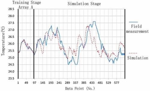
Figure 6. The simulation results using model trained by Array B.

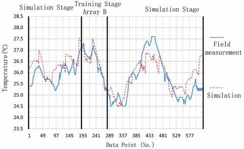
Figure 7. The simulation results using model trained by Array C.

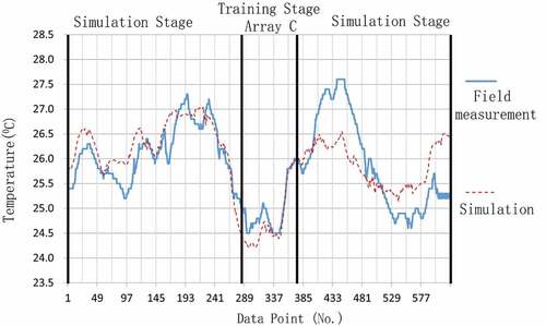
Figure 8. The simulation results using model trained by Array D.

(22) $MMean=\frac{1}{624}\sum _{k=1}^{624}{X}^{\prime }{{ }_1}^{{ }^{(0)}}(k)$(22)

(23) $SMean=\frac{1}{624}\sum _{k=1}^{624}S{{\overline{X^{\prime }}}^{(0)}}_1(k)\hspace{0.17em}$(23)

(24) $\begin{array}{rl}& MeasuredStandardDeviation=\sqrt{\frac{\sum _{\mathrm{k}=1}^{624}{(\mathrm{X}{{\prime }_1}^{(0)}(\mathrm{k})-\mathrm{M}\mathrm{M}\mathrm{e}\mathrm{a}\mathrm{n})}^2}{624}}\end{array}$(24)

(25) $SimulatedStandardDeviation=\sqrt{\frac{{\displaystyle \sum _{k=1}^{624}{(S{\overline{X^{\prime }}}^{(0)}{ }_1(k)-SMean)}^2}}{624}}$(25)

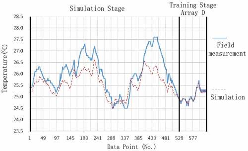
Table 3. The mean and the standard deviation between the measurement and simulation.

	Measured	Simulated by Array A	Simulated by Array B	Simulated by Array C	Simulated by Array D
Mean (°C)	25.86	25.85	26.06	25.91	25.19
Standard deviation (°C)	0.82	0.56	0.67	0.72	0.37

The measured indoor temperature provides the base for analysis of accuracy of simulation. The relative deviation between the simulated and the field measured indoor temperature is noted by RD. RD is calculated by Formula (26),

(26) $RD=\frac{abs(X^{\prime }{1}^{(0)}(k)-S{{\overline{X^{\prime }}}^{(0)}}_1(k))}{X{{\prime }_1}^{(0)}(k)}\times 100\mathrm{\%},k=1,2,\dots ,624$(26)

MRD is the arithmetic mean of relative deviation between the simulated and the field measured indoor temperature, calculated by Formula (27). MD is the mean deviation between the simulated and the field measured indoor temperature, calculated by Formula (28). SMSD is the standard mean square deviation between the simulated and the field measured indoor temperature, calculated by Formula (29). The lesser of deviation means the higher simulation accuracy. The calculated simulation accuracy of trained models is listed in Table 4.

(27) $MRD=\frac{1}{624}{\displaystyle \sum _{k=1}^{624}\frac{abs(X{\text{'}}_{\text{1}}{ }^{(0)}(k)-S{\overline{X^{\prime }}}^{(0)}{ }_1(k)}{X_{\text{1}}^{\text{'}}{ }^{(0)}(k)}}\times 100\%$(27)

(28) $MD=MRD\times \frac{1}{624}\sum _{k=1}^{624}{X}^{\prime }{{ }_1}^{(0)}(k)$(28)

(29) $SMSD=\sqrt{\frac{{\displaystyle \sum _{k=1}^{624}(X^{\text{'}}{{ }_{\text{1}}}^{(0)}(k)-S{\overline{X^{\prime }}}^{(0)}{ }_1{(k)}^2}}{624}}$(29)

Table 4. The accuracy of simulation using trained model.

	Array A	Array B	Array C	Array D
MRD (%)	1.76	1.73	1.64	1.43
Max of RD (%)	6.16	6.32	5.16	5.09
MD (°C)	0.46	0.45	0.42	0.37
RMSD (°C)	0.65	0.61	0.54	0.55

In term of Table 3, the maximum MRD is 1.76% of model trained by Array A, whereas the minimum MRD is 1.43% of model trained by Array D. The Maximum RD is 6.32% of model trained by Array B, whereas the minimum RD is 5.09% of model trained by Array D. The maximum MD is 0.46°C of model trained by Array A, whereas the minimum MD is 0.37°C of model trained by Array D. The maximum SMSD is 0.65°C of model trained by Array A, whereas the minimum SMSD is 0.54°C of model trained by Array C. It is clear that the selection of train data in this measurement provides consistent simulation value, meanwhile the selection of train data does not result in distinctive simulation accuracy. Therefore, the proposed model has been validated by the selection of train data.

The requirement for accuracy of measurement instrument of temperature is ±0.5°C in term of “Evaluation standard for indoor thermal environment in civil buildings” (GBT50785-2012) (MOHURD 2012) in China. Although an exact accuracy requirement for the indoor temperature simulation in civil building is not found by the current knowledge of authors, the requirement for accuracy of measurement instrument of temperature could provide a reference for the bench mark for simulation. Table 4 shows that the MD is lower than 0.5°C, and the SMSD is close to 0.5°C. Therefore, the accuracy of simulation of the proposed model is satisfactory for the assessment of indoor thermal environment in existing civil building.

6. Discussion

Two simulation models based on data mining are executed, respectively, to provide comparison for analysis of the performance of the proposed simulation model. The simulation model based on OGM(1,N) and the simulation model based on Elman neural network are executed, respectively. The proposed model in this paper is based on the combination of OGM(1,N) and Elman neural network. The four parent arrays of field measurement in the case building are inputted into model based on OGM(1,N) to train it, respectively. The four parent arrays are inputted into model based on Elman neural network to train it. The array of explanatory variables is inputted into the trained models to yield simulated indoor temperature. The comparison of simulation results using models trained by Array A is listed in Figure 9. The comparison of simulation results using models trained by Array B is listed in Figure 10. The comparison of simulation results using models trained by Array C is listed in Figure 11. The comparison of simulation results using models trained by Array D is listed in Figure 12.

Figure 9. The comparison of simulation results using models trained by Array A.

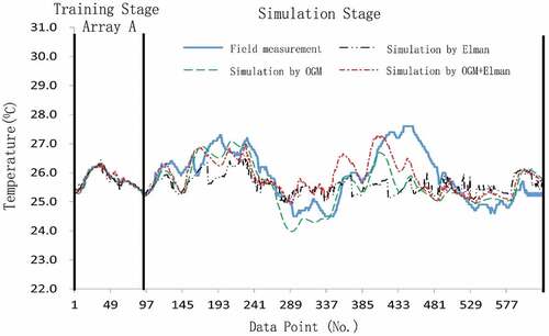
Figure 10. The comparison of simulation results using models trained by Array B.

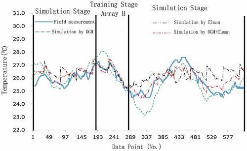
Figure 11. The comparison of simulation results using models trained by Array C.

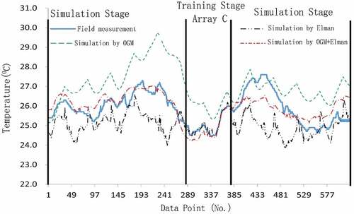
Figure 12. The comparison of simulation results using models trained by Array D.

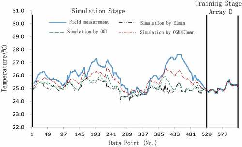
The patterns in Figures 9–12 indicate two features. Firstly, the simulation value of the model based on the combination of OGM(1,N) and Elman neural network has highest consistent with the field measured indoor temperature among the models. Secondly, the combination model has stronger robustness than the other two models. Evidence is that the selection of parent array has greater impacts on model of OGM(1,N) and model of Elman neural network than the combination model. Figure 9 shows that the model of Elman neural network trained by Array A has the biggest deflection from the measurement. Figure 11 shows that both of the model of Elman neural network and the model of OGM(1,N) trained by Array C have clear inconsistent with the field measurement. Though OGM(1,N) optimizes GM(1,N), minor fluctuation still exists in the structure of grey model. The structure of grey model causes the weakness of robustness of model of OGM(1,N). The small size of input data is the main reason for the insufficiency of model of Elman neuron network in this study. It is clear that the simulation performance of combination model is strengthened by the compensation from each other of grey system and neuron network in accuracy and robustness.

The comparison of simulation accuracy is listed in Table 5. The simulation accuracy of the model based on the combination of OGM(1,N) and Elman neural network is the highest among the models.

Table 5. Simulation accuracy of compared models.

		OGM (1, N)	Elman neural network	Combination of OGM and Elman neural network
Array A	MRD (%)	1.93	2.26	1.76
	Max of RD(%)	7.71	8.26	6.16
	MD(℃)	0.50	0.58	0.46
	SMSD(℃)	0.71	0.80	0.65
Array B	MRD%	2.14	2.79	1.73
	Max of RD(%)	7.32	8.35	6.32
	MD(℃)	0.55	0.72	0.45
	SMSD(℃)	0.71	0.90	0.61
Array C	MRD%	4.76	3.37	1.64
Array D	Max of RD(%)	12.21	11.36	5.16
	MD(℃)	1.23	0.87	0.42
	SMSD(℃)	1.42	1.15	0.54
	MRD%	2.89	3.06	1.43
	Max of RD(%)	9.03	10.15	5.09
	MD(℃)	0.37	0.79	0.37
	SMSD(℃)	0.99	1.06	0.55

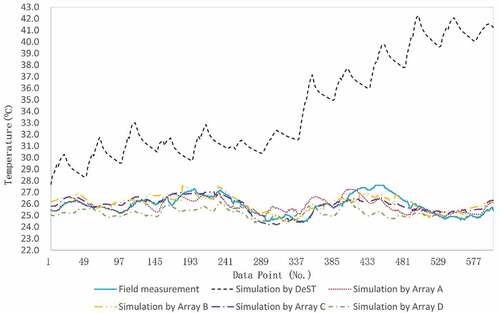
The simulation tool DeST is executed to provide further comparison, DeST is a kind of physics-based thermal simulation tool. The simulation indoor temperature of DeST and proposed simulation models in this paper are mapped in Figure 13. The indoor temperature of DeST has a great gap over the field measured value. A reason for the gap is that the outdoor climate embodied in DeST is a typical year data which has a deviation from the field measured value of outdoor environment. Another reason for the gap is that the operation of the building is different from the pattern of design embodied in DeST. Compared with the simulation indoor temperature of DeST, the model of combination of OGM(1,N) and Elman neural network is highly consistent with the field measured indoor temperature. It is evident that the proposed model suits for the thermal environment simulation in existing buildings, whereas DeST suit for the design stage for building thermal environment.

Figure 13. The indoor temperature of simulation by OGM+Elman model, simulation by DeST and field measurement.

7. Summary and outlook

Simulation of the indoor temperature provides important references for thermal environment not only for design of building but also for assessment of existing buildings. The current thermal environment simulation software tools suit for building design stage, however do not suit for existing buildings. Field measurement is a convincing assessment method of indoor thermal environment in existing buildings, however measurement of long period is high cost and cause more disturbances to occupants. Small size field measured data is commonly available in building thermal assessment practices in term of “Evaluation standard for indoor thermal environment in civil buildings” (GBT50785-2012). Therefore, there is a need for prediction of indoor thermal environment under short-term field measured data in both practical and academic research. This study aims to provide more reference for indoor thermal environment assessment and design. This research is summarized as follows:

1. A model is proposed to simulate indoor temperature, which is trained by small size field measured data in existing building. The proposed model is on the combination of OGM(1,N) and Elman neural network. OGM(1,N) has convincing modelling ability in mining of the small size data, however, it is lack of self-adaptation and parallel computing ability. Elman neural network has strong self-adaptability and fault tolerance in prediction, however the high performance of Elman neural depends on the big size of training data. Therefore, the combination of OGM(1,N) and the Elman neural network compensate for each other in stable structure and accuracy with small size training data.

2. A unit is designed and installed in a case building in Hangzhou of China to measure and record thermal parameters, the field measurement is carried out in for a year at interval of half hour, covering indoor temperature, outdoor temperature, outdoor relative humidity, outdoor wind velocity and the recording time. Twelve days field measured data in the second season in natural ventilated building are selected as the database, four selected 2 days of field measured data are used to train the proposed model respectively, the remaining data is used to validate the proposed model. The process of training and validation of the proposed model is implemented by programming in Matlab. The validation of the proposed model is demonstrated by the analysis of consistency and accuracy between the simulation indoor temperature and the field measured data.

3. Two simulation models driven by data mining, the simulation model based on OGM(1,N), the simulation model based on Elman neural network, are executed respectively to provide comparison for the proposed simulation model. The simulation indoor temperature of the model based on the combination of OGM(1,N) and Elman neural network has highest consistent with the field measured indoor temperature. The simulation accuracy of the model based on the combination of OGM(1,N) and Elman neural network is the highest among these three models. The combination model has stronger robustness than other two models. The simulation tool DeST is executed to provide further comparison, it is evidential that the proposed model suits for the thermal environment simulation for existing buildings, whereas DeST suits for the design stage for buildings.

It is the wish of authors that the following issues will be investigated to strengthen this study in the future.

1. It is observed a relatively big gap between the simulation indoor temperature and the field measurement on the range of peak value in simulation stage in Figures 5–8. It will be investigated how the peak value of explanatory variables in the extended period influence on the model.

2. This study was carried out in the second season. How the model work in other seasons, special in the third season, it is worth being further validated in the future. In summer and winter, the cooling system and heating system becomes the main explanatory variable, how this model is revised to provide reference for thermal environment assessment, it will be investigated in the futher.

Disclosure statement

No potential conflict of interest was reported by the author(s).

Additional information

Funding

This research is financially supported by Zhejiang Provincial Natural Science Foundation of China under Grant No. LY18E080035, National Social Science Fund of China under Grant No. 20BZX132.

Notes on contributors

Yulan Yang

Yulan Yang,Phd,Associate Professor, she is interested in research of building indoor environment,building energy efficiency and historic building conservation.

Huixin Tai

Huixin Tai,Phd,Associate Professor, he is interested in research of architectural acoustics and historic building conservation.

Lingzhi Liu

Lingzhi Liu,Phd, Professor, she is interested in research of built environment and historic building conservation.

Beier Yu

Beier Yu,he is a postgraduate student.

Wenlong Song

Wenlong Song,he is a postgraduate student.

References

- Afroz, Z., G. M. Shafiullah, and G. Higgins. 2017. “Prediction of Indoor Temperature in an Institutional Building.” Energy Procedia 142: 1860–1866. doi:10.1016/j.egypro.2017.12.576.
- Amirul, I. K., D. C. Nicolas, J. N. Catherine, and S. Jonathan. 2017. “Real-time Flow Simulation of Indoor Environments Using Lattice Boltzmann Method.” Building Simulation 2015 (8): 405–414.
- Andarini, R. 2014. “The Role of Building Thermal Simulation for Energy Efficient Building Design.” Energy Procedia 47: 217–227. doi:10.1016/j.egypro.2014.01.217.
- Antoni, W., and L. C. Macie. 2016. “Elman Neural Network for Modelling and Predictive Control of Delayed Dynamic Systems.” Archives of Control Sciences 26 (1): 117–142. doi:10.1515/acsc-2016-0007.
- Bezuglov, A., and G. Comert. 2016. “Short-term Freeway Traffic Parameter Prediction: Application of Grey System Theory Models.” Expert Systems With Applications 62: 284–292. doi:10.1016/j.eswa.2016.06.032.
- Chen, X., and M. Liu. 2017. “Simulation and On-site Measurement of Heating Performance in Air-conditioned University Dormitories, a Case Study in Chongqing.” Procedia Engineering 205: 2569–2576. doi:10.1016/j.proeng.2017.10.235.
- Cornick, S. M., and M. K. Kumaran. 2014. “A Comparison of Empirical Indoor Relative Humidity Models with Measured Data.” Journal of Building Physics 31 (3): 25.
- Deng, J. L. 1982. “Control Problems of Grey Systems.” Systems & Control Letters 1 (5): 288–294. doi:10.1016/S0167-6911(82)80025-X.
- Deng, J. L. 1986. Grey Prediction. Wuchang: Huazhong University of Science & Technology Press. in Chinese
- DeST. 2022. Accessed 19 April 2022. https://www.dest.net.cn/zy
- Elman, J. L. 1990. “Finding Structure in Time.” Cognitive Science 14: 179–211. doi:10.1207/910s15516709cog1402_1.
- Giacomo, C., L. S. Grazia, and M. C. Cammarata. 2017. “Thermal Transients Simulations of a Building by a Dynamic Model Based on thermal-electrical Analogy: Evaluation and Implementation Issue.” Applied Energy 199 (1): 323–334. doi:10.1016/j.apenergy.2017.05.052.
- Guo, Y., X. Wu, J. Chen, and X. Zhang. 2014. “Measured Data Verification of Energy Consumption in a Green Building for Building Energy Simulation Software eQUEST Model.” Building Energy Efficiency 42: 88–291.
- Jiao, L., S. Yang, F. Liu, S. Wang, and Z. Feng. 2016. “Seventy Years Review of Neural Networks: Retrospect and Prospect.” CHINESE JOURNAL OF COMPUTERS 39 (8): 1697–1716.
- Lin, Y., and S. Liu. 2000. “A Systemic Analysis with Data (II).” International Journal of General Systems 29 (6): 989–999. doi:10.1080/03081070008960982.
- Martínez-Ibernón, A., C. Aparicio-Fernández, R. Royo-Pastor, and J. L. Vivancos. 2016. “Temperature and Humidity Transient Simulation and Validation in a Measured House without a HVAC System.” Energy and Buildings 131: 54–62. doi:10.1016/j.enbuild.2016.08.079.
- MOHURD. 2012. “Evaluation Standard for Indoor Thermal Environment in Civil Buildings (GBT50785-2012).” Ministry of Housing and Urban-Rural Development of the People’s Republic of China (MOHURD). (in Chinese)
- Sahar, A., M. N. SeyedMorteza, M. Hosein, G. Rohit, Z. Rong, and K. P. Shwar. 2021. “A gray-box Model for real-time Transient Temperature Predictions in Data Centers.” Applied Thermal Engineering 185: 116–319.
- Sözer, H., and S. S. Aldin. 2019. “Predicting the Indoor Thermal Data for Heating Season Based on short-term Measurements to Calibrate the Simulation set-points.” Energy & Buildings 202: 1–11. doi:10.1016/j.enbuild.2019.109422.
- Thananchai, L. 2008. “Grey Prediction on Indoor Comfort Temperature for HVAC Systems.” Expert Systems with Applications 34 (4): 2284–2289. doi:10.1016/j.eswa.2007.03.003.
- Wang, W., L. Cai, and S. Wang. 2015. “Modelling and Analysis of Meteorological Factors’ Impact on Building Indoor Temperature.” Computer Simulation 32 (6): 338–343,372.
- Wang, S., P. Wang, and Y. Zhang. 2020. “A Prediction Method for Urban Heat Supply Based on Grey System Theory.” Sustainable Cities and Society 52: 101–819. doi:10.1016/j.scs.2019.101819.
- Wu, Q., S. Wang, and Y. Yang. 2012. “Research the Deformation Prediction System of Foundation Pit Based on Grey Theory.” Applied Mechanics & Materials 170-173 (4): 170–173. doi:10.4028/scientific.net/AMM.170-173.174.
- Yang, Y., S. Liu, and G. Ying. 2015. “Building Energy Use Behavior Measuring and Recording Device for Distributed air-conditioned Space.” China Patent CN201510577821, November 11. (in Chinese)
- Zeng, B., C. Luo, S. Liu, Y. Bai, and C. Li. 2016. “Development of an Optimization Method for the GM(1,N) Model.” Engineering Applications of Artificial Intelligence 55 (2016): 353–362. doi:10.1016/j.engappai.2016.08.007.
- Zeng, B., X. Yin, and W. Meng. 2018. Practical Modelling Method of Grey Prediction and Programming in Matlab. Beijing: China science publishing & Media . (in Chinese)