Web-based approach for systematic analysis and interactive visualization of the industry foundation classes data: a case study in duct design

ABSTRACT

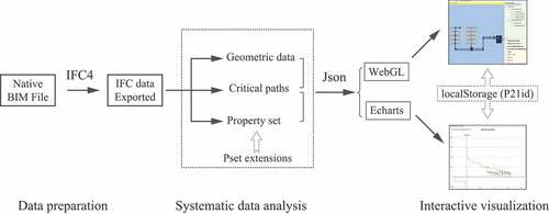
Existing model checkers of building information modeling (BIM) can open industry foundation classes (IFC) files and perform clash detection between mechanical, electrical, and plumbing (MEP) and architectural as well as structural models. However, there are few applications of IFC data in MEP engineering, specifically in interactive visualization between calculation results and BIM models. This study focuses on the systematic analysis of a BIM model and interactive visualization of IFC data for MEP engineering. First, the systematic analysis method for a ventilation system is proposed using the critical path class. Second, referring to the IFC relationship of connections between duct elements, elements in the same system are sorted into different levels of critical paths. Furthermore, ifcPressureViewer is developed based on the interactive visualization methodology by connecting Three.js, a JavaScript 3D library, with Echarts, a JavaScript visualization library, which is applicable for desktop computers and mobile tablets. This is followed by a case study that demonstrates the application of the interactive visualization process. Finally, the conclusions of this study are summarized, and directions for future research are discussed.

GRAPHICAL ABSTRACT

KEYWORDS:

• IFC-Property sets
• critical path
• node
• pressure loss
• balancing rate

1. Introduction

Testing, adjusting, and balancing (TAB) is crucial for checking and adjusting all environmental systems in a building to meet the design objectives. For a ventilation system, the American Society of Heating, Refrigerating, and Air-Conditioning Engineers (ASHRAE) suggests balancing the sub-main air ducts first, then the branch ducts, and finally the flow rates of the air terminal devices (ASHRAE 2019). Balancing devices such as dampers and blast gates are often recommended to be installed. However, it is not economical to rely entirely on dampers to balance the ductwork because of flow-generated noise from the dampers. Additionally, systems could be balanced by changing the resistance to duct sections, such as changing duct size, selecting different fittings, and increasing airflow.

Total pressure grade line (ASHRAE 2017), which illustrates the variation in pressure loss along the duct path, is often used in duct design. The pressure losses caused by friction and dynamic losses between sections are often used, whereas detailed pressure losses for straight ducts and fittings are not available. How to change the resistance of a duct section? There are several options to achieve this, such as adjusting the damper, selecting a different fitting, or changing the duct size. However, it may be difficult to choose the optimal approach for this purpose. Therefore, visualization of the detailed pressure losses of ducts and fittings is necessary.

The specification of industry foundation classes (IFC) developed by buildingSMART defines a conceptual data schema and an exchange file format for building information modeling (BIM) data (ISO 2013). Focusing on interactive visualization between the 3D model and the performance data for duct design, ifcPressureViewer, a web application, is developed using the IFC data and the Property sets (Psets) exported by the BIM software.

This paper first introduces a background on the current applications of IFC data in the mechanical, electrical, and plumbing (MEP) engineering, as well as the interactive visualization tools. Thereafter, a systematic analysis method for ventilation system is conducted using the critical path class proposed. Referring to the connectivity relationship between distribute elements in a supply system defined in IFC4 specification, elements in the same system are sorted into different levels of critical paths. Furthermore, ifcPressureViewer, a web application, is developed based on the interactive visualization methodology by connecting Three.js, a JavaScript 3D library, with Echarts, a JavaScript visualization library. Three.js is used to visualize the geometric attributes of the IFC data, while Echarts is for Psets of pressure loss and duct length. This is followed by a case study that demonstrates the application of the interactive visualization process, which is available for desktops, laptops, tablets, and even smartphones. Finally, the conclusions of this study are summarized, and directions for future research are discussed.

2. Literature review

2.1. Application of IFC data

IFC specification is a neutral, open-file format that provides a platform for data exchange throughout the life cycle of building projects. Park et al. (2018) described an information modeling method for steel box girder bridges based on IFC and estimated the carbon emission from the superstructure of a steel bridge model using the quantity take-off and proposed user-defined Psets of each component. The detailed quantities and carbon emissions are listed in text boxes. G. Benndorf et al. (Benndorf et al. 2017) described the application of IFC in building automation and control systems (BACS) and extended IFC files exported from a BIM tool for heating, ventilation, and air-conditioning (HVAC) control using the open-source library IfcOpenShell. Referring to the relationship class IfcRelNests, the sensor, actuator, and controller are connected by ports defined by the IfcDistributionPort class in the temperature-controlled heating circuit. Psets, such as heating curve and time schedule are added to the circuit. This application is one of the examples of using IFC in MEP engineering, but it lacks the description of the whole heating circuit and the control system.

Using an IFC mapping file, the BIM software can export or import the IFC files of the building models. BIM model checkers, such as Solibri Anywhere (Solibri 2020), BIMServer (CYPE 2021), BIMVision (Datacomp 2021), and Navisworks Manage (Autodesk 2020a), can open an IFC file, visualize the 3D model, and display the IFC attributes of each element. Some of them can even highlight all the elements in the same system. But there is no clarity in the detail performance data about the MEP system, such as the length of a duct path from the air handling unit (AHU) to a terminal, the air balance at the diverging or junction fitting, and the total pressure loss in the critical path. Compared with the individual elements in an architectural model, the performance data of the duct path and the entire system should be emphasized in a MEP model. Therefore, systematic analysis is considered a requisite for MEP engineering.

2.2. Visualization of the IFC data based on WebGL

WebGL has often been used to render 3D graphics of building elements in BIM applications. A WebGL-based IFC visualization method was proposed to convert the IFC text into an object file (with the format of OBJ), including the IFC attributes, create 3D visualizations using JavaScript programming, and visualize the IFC file in a web browser (Xu, Zhang, and Xu 2016). Based on the conversion of IFC into 3D tiles using caesium, Xu et al. proposed a data integration approach to visualize the BIM in a web browser via Node.js, which was available for IFC files with a large size (Xu et al. 2020). Lu et al. proposed a method for loading large IFC files based on spatial semantic partitioning (SSP) using WebGL, and the BIM models were partitioned by story, which reduced the memory consumption for network visualization (Lu et al. 2019). Tanaka et al. proposed a WebGL model to support the detection of bridge maintenance information using Python to build a server and the IFC Engine DLL to convert the IFC model into a triangular mesh and realize visualization on the client side via Three.js (Tanaka et al. 2016). Wang et al. transformed the OBJ format geometric data exported by Revit into JSON data and used Three.js to visualize an ancient building in the browser (Wang and He 2020). These applications are proposed for desktop computers.

WebBIM, a cross-platform online visualization system based on IFC and WebGL, converts the raw IFC geometry data into triangles, reduces the size of BIM geometry data, and renders the decompressed triangular BIM data directly in a web browser (Zhou et al. 2019). This application realized the visualization of IFC data on mobile tablets.

Although IfcOpenShell has often been used many studies (Moretti et al. 2020; Wang and Issa 2020), the IFC data in this study are parsed with referring to Python-ifc developed by Marijn van Aerle (van Aerle 2013). The geometric attributes of elements are calculated according to coordinate transformation matrix from the geometric shape and local placement attributes of an IfcElement (Xu and Aadachi 2020) and converted into JSON format. The visualization of duct elements is realized using Three.js, which is also available for mobile tablets.

2.3. Application of interactive web application

Some BIM tools provide the highlight function for viewing the elements. For example, an element can be highlighted in a 3D/2D model by clicking in the element’s cell in the schedule/quantities or material take-off view (Autodesk 2020b). It helps in connecting the element from the schedule view to building model, but this kind of communication is only a one-way process.

HTML web storage provides localStorage for objects to store data that can be used for data interconnection. A web server security evaluation method is proposed using Echarts and the HTML5 localStorage between the pages to interconnect the data (Wu, Gao, and Liu 2018). Lee et al. designed and implemented an interactive collaboration platform, V3DM+, for facility management, which links the information data with the 3D model through a specific ID. This system can be applied to the maintenance and operation phase of BIM (Lee et al. 2016). Vanlande et al. Use IFC files for data sharing in facility management, which provides interactive links between 3D models and information data (Vanlande, Nicolle, and Cruz 2008).

Echarts, an open-source JavaScript visualization library developed by Baidu, supports the rapid construction of interactive visualization. It provides various chart types and visual channels, such as color, lightness, size, and glyph, which can be encoded for different levels of data (Li et al. 2018). A multi-scale visualization method for bus travel speed was proposed using Echarts and WebGL to analyze traffic congestion in urban public transport networks, which illustrated the average travel speed on arterial roads by a heat map (Yong et al. 2016). Lu et al. proposed a visualization interaction method based on the Baidu map API, Echarts, and jQuery to develop a WebGL-based 3D visualization platform for rapid earthquake reporting. They used Echarts and memory optimization techniques to optimize the display for mobile terminal platforms (Jiang, Wang, and Zhu 2016). These applications show that Echarts is available for mobile tablets.

In this study, we use Python Flask to build a web server and sent the pressure data of the duct systems to the client in the form of JavaScript object notation (JSON). The BIM model is visualized using WebGL, and the pressure distribution is visualized using the 2D line segments of Echarts. The interactive visualization between the BIM model and the 2D line segments is realized using the HTML5-based localStorage.

2.4. The novelty and focus of this study

This study focuses on the interactive visualization of IFC data and systematic analysis of BIM model for MEP engineering. The performance data of pressure distribution of the ductwork are integrated with the BIM model. Compared with existing BIM tools and model checkers, the proposed approach has the following highlights:

1. Systematic analysis for a ventilation system using IFC data: 

The systematic analysis for a ventilation system is carried out using the critical path class proposed. The duct elements in the same system are sorted into different levels of critical paths by searching the IFC relationship between the elements.

(2) Interactive visualization:

ifcPressureViewer, a lightweight BIM tool, is developed to visualize the pressure distribution and BIM model using Flask, WebGL and Echarts, which can be used on desktop computers and mobile tablets. P21id of an IfcElement, a uniform resource identifier (URI) in an IFC file (a text format defined by ISO 10303–21) (ISO 2017), is stored in the HTML5-based localStorage for interaction between the BIM model and pressure distribution.

Ventilation system is one of the typical distribution systems, and the systematic analysis method proposed will also be available for other MEP systems. Furthermore, the lightweight ifcPressureViewer is applicable for both desktops and mobile tablets, which will be helpful for using IFC data in duct design and construction.

3. Systematic analysis method for a distribution system

3.1. Schematic description of a distribution system

A distribution system shown in Figure 1 can be applied for air, water, and power supply. Systematic analysis of the grouped objects in a system concerns the domain-specific knowledge. For a ventilation system, air is supplied by the AHU/fan (abbreviated to AHU), which is the starting point of a duct route. To realize the supply air volume at each terminal, the endpoint of a route, is the goal of duct design.

Figure 1. Schematic layout of a simple distribution system.

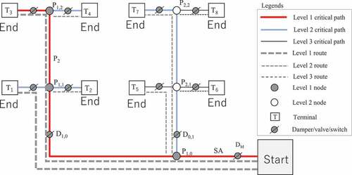
The equal friction method is often used in duct design for sizing lower-pressure supply air, return air, and exhaust air duct systems. To realize the air volume at the most remote terminal, the total pressure of the system is calculated by adding up the pressure loss of each element in the critical path (the path with the highest overall pressure loss). The major disadvantage of this method is that there is no provision for equalizing pressure drops in duct branches. A manual balance of short runs to achieve the same pressure drop as a long branch run is required (McDowall 2010; Behls 2021; Bhatia 2001).

Therefore, we use different levels of critical paths and nodes to describe a duct system in this study. The route from AHU to T₃, the most remote terminal, is called the level 1 critical path. Air balance at diverging fittings such as P_1,0, P_1,1 and P_1,2, is essential for duct design, which are called level 1 nodes. Duct routes downstream from these nodes are called level 2 duct routes. There will be a critical path in each branch flow direction of a level 1 node. Similar to the level 1 critical path, the level 2 critical path is decided by comparing the total length of each straight duct in each level 2 route. The diverging points in a level 2 path such as P_2,1 and P_2,2, are called level 2 nodes. A similar analysis can be applied to the next level of critical path.

3.2. Proposition of critical path class

Critical path class is proposed for ductwork analysis, and its attributes are detailed as follows (Table 1).

Table 1. Definition of the critical path class.

No.	Attribute name	Description
1	Level	Level number of the critical path.
2	StartPoint	Starting point of the critical path.
3	EndPoint	Endpoint of the critical path.
4	Elements	A list of elements in the path.
5	Nodes	A list of diverging/merging points in the path
6	Length	The total length of each straight duct/pipe in the path.

1. The “Level” attribute is the level number of a critical path.

2. The “StartPoint” attribute is the starting point of a path. For a ventilation system, AHU/fan will be the starting point of the level 1 critical path, and the diverging/merging point will be the starting point of the next level critical path.

3. The “EndPoint” attribute is a terminal, the end point of a critical path.

4. The “Elements” attribute consists of a list of elements in the path, including the AHU, duct fittings and terminal.

5. The “Nodes” attribute consists of a list of diverging/merging points in the path. Each node is the starting point for the next level path. If there is no diverging/merging point, the value will be “NULL”.

6. The “Length” attribute is the total length of each straight duct/pipe in the path.

According to the critical path class definition, the above simple system can be described as shown in Figure 2. There is one level 1 path starting from AHU and ending at T₃, four level 2 paths (such as the path starting from P_1,0 to T₇ and that starting from P_1,2 to T₄) and three level 3 paths (such as the path starting from P_2,1 to T₅ and that starting from P_2,2 to T₈).

Figure 2. Schematic description of a system by the critical path class.

3.3. Connection between elements upstream and downstream

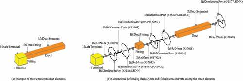
Figure 3 gives an example to illustrate the connectivity relationship between the upstream and downstream elements of the duct in the supply system. Figure 3(a) shows the three connected duct elements: downstream air flow terminal with the name of Terminal, the connected duct fitting (Fitting) and the upstream duct (Duct). While the connections defined by IfcRelNests and IfcRelConnectsPorts among these three elements are shown in Figure 3(b). The sorting method from Terminal to upstream Duct can be explained as follows:

1. Referring to INV:NestedBy¹ attribute of Terminal, the connected IfcRelNests (#37809) is obtained.

2. Among the RelatedObjects attribute of IfcRelNests (#37809), the connected upstream IfcDistributionPort (#35862) can be obtained because its flow direction is “SINK”.

3. According to the INV: ConnectedTo attribute (inverse attribute with the name of ConnectedTo) of IfcDistributionPort (#35862), IfcRelConnectsPorts (#35869) can be obtained.

4. According to the RelatedPort attribute of IfcRelConnectsPorts (#35869), the connected upstream IfcDistributionPort (#35867) can be obtained because its flow direction is “SOURCE”.

5. The upstream Fitting can be obtained from the INV: Nests attribute (inverse attribute with the name of Nests) of IfcDistributionPort (#35867), IfcRelNests (#37093).

6. Similarly, referring to the above steps (1) to (5), the upstream Duct can also be obtained.

Figure 3. Example of connectivity relationships among duct elements.

Therefore, all elements in the same route can be sorted by a recursive function in programming from downstream to upstream.

3.4. Critical path and attribute obtaining

According to the definition of IfcRelAssignsToGroup shown in Figure 4, the name and type of a system are defined in the RelatingGroup attribute, and the related objects, including the ports are grouped in the RelatedObjects attribute. The duct elements in the same system can be sorted into different levels of critical paths by searching the IFC relationship between the elements. The details are shown as follows:

Figure 4. Definition of IfcRelAssignsToGroup.

Step 1: Searching the duct elements in a route.

As shown in Figure 5, search each terminal (the endpoint of a route) among the related duct elements in the IfcRelAssignsToGroup. The upstream element of the terminal can be obtained with referring to the connectivity relationships among duct elements described in Section 3.3. It comes to the endpoint of a route when the upstream element is AHU (the starting point of a ventilation system) and searching the next upstream element when it is not. Therefore, all the elements in the same route can be obtained.

Figure 5. Flow chart for searching the routes.

Continue to search the next route until all the routes from each terminal to the AHU can be obtained.

Step 2: Comparing the length of each route to obtain the critical path.

Compare the length of each route in the routes obtained in Step 1 (Figure 5), and the longest one will be the critical path. For each element in this path, add it into the “Elements” attribute of this path (Figure 6). Then examine the connected ports of the element. When the number of connected ports is larger than two, the element will be a node and add it into the “Nodes” attribute. For example, a fitting, such as Tee, has three ports. Thus, to obtain the critical path, as well as the attributes shown in Table 1.

Figure 6. Flow chart for obtaining the critical path.

Step 3: Searching the next level critical path(s) and elements, including the geometric attributes.

For each terminal not grouped in the level 1 critical path acquired, continue the processes illustrated in Steps 1 and 2 to obtain the elements and nodes in the level 2 critical path. For a level 2 route, it ends at one of the nodes in the uplevel. If the node has two or more branch flow directions, the next level critical path will be obtained by comparing the length of each route in each branch direction.

The systematic analysis is carried out by a recursive function in Python programming until all the elements in all duct paths are found. Therefore, all the terminals and elements are grouped by critical paths at different levels.

4. Methodology to interact the visualization of the 3D model with pressure distribution line

Pressure distribution is an important performance factor in MEP engineering, especially the balancing rate at the diverging and converging fittings. We used the pressure distribution line for system performance check. The dynamic losses at the fittings, dampers, or equipment are visualized, as well as the friction losses of the straight ducts or pipes.

According to the IFC data exported from the native BIM file, Figure 7 illustrates a three-step methodology that enables the interactive visualization of a 3D model and pressure distribution line. The details are as follows:

Figure 7. Flow chart for interactive visualization.

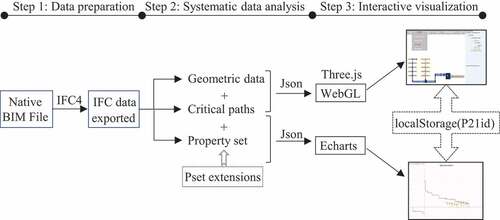
Step 1: Data preparation.

IFC data of a native BIM file are exported with the version of IFC4, which consist of MEP elements, attributions, and the grouping relationship. The geometric attributions, such as shape representations and placements, are exported, as well as the Psets.

In this study, the mechanical-flow and dimension Psets of duct elements in a ventilation system, such as flow rate, pressure loss and length, are used, as well as the grouping relationship defined by IfcRelAssignsToGroup and the connections defined by IfcRelNests and IfcRelConnectsPorts.

Step 2: Systematic data analysis and Psets.

Step 2–1: Geometric attributes converted into JSON format.

According to the systematic analysis method proposed, duct systems, including duct elements, are grouped by critical paths. The geometric attributes of elements such as placement and shape representation are calculated and converted into JSON format. Geometric representation, such as swept solid (SweptSolid) and boundary representation (Brep) models is handled in this study.

Step 2–2: Psets converted into JSON format.

Psets of duct elements with flow rate, pressure loss and duct length are obtained. The pressure losses at the nodes differ in the flow directions, but only one pressure value is exported by the BIM tool used in this study. Therefore, Pset extensions for nodes are considered. The custom input method for fitting pressure-loss Pset is proposed, directly interacting with the 3D model.

Step 3: Interactive visualization.

Step 3–1: Visualization of the 3D model.

According to the geometric attributes of duct elements converted into JSON format, the geometric data are processed into triangular mesh structures by calling Three.js. Thus, to realize the visualization of the 3D model.

Step 3–2: Visualization of pressure losses of duct elements and critical paths.

According to the pressure loss Psets of duct elements converted into JSON format, the pressure data are processed into a line by Echarts.js. Thus, to realize the visualization pressure loss of each element. The vertical lines represent the dynamic losses at the fittings, dampers, or equipment, whereas the slanting lines (nearly horizontal) represent the friction losses of the straight ducts. The pressure distribution along the critical paths and pressure balance at the nodes are also visualized by Echarts.

Step 3–3: Interaction between the 3D model and pressure lines.

The interaction between the 3D model and the pressure loss data is realized using the P21id of each IfcEnitity stored in the JavaScript localStorage object. Query the P21id every 1 ms, thus, to interact the element in the 3D model with the pressure line.

ifcPressureViewer is developed to visualize the pressure loss distribution using the IFC data, which responds to UI and tool events in the browser with queries. We used the Flask server to create interactive web applications that connected front-end UI events using python code.

5. Case study

Ventilation system is one of the distribution systems in MEP engineering. To ensure the desired flow rate of a ventilation and each terminal, especially the most remote terminal, is the goal of duct design. Each air duct system should be tested, adjusted, and balanced (TAB). The visualization of balancing rate at the diverging fitting is important for TAB personnel and others during the commission of duct systems. Therefore, a ventilation system is used for case study.

5.1. Ventilation system for case study and the interface of ifcPressureViewer

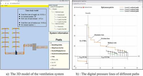
The ventilation system was created using Revit in the design phase. There are two duct systems here: one is “Mechanical Supply” system, and the other is “Mechanical Outdoor” system. The supply system comprises of an AHU, a silencer, a volume damper, and 20 air terminals each with the flow rate of 167 L/s. The outdoor duct system has only one terminal. The total flow rate of the ventilation system is 3333 L/s. The IFC data of this BIM model were exported with the following options provided by Revit: the version of IFC4 Design Transfer View, Revit Psets, IFC common Psets and base quantities. Figure 8 illustrates the interface of the developed ifcPressureViewer. The 3D model of the ventilation system is shown in Figure 8(a)), as well as the system information and Psets of selected duct element. While the digital pressure lines of different paths of the system are shown in Figure 8(b)). The vertical lines represent the dynamic losses at the fittings, dampers, or equipment, whereas the slanting lines (nearly horizontal) represent the friction losses of the straight ducts. The total pressure loss of the entire system was approximately 378 Pa. The total length of straight ducts in level 1 critical path for SA system is 32.5 m, while it is 8.3 m for OA system.

Figure 8. Ventilation system for case study and the interface of ifcPressureViewer.

5.2. Ductwork analysis and visualization of pressure loss

5.2.1. The custom input for fitting pressure-loss Pset

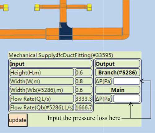
Since there is only one pressure loss value for tee or cross exported by the BIM tool used in this study. The custom method for adding fitting pressure-loss Pset is proposed. As shown in Figure 9, the custom pressure losses can be added by right clicking the mouse on the selected fitting. Referring to the dimensions and flow rates obtained from the IFC data, it will be convenient to add the pressure values.

Figure 9. Example for adding the custom pressure loss.

5.2.2. Duct systems grouped by critical paths and visualization of pressure loss

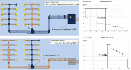
When the individual critical path is selected, it will be highlighted in the 3D model. The pressure loss on the path will also be available (Figure 10). The pressure loss on level 1 critical path is 307 Pa, and 62.1 Pa on the level 2 path selected.

Figure 10. Pressure losses for selected critical paths.

5.3. Interaction visualization between the BIM model and the pressure loss

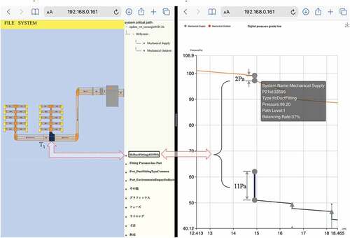
The line segment in the pressure chart is highlighted when one element in the 3D model is selected. The detailed pressure losses can be confirmed by enlarging the pressure line. Figure 11 illustrates the interaction of the 3D model with the pressure loss grade line on iPad. There were two pressure losses at T₁. One was 2 Pa in the main flow direction, and the other was 11 Pa in the branch direction. The total pressure at T₁ is 99.2 Pa in level 1 critical path, while the pressure is only 62.1 Pa in the level 2 critical path. Therefore, the balancing rate at T₁ (the node of level 1) is 37%, which is larger than the tolerances of ±10% suggested by ASHRAE. Because the pressure loss in the branch direction is lower, a damper is required in the branch duct. Conversely, the interaction can also be initiated from the pressure chart.

Figure 11. Interactive visualization between 3D model view and pressure chart.

5.4. Discussions about the proposed ifcPressureViewer

Three.js has been often used in visualization of BIM models. But the design results, especially the system performance data, have not been visualized. In this paper, we combined Echarts, a JavaScript visualization library with Three.js to realize the interactive visualization for BIM models.

Compared with the existing BIM model checkers, such as BIMvision, the proposed ifcPressureViewer provides a second window to realize the interactive visualization between the BIM model and the system performance data. Not only the text information of Psets of duct elements, but also the balancing rates at the different levels of critical paths can be visualized. Because the details of pressure losses at the diverging fittings can be distinguished in different flow direction, the designer and engineer can not only know the balancing rates, but also find the unbalanced fittings and improvement in balancing the pressure quickly. Furthermore, it will help the TAB personnel and others during the commission of duct systems.

While the BIM software, such as Revit and MagiCAD, can size the ducts, conduct system inspection, and even realize the interactive visualization between the calculation report and Revit model (MagiCAD Group 2021). But Revit can only be used on Windows desktop computers. The proposed ifcPressureViewer is lightweighted and can also be applicable on mobile tablets. Although the interactive visualization was realized between the 3D model and the pressure losses of selected critical paths, the methodology of interactive visualization proposed can be applied to other system performance data.

6. Conclusions

In this study, we proposed a systematic analysis method for a distribution system using the critical path class, and the system is described by different levels of critical paths and nodes. Referring to the connectivity relationship between distribute elements in a supply system defined in the IFC4 specification, the terminals, duct elements in the same system are sorted into different levels of critical paths. We then proposed the interactive visualization methodology by connecting Three.js with Echarts via HTML localStorage in a web browser. ifcPressureViewer, a web-based approach, was developed to visualize the pressure-loss distribution and BIM model.

Three.js was used to visualize the geometric attributes of the IFC data, while Echarts was for Psets of pressure loss and duct length. The custom input method for fitting pressure-loss Pset was also proposed, directly interacting with the 3D model.

Furthermore, ifcPressureViewer, was developed to visualize the pressure-loss distribution and the BIM model in a web browser. A case study utilized ifcPressureViewer in a ventilation system using the IFC data exported by a BIM tool. The results demonstrated that the pressure losses of the duct elements and the pressure balancing rate at the nodes were dynamically connected with the BIM model. It is also applicable for desktop computers and mobile tablets.

The proposed systematic analysis method for a distribution system can be used for air, water, and power supply. Most of the BIM software can export the geometric data of building elements and MEP elements, if the following IFC entities can be included in the exported IFC data, the proposed methodology for interactive visualization will be applicable to other MEP systems.

1. IfcRelAssignsToGroup: the system information of the MEP system, as well as the related elements.

2. IfcPort, IfcRelConnectsPorts, IfcRelNests: the connectivity relationship of elements. The flow direction value should be prescribed, and flow out port, the value should be SOURCE, and SINK for flow in port.

As to the geometric representation for an IfcProduct, only the Sweptsolid and Brep models are available in this study. Other models, such as constructive solid geometry (CSG) and clipping models, will be considered in the future.

Disclosure statement

No potential conflict of interest was reported by the author(s).

Data availability statement

The data that support the findings of this study are available on request from the corresponding author, [L.X.]

Additional information

Funding

This work was supported by JSPS KAKENHI Grant Number 21K04375

Notes on contributors

Hongxia Deng

Dr. Hongxia Deng is an Associate Professor in the Department of Computer Science, Taiyuan University of Technology. She received her Bachelor's, Master's and PhD degrees in engineering from Taiyuan University of Technology in 1998, 2006 and 2013, respectively.

Ying Liu

Mr. Ying Liu recently graduated from the graduate school of Taiyuan University of Technology. He received his B.E degree from Hebei Normal University, Shijiazhuang in 2019, and M.Eng degree from Taiyuan University of Technology, Taiyuan in 2022.

Yumeng Liu

Ms. Yumeng Liu is a PhD student at the graduate school of Tohoku Institute of Technology. She received her B.Eng degree from Shenyang City University in 2019, and MSc degree from Tohoku Institute of Technology , Japan in 2022.

Lei Xu

Dr. Lei Xu is a Professor at the Faculty of Architecture, Tohoku Institute of Technology. He received his BSc degree from East China Institute of Technology, Nanjing in 1992, MSc degree from Tongji University, Shanghai in 1998, and PhD degree from Waseda University, Tokyo in 2003.

Chongen Wang

Mr. Chongen Wang is a Professor at the Department of Architecture, Taiyuan University of Technology. He received his BSc and MSc degrees from Taiyuan University of Technology， in 1999 and 2003, respectively.

Notes

¹ The name of the IFC attribute is in italic.

References

- ASHRAE. 2019. “Testing, Adjusting, and Balancing.” In ASHRAE Handbook HVAC Applications (SI Edition), ASHRAE (Atlanta), 39.1.
- Autodesk. (2020a). “Corenet e-submission System Faqs.” Accessed April 5 2020a. https://help.autodesk.com/view/NAV/2021/ENU/
- Autodesk. (2020b). “Document and Present the Design: About Schedules.” Accessed October 11 2020b. https://help.autodesk.com/view/RVT/2021/ENU
- Behls, H. (2021). “Duct Systems Design Guide, ASHRAE.” 45–46.
- Benndorf, G., N. Réhault, M. Clairembault, and T. Rist. 2017. “Describing HVAC Controls in IFC–Method and Application.” Energy Procedia 122: 319–324. doi:10.1016/j.egypro.2017.07.330.
- Bhatia, A. 2001. “HVAC-How to Size and Design Ducts.” PDH Online Course M06-032: 22–25.
- CYPE. (2021). “Open Bim Model Checker:analysis and Inspection of Bim Models.” Accessed May 3 2021. http://open-bim-model-checker.en.cype.com/
- Datacomp. (2021). “Bimvision:user Manual In: BIMVision:User Manual.” Datacomp, 51.
- .2017. “Duct Design.” In ASHRAE Handbook-Fundamentals (SI Edition), ASHRAE (Atlanta: ASHRAE), 21.3–21.24.
- ISO. (2013). “ISO 16739:2013 Industry Foundation Classes (IFC) for Data Sharing in the Construction and Facility Management Industries.” Accessed 8 May 2021. https://www.iso.org/standard/51622.html
- ISO. (2017). “Step-file, ISO 10303-21.” Accessed May 22 2021. https://www.loc.gov/preservation/digital/formats/fdd/fdd000448.shtml
- Jiang, L., X. Wang, and L. Zhu (2016). “Research on a Visualization Interaction Method.” In 2016 4th Intl Conf on Applied Computing and Information Technology/3rd Intl Conf on Computational Science/Intelligence and Applied Informatics/1st Intl Conf on Big Data, Cloud Computing, Data Science & Engineering (ACIT-CSII-BCD) 12-14 December 2016 Las Vegas, NV. IEEE, 373–378 doi:10.1109/ACIT-CSII-BCD.2016.007.
- Lee, W. L., M. H. Tsai, C. H. Yang, J. R. Juang, and J. Y. Su. 2016. “V3DM+: BIM Interactive Collaboration System for Facility Management.” Visualization in Engineering 4 (1): 1–15. doi:10.1186/s40327-016-0035-9.
- Li, D., H. Mei, Y. Shen, S. Su, W. Zhang, J. Wang, W. Chen, and W. Chen. 2018. “ECharts: A Declarative Framework for Rapid Construction of web-based Visualization.” Visual Informatics 2 (2): 136–146. doi:10.1016/j.visinf.2018.04.011.
- Lu, H. L., J. X. Wu, Y. S. Liu, and W. Q. Wang. 2019. “Dynamically Loading IFC Models on a Web Browser Based on Spatial Semantic Partitioning.” Visual Computing for Industry, Biomedicine, and Art 2 (1): 1–12. doi:10.1186/s42492-019-0011-z.
- MagiCAD Group, (2021). “MagiCAD 2022 UR-1 for Revit - User’s Guide.” Reports.
- McDowall, Robert. 2010 Chapter 7 Duct System Design .Fundamentals of Air System Design SI: A Course Book forSelf-Directed or Group Learning (Atlanta: ASHRAE)978-1-933742-87-8 .
- Moretti, N., X. Xie, J. Merino, J. Brazauskas, and A. K. Parlikad. 2020. “An Openbim Approach to IoT Integration with Incomplete as-built Data.” Applied Sciences 10 (22): 8287. doi:10.3390/app10228287.
- Park, S. I., J. Park, B. G. Kim, and S. H. Lee. 2018. “Improving Applicability for Information Model of an IFC-based Steel Bridge in the Design Phase Using Functional Meanings of Bridge Components.” Applied Sciences 8 (12): 2531. doi:10.3390/app8122531.
- Solibri. (2020). “Solibri Puts You in Control of Model Quality.” Accessed February 6 2021. https://www.solibri.com/our-offering
- Tanaka, F., M. Hori, M. Onosato, H. Date, and S. Kanai (2016). “Bridge Information Model Based on IFC Standards and Web Content Providing System for Supporting an Inspection Process.” In 16th International Conference on Computing in Civil and Building Engineering (ICCCBE 2016) July 6 - 8, 2016 Osaka, Japan, 1140–1147.
- van Aerle, M. (2013). “python-ifc.” Accessed May 22 2020. https://github.com/mvaerle
- Vanlande, R., C. Nicolle, and C. Cruz. 2008. “IFC and Building Lifecycle Management.” Automation in Construction 18 (1): 70–78. doi:10.1016/j.autcon.2008.05.001.
- Wang, N., and R. R. Issa. 2020 Ontology-Based Integration of BIM and GIS for Indoor Routing Construction Research Congress 2020: Computer Applications March 8–10, 2020 Tempe, Arizona Tang, Pingbo, Grau, David, Asmar, Mounir El. “In , 1010–1019 https://doi.org/10.1061/9780784482865 doi:10.1061/9780784482865. Reston, VA: American Society of Civil Engineers.
- Wang, R., and J. He (2020). “Research on Lightweight Method of Ancient Building Information Model Based on WebGL.” In E3S Web of Conferences, EDP Sciences September 7-8, 2020 Yogyakarta, Indonesia, Vol. 165, 04008.
- Wu, K., X. Gao, and Y. Liu (2018). “Web Server Security Evaluation Method Based on multi-source Data.” In 2018 International Conference on Cloud Computing, Big Data and Blockchain (ICCBB) Nov. 15-17, 2018 Fuzhou, China. IEEE, 1–6.
- Xu, Z., Y. Zhang, and X. Xu. 2016. “3D Visualization for Building Information Models Based upon IFC and WebGL Integration.” Multimedia Tools and Applications 75 (24): 17421–17441. doi:10.1007/s11042-016-4104-9.
- Xu, L., and Y. Aadachi. 2020. “Geometric Shape and Local Placement Analysis according to IFC Data of Building Elements a Case Study on a Sloped Wall, Tranactions of the Society of Heating.” Air-Conditioning and Sanitary Enigineers of Japan , no. 275: 17–23.
- Xu, Z., L. Zhang, H. Li, Y. H. Lin, and S. Yin. 2020. “Combining IFC and 3D Tiles to Create 3D Visualization for Building Information Modeling.” Automation in Construction 109: 102995. doi:10.1016/j.autcon.2019.102995.
- Yong, H. A. N., G. A. O. Man, Z. H. A. N. G. Xiao-Lei, L. I. Jie, and C. H. E. N. Ge (2016). “Multi-Scale Visualization Analysis of Bus Flow Average Travel Speed in Qingdao.” In IOP Conference Series: Earth and Environmental Science, IOP Publishing, Vol. 46, No. 1 Beijing, China, 012026.
- Zhou, X., J. Wang, M. Guo, and Z. Gao. 2019. “Cross-platform Online Visualization System for Open BIM Based on WebGL.” Multimedia Tools and Applications 78 (20): 28575–28590. doi:10.1007/s11042-018-5820-0.