A risk management model of apartment development projects using system dynamics

ABSTRACT

Apartment development projects have steadily emerged in Korea. For a successful project, the developer must manage the economic risk factors that directly influence the project profit. In this respect, the main economic risk factors are sales price, sales ratio, land cost, construction cost, and financial cost. These factors have a causal relationship and create a complex profit structure and flow of funds as simulated in a dynamic simulation model. Furthermore, these factors are highly influenced by the economic trend over time. The developer needs to manage these risks to avoid business failure and obtain optimum profit. Therefore, this study aims to develop a risk management model of apartment development projects using system dynamics. This study establishes strategy by setting the risk range limit: lower control limit and upper control limit of each risk factor. The developed model was verified by applying it to the actual case project. The key findings are: (1) the optimum profit is maintained as long as the value of risk factors are managed within the risk range limit, (2) the developer can readjust the risk range limit to maintain the optimum profit whenever there is changing economic conditions that influence the value of risk factors.

KEYWORDS:

• Risk management
• economic feasibility
• simulation model
• project development
• system dynamics

1. Introduction

1.1. Background and purpose of the study

Apartment development is a dynamic and risky endeavor. It is particularly known as a large-scale process entailing high costs; its end-to-end procedure from planning to construction, sales, and completion is typically carried out over a span of years. Various stakeholders, including developers, contractors, banks, government, and society are involved in the process. Apartment project performance is susceptible to economic conditions. The financial crises in 1998 and 2008 primarily influenced the apartment construction projects at a global level; subsequently, Korea’s construction process was also influenced by these crises. Stagnation ensued in the Korean housing market as a result of the crises; it took a few years for the housing market to bloom again (Kim, Kim, and Kim 2016). Several projects were faced with bankruptcy or suffered losses (Kim et al. 2020). Apartment projects generate high rates of return (ROR) when successful; conversely, significant risks lead to higher losses (Won 2014). Additionally, failure will affect the time, cost, and quality of the project and bring economic and social impact to various entities (Nnamani 2018).

Apartments first emerged in Korea in the 1970s; since then, most Koreans have been living in apartments. Apartments represent almost half of the housing stock in Korea (Hwang, Quigley, and Son 2006). Apartment construction continues to accommodate the urbanization of Koreans who move to big cities expecting to have a better life (Shin, Hong, and Kim 2016). However, apartment development comes with inherent risks. In the wake of unpleasant business scenarios and political turmoil, the risks involved in apartment development become more extensive and unpredictable at the global and local levels (Gehner 2008). Therefore, the developer’s responsibility lies in managing such risks and formulating a risk-response strategy to ensure the project’s success.

The research conducted so far comprises a study on risk factor identification and risk analysis. According to Park (2018) and Won (2014), the risk factors directly impacting the economic feasibility and the cash flow of apartment projects are sales price, sales ratio, land cost, construction cost, and financial cost. A dynamic simulation model based on these risk factors was generated to simulate the causal relationship between risks that influences profits throughout the project (Lee et al. 2019). Then, optimization of the dynamic simulation was performed on the residential house for financial analysis (Jang et al. 2019). Nnamani (2018) researched that probabilistic distribution using Monte Carlo simulation has great potential and provides more robust analysis as used in previously mentioned papers.

These studies are the fundamental basis for the next steps in risk management: risk response and control, which have not been developed substantially in the risk management process (Nnamani, 2018). No study has so far utilized the result of a simulation and optimization model based on the dynamic probabilistic distribution of each risk factor to establish risk strategy throughout the project. By developing a strategy that adapts to economic conditions, developers can better manage the risk and make more robust decisions (Tian 2006). This paper will complete the risk management process by developing strategies based on a simulation and optimization model of an apartment development project using system dynamics.

1.2. Methodology

Figure 1 shows the methodology of this study. The literature review explored the modeling concept of risk management and dynamic probabilistic simulation comprising system dynamics and Monte Carlo simulation. Previous studies related to risk identification and risk analysis, wherein a simulation and optimization model of an apartment project used dynamic probabilistic simulation, were also explored. These studies will be a fundamental basis for the next phase in risk management, i.e., risk response and control by developing strategy.

Figure 1. Methodology.

Next, the simulation model with its causal-loop diagram and mathematical formula of risk factors based on previous research was replicated. Finally, the simulation was run to get the optimum profit of the apartment case project. After checking the value of risk factors corresponding to optimum profit, the risk range limit (lower control limit (LCL) and upper control limit (UCL)) was set to each economic risk factor to manage the optimum profit.

Throughout the development phase of the apartment project, the risk factors were fixed one by one, causing a change in profit value. Using the dynamic simulation and optimization model, the developer simultaneously checked whether the profit was managed within the optimum project profit or not. Supposing the profit was not within the optimum range or changed due to economic conditions, the developer changed the risk range limit or targeted project profit, reran the simulation, and observed the change of project profit. In this way, the profit was maintained at the optimum value. This model provides a new approach to develop and implement a risk response strategy over apartment development time easily and quickly.

2. Preliminary study

2.1. Risk management model

This section illustrates the risk management process and existing problems by evaluating prior studies and suggesting a further direction for model development. According to PMI (2013), “risk management includes the processes of conducting risk management planning, identification, analysis, response, and monitoring on a project.” Risk management aims to maximize the effect of factors that have positive impacts and minimize the results of adverse factors (Nnamani 2018).

Kim (2020) developed a modeling concept for problem-solving in risk management that can be used for construction projects (Figure 2). A generation model, a subset of a simulation model, mathematically expresses the relationship among the risk factors. The simulation model defines the probability distribution of risk factors (independent variables), resulting in the project profit (dependent variable) reflected as a probability distribution. The optimization model runs the simulation model multiple times to gain the optimized value of the project profit and the corresponding value of risk factors. Finally, strategy is established in the risk management phase by setting the risk range limit: lower control limit (LCL) and upper control limit (UCL) of each risk factor to manage the optimum project profit.

Figure 2. Modeling concept of risk management (Kim 2020).

Some studies identified the main risk factors of apartment development projects as part of the generation model of this modeling concept of risk management. Tanzil, Setiadi, and Santoso (2018) used sales prices, construction cost, capital and debt ratios, debt interest rate, and sales period for economic analysis of apartments in Indonesia. Meanwhile, Tian (2006) used unit sales price, growth rate of sales price, land cost, construction cost, and project period to evaluate real estate projects.

According to Lee et al. (2019), the risk factors that directly impact the economic analysis of an apartment project in Korea are sales price, sales ratio, land cost, construction cost, and financial cost. The five economic risk factors are defined as f₁,f₂, …, f₅ with their formulas to calculate the apartment project’s income, cost, and profit. The generation model shows that the risk factors are mathematically connected with project profit (Figure 3). The model adopted system dynamics to risk factors. These factors are related in a dynamic causal relationship and cause feedback in a complex cost, income, and profit structure over time.

Figure 3. The models of apartment development projects (Kim 2020).

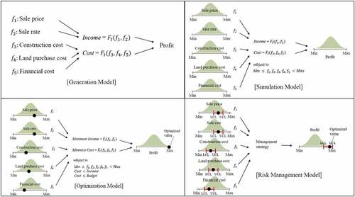
The risk factors will vary dynamically during the project cycle, from planning to construction to sales, which take several years until completion. Therefore, Lee et al. (2019) developed a dynamic simulation model for an apartment project, as shown in Figure 3. In this simulation model, each risk factor is defined as probabilistic random variables to represent the dynamic change of risk factors. As a result, the project profit is also reflected in probabilistic distribution. By this simulation model, the developer can observe the min-max value of risk factors, project profit, and all possible outcomes.

Next, to address risk analysis, an optimization model is developed. A study by Jang et al. (2019) developed an optimization model of residential houses in Korea. The optimization model is run multiple times to obtain the optimized value of project profit. Then, the value of risk factors corresponding to the optimum value of project profit is identified (Figure 3).

These previous studies have limitations as these papers had not considered the last step of risk management, i.e., risk response and control. There are uncertainties in the project due to changing economic conditions. The developer cannot just refer to the single point of optimum value of project profit and risk factors throughout apartment development. Therefore, this study aims to develop a risk management model of apartment development projects using system dynamics (Figure 3). The strategy presented in this paper is by setting the risk range limit (LCL and UCL) to the risk factors developed in a dynamic system. In this regard, the developer can achieve the optimum project profit if the risk factors are managed within the limit. Using this model, it is possible to concisely simulate the strategy and analyze whether the targeted optimum profit is achieved or not.

2.2. Monte Carlo method

The Monte Carlo method is a stochastic technique based on generated random numbers for any factor with inherent uncertainty to perform risk analysis (Tian 2006). It works by using different sets of random values of input variables from the probability functions resulting in a distribution of possible outcome values. The probability function, along with the mean and standard deviation, defines how likely certain risk factors will occur. Some standard probability distributions are normal, lognormal, uniform, and triangular. Monte Carlo simulation could involve hundreds of thousands of recalculation/iterations.

Another forecasting method is the Deterministic or “single-point estimate” method. The deterministic method uses a fixed value of input variables without randomness to determine the outcome with certainty (Renard, Alcolea, and Ginsbourger 2013). Each method has its strengths and weaknesses. The strengths of the Monte Carlo method are that it provides a much more comprehensive view of what may happen by considering all possible input variables and reflecting the likelihood that every situation will occur. The Monte Carlo method is particularly suitable for this study as the economic risk factors have high uncertainty characteristics with no fixed value and can be changed dynamically over time depending on the changing economic conditions.

2.3. System dynamics

System dynamics is an approach to understanding the nonlinear behavior of the complex system over time based on feedback systems (Sterman 2000). As implemented in the apartment development project, system dynamics grasp the feedback between variables and the dynamic change of the output according to the change of input variables (Kim et al. 2020).

System dynamics has two principal diagrams, i.e., causal loop and stock/flow diagrams (Sterman 2001). A causal loop diagram illustrates the causal relationship between key variables and how they are interconnected. The variables are represented as texts and the causal relationships between variables are represented as arrows. The arrows are labeled with “+” or “–” signs to identify the causal effects. “+” indicates positive correlation while “–” indicates negative correlation. After a causal loop diagram is established, a stock/diagram is developed to illustrate the algebraic expression of the system by distinguishing the variables that are stocks and those that area flows (Egilmez and Tatari 2012). Stock and flow are two different entities. Stock are entities that can accumulate or be reduced, while flows are entities that make stocks increase or decrease. These two diagrams are fundamental in system dynamics. Causal loop diagrams provide a general description of the system, are easy to understand and are a valuable communication tool to people with a little background in system dynamics. Meanwhile, stock/flow diagrams provide a comprehensive view of how the system works.

2.4. Dynamic probabilistic simulation

The dynamic probabilistic simulation method is a statistical method to analyze the causal relationship of project risks using a probability distribution. It combines two main concepts: system dynamics and the Monte Carlo method (Jang et al. 2019). This study applied dynamic probabilistic simulation. First, the causal loop diagram and stock/flow diagram were developed to illustrate the causal relationship between the economic risk factors and the profit. Then, the risk factors were conditioned by the determined probability distribution function and acted as input variables in the system dynamics model. Accordingly, the project profit as the final output is also reflected as a probability distribution. Finally, by running optimization and setting risk range limits to the risk factors, the risk management to apartment development is conducted.

3. Dynamic simulation model of apartment

3.1. Apartment development phase

This section shows an existing dynamic simulation model of apartments that was developed by Lee et al. (2019). The dynamic model can be simulated in the apartment business stage (t₀–t₃) as shown in Figure 4, and it can be operated flexibly according to the developer’s decision.

Figure 4. Simulation phase of economic feasibility (Lee et al. 2019).

The t₀ is the initial project review phase, where the developer carries out the economic feasibility analysis. In this phase, the developer surveys the value of risk factors and profit of similar projects in the neighboring region as a basis for its project. The developer also runs the simulation model of risk factors to check the possible optimum project profit and the worst case of loss that might happen. Furthermore, the developer sets the risk strategy by setting the risk range limits (LCL and UCL) to manage the profit in the next phase. If the project is profitable, the developer continues the process of land acquisition and preliminary construction contracts.

Between t₀ and t₁, the developer conducts land acquisition and processes preliminary construction contracts. Consequently, the land cost is fixed in t₁ because land acquisition has been made. Between t₁ and t₂, the developer reviews the project design from the initial planning, such as the number of buildings and housing units. This leads to the decision on construction cost in t₂. Finally, the developer starts the apartment sales and construction in t₂. In Korea, it is common for developers to start selling the apartment simultaneously with the construction process. In such a way, the developer only shows the apartment type and design to potential buyers. Before the sales start, the developer determines the final sales price by considering the fixed land and construction cost, the targeted project profit, and the market conditions.

After t₂, the developer continuously checks the actual income, sales ratio, and financial cost. Supposing there is a tendency for a low sales ratio resulting in low income and high financial cost with the attendant risk of business failure, the developer conducts t₃. In t₃, the overall flow of funds, risk factors, and changes in the business environment are evaluated. The developer might adjust the strategy by changing the sales prices to keep the optimum profit. While Figure 4 only shows the development phase to t₃, the strategy can be adjusted multiple times after confirming new sales ratio by generating t₄, t₅, …, and so on until the project is completed.

3.2. Generation model

According to Lee, Kim, and Suh (2013), there was a ranking of risk factors influencing the profit of apartment development projects. The result was obtained from qualitative experience of the experts in Korea that has been quantified using Fussy Delphi – Analytic Hierarchy Process (FD-AHP). The most important factors out of the risk factors, in order, were sales price, sales ratio, land cost, construction cost, and financial cost. Indirect risk factors were also identified among others such as adjacent regions, traffic environment, complex size, and brand preference. This study only considered the main risk factors by applying the causal relationship between the risk factors and project profit in a causal loop diagram, as shown in Figure 5 and developed by Lee et al. (2019). The indirect risk factors were not considered because these factors cannot be quantified and do not significantly affect the profit. Finally, the economic feasibility of apartment development projects is determined by project profit, calculated using project costs, financial cost, sales income, and financial income.

Figure 5. Causal-loop diagram (Lee et al. 2019).

3.2.1. Income model

The total income ($TI$), as shown in Formula (1), is the sum of the monthly sales income. Monthly sales income is calculated by multiplying the total sales amount ($TSA$) with the monthly sales ratio ($S{R}_m$) under the conditions of an installment payment system. The number of months from project commencement to completion ($m$) is limited to the time from project commencement to completion. The $TSA$, as shown in Formula (2), is calculated using unit apartment sales price ($UASP$), apartment area by type ($A{A}_i$), apartment unit by type ($A{U}_i$), unit commercial area sales price ($UCASP$), and commercial area ($CA$).

(1) $TI=\sum _{m=1}^{n}TSAxS{R}_m$(1)

(2) $TSA=\sum _{i=1}^l\left(A{A}_{i}xA{U}_{i}xUASP\right)+\left(CAxUCASP\right)$(2)

Total sales ratio ($TSR$), as shown in Formula (3), is the sum of the monthly sales ratio with a value that starts from 0 and cannot exceed 1.

(3) $\begin{array}{rl}& TSR=\sum _{m=1}^{n}S{R}_1+\dots +S{R}_n\\ & 0\le TSR\le 1\end{array}$(3)

3.2.2. Cost model

The total cost ($TC$), as shown in Formula (4), is calculated as the sum of monthly construction cost ($C{C}_m$), monthly land cost ($L{C}_m$), and other costs ($O{C}_m$).

(4) $TC=\sum _{m=1}^n\left(C{C}_m+L{C}_m+O{C}_m\right)$(4)

Monthly construction cost ($C{C}_m$), as shown in Formula (5), is calculated using unit construction cost ($UCC$), apartment unit by type ($A{U}_i$), apartment area by type ($A{A}_i$), commercial area ($CA$), and monthly construction cost payment ratio ($CCP{R}_m$).

(5) $C{C}_m=\left(\sum _{i=1}^l\left(A{A}_{i}xA{U}_{i}xUCC\right)+\left(CAxUCC\right)\right)xCCP{R}_m$(5)

Monthly land cost ($L{C}_m$), as shown in Formula (6), is computed using unit land cost ($ULC$), land area ($LA$), and monthly land cost payment ratio ($LCP{R}_m$).

(6) $L{C}_m=ULCxLAxLCP{R}_m$(6)

Other monthly costs ($O{C}_m$), as shown in Formula (7), are calculated using unit other costs ($UOC$), total floor area ($TFA$), and monthly other costs payment ratio ($OCP{R}_m$).

(7) $O{C}_m=UOCxTFAxOCP{R}_m$(7)

3.2.3. Financial Cost Model

The total financial cost ($TFC$), as shown in Formula (8), incorporates monthly financial income and monthly financial cost.

(8) $\begin{array}{rl}& TFC=\sum _{m=1}^n\left(I_m-C_m\right)\times IR\\ & IR:\left\{\begin{array}{c}if{I}_m-C_m\ge 0,depositinterestratesisapplied\\ if{I}_m-C_m<0,loaninterestratesisapplied\end{array}\right\}\end{array}$(8)

Monthly financial cost ($F{C}_m$), as shown in Formula (9), occurs when the monthly cost ($C_m$) is greater than monthly income ($I_m$). It is calculated by applying loan interest rates ($I{R}_{loan}$).

(9) $F{C}_m=\left(C_m-I_m\right)\times I{R}_{loan}$(9)

Monthly financial income ($F{I}_m$), as shown in Formula (10), occurs when monthly income ($I_m$) is greater than monthly cost ($C_m$). It is calculated by applying deposit interest rates ($I{R}_{deposit}$).

(10) $F{I}_m=\left(I_m-C_m\right)\times I{R}_{deposit}$(10)

3.2.4. Project Profit Model

Project profit ($PP$), as shown in Formula (11), is calculated using monthly income ($I_m$), monthly financial income ($F{I}_m$), monthly cost ($C_m$), and monthly financial cost ($F{C}_m$).

(11) $PP=\sum _{m=1}^n\left\{\left(I_m+F{I}_m\right)-\left(C_m+F{C}_m\right)\right\}$(11)

3.3. Simulation model

As shown in Figure 6, the simulation model comprises the income, cost, financial, and profit simulation models. The income simulation model calculates monthly income over a sales period based on unit sales price, sales ratio, and installment payment system. The cost simulation model calculates the monthly cost over the project period on the basis of construction, land, and other costs. The financial cost simulation model calculates the monthly financial cost or income depending on monthly cost and income. These models are integrated into one simulation model that calculates project profit and ROR, as shown in Figure 7.

Figure 6. Income, cost, financial cost, and project profit model.

Figure 7. Integrated simulation model.

The software used to build the simulation model is Powersim Studio 10 (Powersim Software AS, 2014). It is a simulation software for forecasting and analysis of complex dynamic problems. Some functions available in PowerSim Studio, among others: (1) build and run System Dynamics models, (2) run scenarios, Monte Carlo simulation, and include uncertainty for input factors, and (3) conduct risk analysis, optimization, and risk management.

4. Analysis of risk range limit of risk factors

4.1. Sales price

Generally, apartment sales prices are determined by the economic condition. Factors affecting the market situation are supply and demand, government policy, urbanization rate, and population growth (Jiang 2012). These factors are observed from three main economic periods that affected house prices in Korea: housing market expansion from 1988 to 1990, foreign exchange crisis from 1997 to 1999, and global financial crisis from 2008 to 2009 (Kim, Kim, and Kim 2016).

In the first period (1988–1990), Korea achieved rapid economic growth. Consequently, the urban population increased, creating a high demand for apartments and increased apartment transactions. The whole housing market maintained a stable trend until 1996 when the foreign exchange crisis occurred. In the second period (1997–1999), the apartment transaction market was depressed because of the economic recession. Eventually, from 2004, apartment prices recovered. In the third period, a global financial crisis in 2008 resulted in depression in the apartment transaction market.

Presently, Korea faces the COVID-19 crisis as do other countries. Many countries, including Korea, have expanded liquidity and cut interest rates to overcome the economic downturn caused by COVID-19. Since liquidity expansion lowers the value of money and interest rate cuts stimulate the expansion of borrowing, people are more inclined to invest in assets at this time. Consequently, house prices rise for the most significant portion of asset investment. It has been confirmed that despite the economic downturn, abundant liquidity, and low interest rates can lead to a rise in house prices.

It can be concluded that apartment house prices fluctuated, as shown in Figure 8. The apartment sales price fluctuates according to the line of per capita national income (Figure 8(a). Figure 8(b) shows the ①–④ fluctuation cycle of Figure 7(a) as a circle. For reference, as a result of analyzing data for the past 50 years in Korea, it is confirmed that the housing market fluctuates with a cycle of approximately 10–12 years.

Figure 8. Fluctuation of apartment house prices in Korea: (a) Apartment house prices vs. Per capita national income. (b) Apartment house price cycle.

The developer must understand the apartment house price cycle to establish a strategy for developing apartments and setting the unit sales price. In this study, the unit sales price is represented in USD/m². The risk range limit (LCL and UCL) of unit sales price must be determined after checking the housing price in the neighboring regions and economic trend when selling the housing unit, and three risk range limits can be set as shown in Figure 8. For reference, in Figure 9, the minimum and maximum risk range limits are developed in conjunction with the minimum and maximum profit, respectively.

Figure 9. Risk range limit cases of the unit sales price.

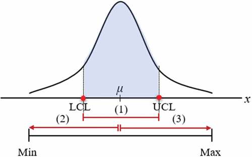
1. Case (1) is a general case, and as shown in Figure 8, the UCL and LCL of the unit sales price are set as the risk range limit. For example, ±10% of the average house price near the project site are set to UCL and LCL, respectively. The UCL and LCL can be adjusted, considering the profit limit.

2. Case (2) is a case where the sales price is set at the peak stage, and the unit sales price is highly likely to be set at this point. Thus, the risk range limit in Figure 8 should reflect the situation in which the economy goes down after the peak (①) and reaches a recession (③). In this section, the prices of neighboring houses fall, and accordingly, the unit sales price may fall beyond the minimum profit to a level that causes severe losses. In this case, the UCL is the starting point at the right end of the arrow in case (2), and the LCL may exceed the minimum risk range limit. Hence, before the minimum risk range limit is exceeded, the project developer must make a strategic decision on whether to continue the project.

3. Case (3) is a case where the sales price is set in the recession phase, and at this point, the sales price is highly likely to be set low. Therefore, the risk range limit in Figure 8 should reflect the situation in which the economy rises after a recession (③) and reaches a peak (①). In this section, the price of neighboring houses rises, and accordingly, the sales price may exceed the maximum profit. In this case, the LCL is the starting point at the left end of the arrow in case (3), and the UCL may exceed the maximum risk range limit.

As shown in Figure 8, the housing market should be predicted through time series analysis to set a reasonable risk range limit in the above three cases. In Korea, an apartment building development project takes at least 3–5 years from land acquisition, design, sale, and construction to completion, so the business cycle should be analyzed. The analysis result should be set as the risk range limit of the unit sales price.

4.2. Sales ratio

The sales ratio is directly related to the sale price (Lee et al. 2019). Generally, the higher the sale price, the lower the sales ratio. Even if a small number of housing units are sold in a high-rise apartment building project, the entire building must be constructed. The reason is that the buyer’s housing units are distributed in various parts of the building, and the building must be completed on time (Lee et al. 2019).

For example, in an apartment building of 1,000 units, all units must be built even if only 50 units have been sold. It is impossible to pay monthly construction progress payments and financial cost in this case. Moreover, the financing cost for land, construction, and other costs are high, so the project profit is relatively reduced. However, if the apartment units are completely sold out at the beginning of the sale, it can be interpreted as a lost opportunity to sell at a higher sales price. Consequently, developers lose the chance to make more profits.

A study conducted by Son et al. (2019) attempted a regression model to forecast the initial sales ratio by analyzing 15 apartment projects’ data in Korea. It was found that the smaller the difference between average unit sales price to the surrounding market price, the higher the sales ratio. However, there has been no mathematical formula to explain the dynamic relationship between sales ratio and unit sales price.

Thus, in this study, the sales ratio has been determined before the simulation by considering the experts’ judgment, sales ratio of similar projects in the neighboring region, the economic condition, and the target of sales ratio set by the developer. To increase the sales ratio, the developer attempts to set the unit sales prices as close as possible to the average unit sales price in the surrounding area.

4.3. Construction cost

Construction cost has a high contribution to the total cost of the apartment project. It comprises material, equipment, labor, and overhead costs (Park et al. 2012). Consequently, the price fluctuation of material, equipment, and labor highly influences overall construction cost. The developer has to consider the inflation that may increase the construction cost and make sure the affected construction cost remains reasonable so that the targeted profit is reached. Thus, this study proposes a strategy by setting a risk range limit of construction cost.

In the initial project review stage (t₀), the developer sets the initial construction cost by calculating the construction cost of the project itself and checking the construction cost of similar projects in the surrounding area. Then, the developer sets the maximum construction cost (UCL) that the project can endure after considering the inflation and can still generate targeted profit. Finally, the developer sets the minimum construction cost (LCL) that can happen. For example, although it rarely happens, the developer decides to change the project’s design. Accordingly, the developer builds fewer apartment buildings than initially planned which causes lower construction cost (LCL). For example, the UCL and UCL of the construction cost are assumed to be ±10% of the initial construction cost.

4.4. Land cost

Land cost contributes a significant proportion to the total project cost. In Korea, a developer deals with two land purchase conditions when securing land to develop an apartment project. Generally, an apartment project needs a large area of land. In some cases, supported by government policy, the government provides large lots in the outskirts of the city that developers can buy. However, in some cases, the developer must buy several small lots owned by different landowners and combine the lots to gain enough area to build apartments. When purchasing many small lots, the developer deals with many landowners who have various requirements and request different land prices. Some landowners may insist on selling their land higher than the average land price.

In the initial project review stage (t₀), the developer has set the initial land cost by surveying the surrounding area and considering the business and economic condition. Then, the developer forecast the risk range limit by considering two land purchase conditions. For example, buying some big lots set as −10% of the initial land cost is the LCL. Meanwhile, purchasing many small lots set as +10% of the initial land price is the UCL.

4.5. Financial cost

The financial cost is calculated by subtracting a monthly financial cost from monthly financial income. It occurs from project commencement to sales completion and depends on the sales price, sales ratio, construction cost, and land cost. The financial cost will increase sharply when the building construction is completed, but with a low sales ratio. The sales income is insufficient to cover the cost, whereas the project loan calculated using loan interest rate steadily increases. Thus, it is crucial to set the risk range limit of financial cost by considering the business environment and the developer’s ability to raise funds to cover the financial cost on time.

The financial cost is highly influenced by the combination of sales price, sales ratio, construction cost, land cost, and the sales period of the apartment. Thus, it is essential to set the sales price, construction cost, and land cost at their optimum value and reach a 100% sales ratio as early as possible to reduce the financial cost.

5. Case application and discussion

This section validates the developed simulation model through case application by running the simulation model in each phase of the apartment development project (t₀–t₃). The developer sets risk range limits to risk factors such as sales price, land cost, and construction cost to maintain the optimum profit. The risk range limit can be changed dynamically depending on the current economic conditions to achieve the optimum profit.

Table 1 shows an overview of the case project. The project comprises 335 apartment units (two types) and a commercial area of 16,048 m². There are two types of apartment units: 167 units of 84 m² type A and 168 units of 84 m² type B. The total land, the building area, and the total floor area are 6,441, 6,292, and 75,359, respectively.

Table 1. Overview of the apartment case project.

Item	Initial value	Unit
Land area	6,441	m^2
Total floor area	75,359	m^2
Building area	6,292	m^2
Commercial area	16,048	m^2
Apartment sales price	3,910	USD/m^2
Commercial area sales price	6,368	USD/m^2
Land cost	7,998	USD/m^2
Construction cost	1,242	USD/m^2
Other costs	937	USD/m^2
Loan interest rates	4.1	%/year
Deposit interest rate	1.28	%/year
Project period	60 (1^st–60^th)	months
Land acquisition period	18 (1^st–18^th)	months
Construction period	42 (19^th–60^th)	months
Apartment unit 84A m^2 Apartment unit 84B m^2	167 168	unit

The initial economic risk factors were set as follows. The apartment sales price and commercial area sales price were set as 3,910 and 6,368 USD/m², respectively. The land, construction, and other costs were set as 7,998, 1,242, and 937 USD/m², respectively. Loan interest rates of 4.1%/year and 2.9%/year for deposit interest rates were applied. The project period was 60 months of which the land acquisition period lasted for 18 months (1^st–18^th months), and the construction period lasted for 42 months (19^th–60^th months). The developer expected a 100% sales ratio, meaning the apartment units and commercial area are sold out within a targeted 12 months after the sales start (19^th–30^th months).

5.1. Forecasting simulation at initial stage review (t₀)

The simulation was set as shown in Figure 5. Sales price, land cost, and construction cost were conditioned by normal distribution function and used as input variables. The initial value of each risk factor was set as the mean, and 0.1 was used as the standard deviation of the function. The sales ratio was 100% as the developer aimed for a sold-out apartment unit and commercial area. The initial three-month sales were set to 60% by considering the sales ratio result of similar and successful projects in the neighboring region.

The optimization was performed by running the simulation 10,000 times. Accordingly, the profit as final output was also reflected as probability normal distribution. Figure 10 shows the random variable generation by risk factors and project profit, and Table 2 shows the simulation result. The profit varied from −29,285,821 USD to 94,408,987 USD. By dividing profit by total cost and multiplying by 100%, the average ROR was 20%.

Figure 10. Random variable generation by risk factors and project profit.

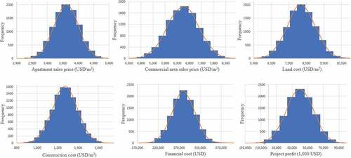
Table 2. Result of forecasting simulation.

Item	Average	Maximum	Minimum
Apartment sales price (USD/m^2)	3,910	5,337	2,350
Commercial sales price (USD/m^2)	6,368	8,463	3,741
Land cost (USD/m^2)	7,998	11,470	5,037
Construction cost (USD/m^2)	1,242	1,704	779
Financial cost (USD)	272,636	394,877	167,726
Profit (USD)	34,959,587	94,408,987	−29,285,821
Rate of return (%)	20%	58%	−14%

KRW 1,177.00 = USD 1.00 as of 2021/12/12 (Bank of Korea).

In Korea, the usual ROR of apartment projects is 9%–12%. However, this project obtains the average ROR as high as 20% due to low initial land cost and high initial sales price. Expecting this project to go well, the optimum ROR set in this study was 30%. Consequently, the optimum profit was 52,251,666 USD with ROR 30%. The value of independent variables corresponding to optimum profit was 4,232 USD/m² for the apartment sales price, 6,731 USD/m² for the commercial area sales price, 7,920 USD/m² for land cost, and 1,120 USD/m² for construction cost. Combining these sales prices, construction cost, and land cost resulted in 250,582 USD for financial cost.

This study set the UCL and LCL to control the risk factors and manage the optimum profit, which is ±10% of the risk factors, as shown in Table 3. By setting the targeted ROR to 27%–33% (±10% of optimum ROR), the apartment sales price, commercial sales price, land cost, construction cost, and financial cost must be set within the ranges of 3,809–4,655 USD/m², 6,058–7,404 USD/m², 7,128–8,712 USD/m², 1,008–1,232 USD/m², and 225,524–275,640 USD, respectively, as shown in Table 3 and Figure 11. Supposing they are beyond these control limits due to changes in economic conditions; a risk strategy adjustment is made by rerunning the simulation resulting in new optimum profit and new risk range limit of risk factors. The developer refers to these new results until changes in the business environment occur again.

Figure 11. Setting risk range limit to risk factors and project profit.

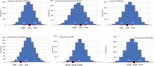
Table 3. Setting risk range limit to risk factors at initial stage review (t₀).

Description	Apartment sales price (USD/m^2)	Commercial area sales price (USD/m^2)	Land cost (USD/m^2)	Construction cost (USD/m^2)	Financial cost (USD)
LCL	3,809	6,058	7,128	1,008	225,524
Risk factors of optimum profit	4,232	6,731	7,920	1,120	250,582
UCL	4,655	7,404	8,712	1,232	275,640

5.2. Resimulation during land acquisition to fixation of land cost at t₁

During this phase, the business environment changes dynamically, which is different from what the developer expected in the forecasting simulation. In this phase, the developer attempts to secure land. Initially, purchasing big lots provided by the government is the quickest and cheapest way. However, the land offered by the government is limited. In some cases, the developer has to secure land by buying small lots owned by many private owners. The process of acquiring small lots and combining them into big lots requires more time and higher costs than initially planned, which also causes the risk to the developer.

Although the developer initially expects low land cost by buying big lots provided by the government, this study assumes the developer buys small lots, causing the land cost to increase 10% higher than the initial land cost. The simulation was rerun to search for an optimum profit with a fixed land cost of 8,798 USD/m². Consequently, the average profit was 29,967,753 USD (ROR 16%), which was 4% lower than the average ROR in the forecasting simulation.

If the developer sets the ROR at 27%–33%, there is a significant increase in the sales price, which is not favorable for the developer. Thus, the risk strategy implemented in this phase was done by decreasing the optimum ROR to 26%, resulting in an optimum profit of 46,084,768 USD. The value of independent variables corresponding to optimum profit was 4,128 USD/m² for the apartment sales price, 6,569 USD/m² for the commercial area sales price, 1,086 USD/m² for construction cost, and 264,540 USD for financial cost. Accordingly, the targeted ROR changed to 23.4%–28.6% (±10% of optimum ROR). As shown in Table 4, the new risk range limit of risk factors corresponding to the new targeted ROR was 3,715–4,541 USD/m² for the apartment sales price, 5,912–6,569 USD/m² for the commercial area sales price, 975–1,195 USD/m² for construction cost, and 238,086–290,994 USD for financial cost.

Table 4. Risk range limit to risk factors after land cost is fixed (t₁).

Description	Apartment sales price (USD/m^2)	Commercial area sales price (USD/m^2)	Construction cost (USD/m^2)	Financial cost (USD)
LCL	3,725	5,912	977	238,086
Risk factors of optimum profit	4,128	6,569	1,086	276,961
UCL	4,540	7,226	1,194	290,994

5.3. Resimulation during the finalization of the construction contract to the fixation of the construction cost at t₂

During this phase, the developer had bought land at 8,798 USD/m² resulting in the developer focusing on the fixation of the construction contract. The developer has to produce an optimal design that comprehensively considers both cost and schedule while satisfying the owner’s requirements. Reckless planning can result in cost overrun and schedule overrun. When there is a construction delay, the cost of materials/services increases, causing higher financial cost.

This study assumes the construction cost increases 10% higher than the initial construction cost after considering the inflation of materials/services price. The simulation was rerun to search for the optimum profit with construction cost fixed at 1,366 USD/m². After running the simulation 10.000 times, the average profit was 24,404,006 USD (ROR 13%).

By still setting the optimum ROR 26%, the optimum profit was 48,083,728 USD. The value of apartment sales price, commercial area sales price, and financial cost corresponding to optimum profit were 4,460 USD/m², 6,885 USD/m², and 276,961 USD, respectively. As the targeted ROR was set to 23.4%–28.6%, the new risk range limit of apartment sales price, commercial sales price, and financial cost was 4,014–4,906 USD/m², 6,197–7,574 USD/m², 249,265–304,657 USD, respectively (Table 5).

Table 5. Risk range limit to risk factors after construction cost is fixed (t₂).

Description	Apartment sales price (USD/m^2)	Commercial area sales price (USD/m^2)	Financial cost (USD)
LCL	4,014	6,197	249,265
Risk factors of optimum profit	4,460	6,885	276,961
UCL	4,906	7,554	304,657

5.3. Resimulation after confirming actual sales ratio at t₃

At the start of this phase, the apartment unit and commercial area are sold at 4,460 and 6,885 USD/m², respectively. The monthly actual sales ratio is observed, which may differ from the target in the forecasting simulation at t₀.

This study developed two scenarios according to sales price fluctuation, as shown in Figure 7. The first scenario is defined as when the economic condition rises after a recession and reaches a peak stage. By contrast, the second scenario is established when the economy’s condition falls from peak stage to recession, causing a low sales ratio.

The first scenario assumes a 60% sales ratio is achieved in the initial 3 months of sales. By observing good economic conditions, the developer recognizes that the project can gain more profit, and the developer does not want to lose this opportunity. Suppose the current sales price is kept as it is; the optimum profit is 48,083,728 USD with ROR 26%. The developer decides to increase the targeted ROR to 28.6%. Based on the optimization result, the apartment and commercial sales prices are increased to 4,730 and 7,320 USD/m².

The second scenario assumes the developer obtains a 30% sales ratio after 3 months of sales, which were only 50% from the target. After observing the business environment, the economic condition is worsened from peak stage to recession resulting in low purchasing power on the part of potential buyers. Supposing the developer still set the apartment sales price at 4,460 USD/m² and the commercial area sales price at 6,885 USD/m²; the optimum profit is not achieved, and the apartment project fails. Furthermore, the financial cost increases to 526,065 USD maximum, which is many times higher than the financial cost set in the risk range limit.

After checking similar projects in the neighboring region, the developer decides to lower the sales price by 5%, so the apartment and commercial sales prices are set to 4,237 and 6,541 USD/m², respectively. The developer set the target for the apartment to be sold out in 1 year. The simulation showed an optimum profit of 35,028,938 USD with an ROR of 19%, and the financial cost was 299,961 USD, which is within the risk range limit. Although the ROR decreased from 26% to 19%, the developer gains profit and avoids a severe loss.

Assuming that the actual sale ratio for the next month fails to achieve the expected sale ratio, the developer might set t₄ to evaluate the cash flow and establish a new strategy by adjusting the risk range limit of the sales price or setting a new reasonable target profit. This process strategy adjustment can be conducted many times until project completion.

In this way, the model developed based on system dynamics offers significant advantages. First, the model can logically correspond to the dynamic change of risks arising as the project progresses, from the planning stage in t0, where risk factors are varied, to the next stages where one by one of the risk factors become a fixed factor. The risk range limit of risk factors at each phase can secure the optimum profit of the project. Other than that, the model becomes a strategic communication tool within the developer to make informed decisions. However, the model also has some weaknesses that need to be addressed. First, the model can be optimized depending on the developer’s analysis and response abilities, especially in understanding the changing business environment. This study only illustrated apartment development from t₀ to t₃, where new risk range limits were set in each stage according to economic conditions. While in fact, the strategy adjustment can be conducted many more times after t₃ until project completion. Besides that, after running the risk management model in each stage, the developer will need time to implement the changes value of risk factors as it involves many parties within the developer.

6. Conclusion

This study developed a risk management model that can dynamically forecast, control, and manage an apartment development project’s economic risk factor based on a system dynamics simulation model. The risk management was applied by setting a risk range control limit (LCL and UCL) to risk factors to maintain optimum profit. The simulation model was verified through case application throughout the apartment development phase (t₀–t₃) as shown in the following.

The first simulation was conducted at the initial stage review (t₀) as a forecasting simulation. After running the simulation 10,000 times using probability distribution to each risk factor, the optimum profit was 52,251,666 USD with ROR 30%. The value of independent variables corresponding to optimum profit was 4,232 USD/m² for the apartment sales price, 6,731 USD/m² for the commercial area sales price, 7,920 USD/m² for land cost, and 1,120 USD/m² for construction cost. By setting the targeted ROR to 27%–33% (±10% of optimum ROR), the apartment sales price, commercial sales price, land cost, and construction cost must be set within the ranges of 3,809–4,655, 6,058–7,404, 7,128–8,712, and 1,008–1,232 USD/m².

Throughout the development phase, the land cost was fixed in t₁, and the construction cost was fixed in t₂. Due to these changes, a risk strategy adjustment is made by rerunning the simulation resulting in new optimum profit and new risk range limit of risk factors. The risk strategy implemented in t₁ decreases the optimum ROR to 26%, resulting in an optimum profit of 46,084,768 USD. The new risk range limit of risk factors corresponding to a new targeted ROR (23.4%–28.6%) were 3,715–4,541 USD/m² for apartment sales price, 5,912–6,569 USD/m² for commercial area sales price, 975–1,195 USD/m² for construction cost, and 238,086–290,994 USD for financial cost. A similar strategy was implemented in t₂.

Finally, two scenarios were developed in t₃. The first scenario assumed that a 60% sales ratio is achieved in the initial 3 months of sales. The developer increased the target of ROR to 28.6% to gain more profit. Based on the optimization result, the apartment and commercial area sales prices were increased to 4,730 and 7,320 USD/m². The second scenario assumed the developer obtains a 30% sales ratio after 3 months. The developer decided to decrease the sales where apartment and commercial sales prices were set to 4,237 and 6,541 USD/m², respectively. The simulation showed an optimum profit of 35,028,938 USD with a ROR of 19%.

The developer might set t₄ in case the actual sales ratio for the next month fails to achieve the target. In t₄, the developer establishes a new strategy by adjusting the risk range limit of the sales price in accordance with the new reasonable target profit/ROR. The developer might set t₄, t₅, …, and so on, a few times until the project is completed. In this way, the model can logically correspond to the dynamic change of risks arising as the project progresses. The risk range limit assists the developer in maintaining optimum profit and making quick and informed decisions over the changing business environment. Furthermore, the model becomes a strategic communication tool within the developer to make quick and informed decisions. However, it needs to be emphasized that the success of the model’s usage depends on the developer’s analysis and response abilities, especially in understanding the changing business environment.

Notations

Variables and functions

$TI=Totalincome\left(USD\right)$

$TSA=Totalsalesamount\left(USD\right)$

$S{R}_m=Salesratiopermonth$

$A{A}_i=Apartmentareapertype\left(m^2\right)$

$A{U}_i=Apartmentunitpertype$

$UASP=Unitapartmentsalesprice\left(\frac{USD}{m^2}\right)$

$CA=Commercialarea\left(m^2\right)$

$UCASP=Commercialareasalesprice\left(\frac{USD}{m^2}\right)$

$TSR=Totalsalesratio$

$TC=Totalcost\left(USD\right)$

$C{C}_m=Monthlyconstructioncost\left(USD\right)$

$L{C}_m=Monthlylandcost\left(USD\right)$

$O{C}_m=Monthlyothercosts\left(USD\right)$

$UCC=Unitconstructioncost\left(\frac{USD}{m^2}\right)$

$CCP{R}_m=Constructioncostpaymentratiopermonth$

$ULC=Unitlandcost\left(\frac{USD}{m^2}\right)$

$LA=Landarea\left(m^2\right)$

$LCP{R}_j=Landcostpaymentratiopermonth$

$UOC=Unitofothercosts\left(USD\right)$

$TFA=Totalfloorarea\left(m^2\right)$

$OCP{R}_m=Othercostspaymentratiopermonth$

$TFC=Totalfinancialcost\left(USD\right)$

$F{C}_m=Monthlyfinancialcost\left(USD\right)$

$F{I}_m=Monthlyfinancialincome\left(USD\right)$

$C_m=Monthlycost\left(USD\right)$

$I_m=Monthlyincome\left(USD\right)$

$I{R}_{loan}=Loaninterestrates\left(\mathrm{\%}\right)$

$I{R}_{deposit}=Depositinterestrates\left(\mathrm{\%}\right)$

$PP=Projectprofit\left(USD\right)$

Disclosure statement

No potential conflict of interest was reported by the author(s).

Additional information

Funding

This work was supported by the National Research Foundation of Korea (NRF) grant funded by the Korea government (MOE) (No. 2017R1D1A1B04033761;2022R1A2C2005276).

Notes on contributors

Titi Sari Nurul Rachmawati

Titi Sari Nurul Rachmawati is studying in architectural engineering from Kyung Hee University, as a student of doctoral course. She studied Civil Engineering at civil engineering department, Universitas Indonesia. After that, she finished master’s degree in environmental engineering and sustainable infrastructure at KTH Royal Institute of Technology, Sweden. She is actively conducting research on simulation, optimization, and risk management of building projects.

Sunkuk Kim

Sunkuk Kim studied Construction Engineering and Management at the department of architectural engineering, Seoul National University in Korea. He had joined three Korean construction firms for 12 years. He conducted research at the department of civil engineering, Stanford University from 1994 to 1995 as a visiting scholar. Since September 1995, he has served at Kyung Hee University as a professor. He has concentrated on the research such as health performance evaluation of buildings, development of sustainable construction technology and management, simulation, optimization and risk management, and construction information technology. Especially, for about a decade, he has participated in the development of SMART frame, a sustainable structural system, and production technology of free-form concrete panels.

References

- Egilmez, G., and O. Tatari. 2012. “A Dynamic Modeling Approach to Highway Sustainability: Strategies to Reduce Overall Impact.” Transportation Research Part A 46 (7): 1086–1096. doi:10.1016/j.tra.2012.04.011.
- Gehner, E. 2008. Knowingly Taking Risk Investment Decision Making in Real Estate Development. Delft: Eburon Academic Publishers.
- Hwang, M., J. Quigley, and J. Son. 2006. “The Dividend Pricing Model: New Evidence from the Korean Housing Market.” The Journal of Real Estate Finance and Economics 32 (3): 205–228. doi:10.1007/s11146-006-6798-3.
- Jang, J., S. Ha, K. Son, and S. Son. 2019. “Financial Analysis Model Development by Applying Optimization Method in Residential Officetel.” Journal Korea Institute of Building Construction 19 (1): 067–076. doi:10.5345/JKIBC.2019.19.1.067.
- Jiang, F. 2012. “The Study of the Relationship between House Price and Price Tolerance in China from the Perspective of Systems Engineering.” Systems Engineering Procedia 5: 74–80. doi:10.1016/j.sepro.2012.04.012.
- Kim, S., J. Kim, and J. Kim. 2016. “Structural Changes in the Korean Housing Market before and after Macroeconomic Fluctuations.” Sustainability 8 (5): 415. doi:10.3390/su8050415.
- Kim, J., K. Son, J. Jang, and S. Son. 2020. “Development of an Income and Cost Simulation Model for Studio Apartment Using Probabilistic Estimation.” Journal of Asian Architecture and Building Engineering 20 (5): 546–555. doi:10.1080/13467581.2020.1800474.
- Kim, S. 2020. “Modeling Concept for Problem-Solving.”
- Lee, S., S. Kim, and S. Suh. 2013. “Analysis of the Risk Influence Factors in Apartment Building Development Projects.” Journal of the Korea Institute of Building Construction 13 (4): 424–433. doi:10.5345/JKIBC.2013.13.4.424.
- Lee, K., S. Son, D. Kim, and S. Kim. 2019. “A Dynamic Simulation Model for Economic Feasibility of Apartment Development Projects.” International Journal of Strategic Property Management 23 (5): 305–316. doi:10.3846/ijspm.2019.9822.
- Nnamani, O. C., 2018. “Application of Risk Management Techniques in Property Development Projects in Nigeria: A Review.” 25th European Real Estate Society Conference, Reading, United Kingdom.
- Park, W., T. Kang, S. Baek, and Y. Lee. 2012. “Analysis of Construction Cost Fluctuation Trends and Features on Apartment Housing.” Journal Korea Institute of Building Construction 12 (6): 624–635. doi:10.5345/jkibc.2012.12.6.624.
- Park, J. Y. 2018. “System Development for Risk Management of Apartment Building Projects using system dynamics.” ( Ph.D. thesis). Kyunggido: Kyunghee University
- Powersim Software AS. 2014. “Powersim Studio 10.” [Computer software]. https://powersim.com/
- Project Management Institute. 2013. A Guide to the Project Management Body of Knowledge 5th Eds. Pennsylvania: Project Management Institute, Inc.
- Renard, P., A. Alcolea, and D. Ginsbourger. 2013. “Stochastic versus Deterministic Approaches.” Environmental Modelling 133–149. doi:10.1002/9781118351475.ch8.
- Shin, E., S. Hong, and S. Kim. 2016. “Changes in Public Perceptions of Apartments: Television and Newspaper Advertisements, 1960–2010.” Journal of Asian Architecture and Building Engineering 15 (1): 65–72. doi:10.3130/jaabe.15.65.
- Son, S., and S. Kim. 2019. “A Regression Model for Forecasting the Initial Sales Ratio of Apartment Building Projects.” Journal Korea Institute Building Construction 19 (5): 439–448. doi:10.5345/JKIBC.2019.19.5.439.
- Sterman, J. 2000. Business Dynamics: Systems Thinking and Modeling for a Complex World. Boston: McGraw-Hill Education.
- Sterman, J. 2001. “System Dynamics Modeling: Tools for Learning in a Complex World.” California Management Review 43 (4): 8–25. doi:10.2307/41166098.
- Tanzil, A., M. Setiadi, and I. Santoso. 2018. “Risk Analysis of Apartment Project Development.” International Journal of Innovative Research in Science, Engineering and Technology 7 (9): 9396–9405. doi:10.15680/IJIRSET.2018.0709013.
- Tian, Y., 2006. “The Application of Simulation to Project Evaluation for Real Estate Developers in China.” ( Masters diss.). United States: Massachusetts Institute of Technology.
- Won, I. W. 2014. “An Investment Risk Management Model of Apartment Building Projects using System Dynamics Techniques.” ( Ph.D. thesis). Kyunggido: Kyunghee University.