Undamped non-linear vibration mechanism of bolted flange joint under transverse load

ABSTRACT

Bolted flange joints are commonly utilized in engineering constructions; nevertheless, their dynamic behavior is complicated when nonlinearity is present. The bolted flange joint structure in this research is considered as a spring-mass system, and the equivalent axial two bi-linear springs-bending beam model, as well as the system’s vibration control equation, is created to examine the joint structure’s vibration characteristics under transverse stress. The results indicate that when the spring stiffness is constant and the stiffness is a linear function of displacement, and the mass matrix of the vibration control equation is coupled, the system produces only transverse vibration upon transverse impact; when the spring axial stiffness is a linear function of displacement and the mass matrix of the vibration control equation is not coupled, the spring stiffness is bilinear and the stiffness is a quadratic function of displacement, the system will vibrate transversely and longitudinally under the transverse impact. Regardless of how the spring stiffness is simplified, the system’s transverse or transverse and axial movement is a stable periodic vibration with a vibration response proportional to the system’s mass and the radius L of the connected cylindrical shell.

KEYWORDS:

• Bolt connection
• bolted flange joint
• transverse load
• nonlinear dynamics
• vibration mechanism

1. Introduction

Bolted flange joint connection is an efficient and removable combination structure with the advantages of good operability and simple structure (Pereira, Mantelli, and Milanez 2008), which is widely used in industrial mechanical structures such as aerospace and petrochemical industries (He 2015). Bolted flange joints usually have good strength and stiffness (Pereira, Mantelli, and Milanez 2008; de Lima et al. 2009; Lehnhoff, Ko, and McKay 1994), but their reliability can be affected by the number of bolts, bolt preload, and fatigue of the connection parts (Zhang 2003; Wang, Li, and Huang 2006; X, S, and Ma et al. 2019).

The nonlinear static properties of the bolted flange joint are generally studied using contact algorithms of finite element models (Takaki and Fukuoka 2003; Abid 2008) and detailed analytical methods (Nassar 2009), and the related research methods are well established. For the dynamic properties of the bolted flange joint, a generally applicable established nonlinear dynamic research method has not been established due to the influence of various nonlinear factors such as gasket material nonlinearity, contact nonlinearity of each component, and load (He 2015; Yin 2008; T, R, and L et al. 2014). The current study of nonlinear dynamics of bolted joint assembly structures has been carried out mainly at two levels, macroscopic and microscopic. The macroscopic level is the simplification of the connection part of the structure, such as modeling the bolted structure as a linear spring-damper (Butner, Adams, and Foley 2012), a connection layer (Ahmadian et al., 2002), or a universal element (Ahmadian and Jalali 2007). The microscopic level (Hoang et al. 2021; Gia Ninh, Ngoc Viet Hoang, and Le Huy 2021) is mainly used to explain and analyze the mechanical properties by studying the physical mechanism of the micro-convex body contact deformation at the mechanical bonding surfaces between the components of the bolted flange joint.

Luan Yu et al (Luan 2012; Luan et al. 2013) studied and verified the static stiffness characteristics and dynamic response characteristics of the bolted combined structure by simplifying it into a beam unit structure model. Chen Hongwei et al (Chen and He et al. 2018) equated the combined joint part as a beam-spring and investigated the effect of bolt preload force and part geometry on the nonlinear characteristics of axial stiffness in the combined structure with different material shims. The above study explored an important characteristic of the bolted flange joint structure is the axial tensile and compressive stiffness nonlinearity, but the study of the mechanism of the generation of this nonlinear stiffness and the influencing factors is far from sufficient.

To study the impact response mechanism of the bolted combination structure under different approximate simplified conditions of transverse stiffness, this paper establishes a mass-spring system based on the literature (Chen and He et al. 2018) to study and analyze the nonlinear dynamical response mechanism of the combination structure and conduct experimental verification.

2. The equivalent axial two bi-linear springs-bending beam model

Luan (2012) investigated the axial nonlinear stiffness of bolted flange joint using the nonlinear static finite element approach. The study established that the bolted flange joint’s axial stiffness exhibits evident bilinear features. To further elucidate the relationship between the axial nonlinear stiffness of the bolt connection part and the overall axial nonlinear stiffness of the bolted flange joint, and to facilitate discussion of the effect of various design elements on the axial nonlinear stiffness of the connection part of the bolted flange joint, this paper approximates the bolt connection part of the piece connection bolted flange joint to the static analysis model of the two bi-linear springs-bending beams.

2.1. Establishment of the equivalent axial two bi-linear springs-bending beam model

To be able to express the axial stiffness characteristics of the bolted flange joint structure with an analytical expression based on the deformation characteristics of the bolt connection part under axial tension and compression loads, the following assumptions and inferences are proposed (Chen and He et al. 2018):

(1) The deformations of flanges, bolts, and gaskets all conform to the assumption of minor deformation.

(2) Ignore the flange’s thickness change, assume that it creates solely bending deformation, and reduce the flange to an elastic beam.

(3) Ignore the bolt’s contact with the flange, the gasket bolt hole, and the bolt’s bending deformation (Vadean, Leray, and Guillot 2006). Assuming the bolt creates just axial deformation, it may be simplified and compared to an axial spring (Williams et al. 2009).

(4) Ignore the difference in gasket thickness. Assuming the gasket is only subjected to axial pressure, it will only undergo axial deformation. The gasket is also simplified as an axial spring in this case.

2.2. The axial nonlinear static displacement response of the bolted flange joint structure

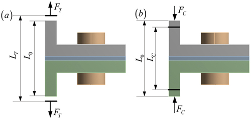
Based on the foregoing assumptions, the deformation of the bolt connection portion of the bolted flange joint shown in Figure 1(a) under axial tension is approximated by a combination of an elastic beam and two axial tension and compression springs, as shown in Figure 1(b), where Points B and C represent the touchpoints of bolts and flanges with gaskets.

Figure 1. Structure of a combination and an analogous model: (a) The fundamental bolted flange joint; and (b) The bolted flange joint’s corresponding axial double spring-bending beam model.

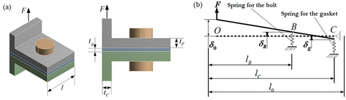
The balanced equation for the beam in the axial direction and the balanced equation for the bending moment at point C may be written as follows:

Under the action of axial tension, the balanced equation of the bending moment at point C can be expressed as:

(1) $F+F_g-F_B=0$(1)

(2) $F_B(l_C-l_B)-F\times l_C=0$(2)

Where $F$ denotes the axial tension load, $F_g$ is the axial pressure of the gasket at the point $C$, and $F_B$ is the bolt axial tension, $l_B$ is the mounting position of the bolt, and $l_C$ is the slot width of the flange.

When combined with the deformation of the top of the spring that simplified the bolt, the model’s displacement and deformation may be coordinated as follows.

(3) ${\delta }_B={\omega }_B-{\delta }_g$(3)

(4) ${\omega }_B=\frac{F{\left(l_C-l_B\right)}^2\left[3l_C-\left(l_C-l_B\right)\right]}{6E_{FL}{I}_{FL}}-\frac{F_B{\left(l_C-l_B\right)}^3}{3E_{FL}{I}_{FL}}$(4)

(5) ${\delta }_B=\frac{F{l}_C{t}_{FL}}{E_B{A}_B\left(l_C-l_B\right)}-\frac{F_{B0}{t}_{FL}}{E_B{A}_B}$(5)

(6) ${\delta }_g=\frac{F{l}_B{t}_g}{E_g{W}_f\left(l_O-l_C\right)\left(l_C-l_B\right)}$(6)

Where ${\omega }_B$ denotes the deflection deformation of the beam at the spring, ${\delta }_g$ denotes the axial deformation of the gasket, ${\delta }_B$ denotes the axial deformation of the spring, $E_{FL}$ is Young’s modulus of the flange material, and $E_B$ is Young’s modulus of the bolt material (the analytical model assumes that the gasket the material is linear elasticity), $t_g$ is the thickness of the gasket, $A_B$ is the area of the nominal diameter cross-section of the bolt, $W_f$ is the flange width, $I_{FL}$ is the moment of inertia of the flange section relative to the midplane, and $F_{BO}$ is the initial preload in the bolt.

By solving Equations(1)(1) $F+F_g-F_B=0$(1) , (2(2) $F_B(l_C-l_B)-F\times l_C=0$(2) ), and (4) simultaneously, all the unknown variables, $l_c$, $F_{\mathrm{g}}$ and $F_b$ are determined.

Due to the assumption of small linear elastic deformation, the axial deformation of the bolt connection part under tension (the transverse displacement of the beam’s free end) can be calculated by superimposing the external axial force and the bolt force-induced transverse deformation of the free end (Luan 2012).

(7) ${\delta }_0=\frac{F{l_c}^3}{3E_{FL}{I}_{FL}}-\frac{F_B{\left(l_c-l_B\right)}^2\left[3l_c-\left(l_c-l_B\right)\right]}{6E_{FL}{I}_{FL}}$(7)

When the flange is compressed, the axial deformation is mostly determined by the compression stiffness of the gasket and the flange in the axial direction (Alkatan et al. 2007). Therefore, the axial deformation of the connection section of the bolted flange joint may be described as

(8) ${\delta }_0=\frac{F\cdot \left(k_g+k_{FL}\right)}{k_g\cdot k_{FL}}$(8)

Where, $t_F$ denotes the thickness of the flange, and $t_C$ denotes the thickness of the connecting vertical plate, $k_g=E_g\cdot t_C\cdot l/t_s$ denotes the compression stiffness of the gasket, and $k_{FL}=E_{FL}\cdot t_C\cdot l/t_F$.

In summary, the bolt connection portion of the bolted flange joint’s axial nonlinear static displacement response may be described as

(9) ${\delta }_0=\left\{\begin{array}{c}\frac{F{l_c}^3}{3E_{FL}{I}_{FL}}-\frac{F_B{\left(l_c-l_B\right)}^2\left[3l_c-\left(l_c-l_B\right)\right]}{6E_{FL}{I}_{FL}},F>0\\ {\delta }_0=\frac{F\cdot \left(k_g+k_{FL}\right)}{k_g\cdot k_{FL}},\hspace{0.17em}F\le 0\end{array}\right.$(9)

3. Simulation calculation of fine finite element (FE) model

3.1. Gasket material property determination

Consider the influence on the axial stiffness of the bolted flange joint of aluminum alloy gaskets (linear elastic materials) and graphite gaskets (non-linear materials). The material parameters of the bolted flange joint’s components and a selection of aluminum alloy gaskets are listed in Table 1.

Table 1. Component’s material parameter.

Parts	Elastic ModulusE/GPa	Poisson’s ratio ν	Densityρ/(kg∙m^−3)
Bolt Flange Aluminum alloy gasket	210 210 71	0.31 0.31 0.33	7850 7850 2750

Compressive and elastomeric properties of graphite gaskets are highly dependent on the material and production circumstances and must be examined independently (Figure 2). At room temperature, the elasticity of the graphite gasket sample investigated in this research was determined using a Zwick-100kN static material testing equipment in line with GB/T 12622–2008 “Test Method for Compression and Resilience of Gaskets for Pipe Flanges” (Luan 2012). The gasket’s starting load is 1 MPa, the loading and unloading rate is 0.5MPa/s, the preload is 90MPa, and the specimen’s recorded compression resilience data are shown in Table 2.

Figure 2. Experiment on the compressive-resilient performance of cylinder gasket.

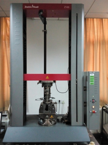
Table 2. Graphite gasket compression resilience test data.

Compression		Resilience
Strain	stress/MPa	Strain	stress/MPa
0.035	2.61	0.181	85.96
0.043	5.31	0.179	63.62
0.056	12.08	0.175	49.43
0.066	20.22	0.171	33.79
0.073	28.34	0.168	15.53
0.085	39.87	0.161	8.78
0.111	54.08	0.155	4.18
0.130	66.28	0.144	2.12
0.141	71.68	0.135	0.66

Fit the compression/resilience test data for the gasket to generate the compression and resilience curves for the gasket material under various loads (30MPa, 40MPa, 60MPa, 90MPa) (Figure 3).

Figure 3. Compressive-resilient performance curves of graphite gasket.

3.2. Finite element calculation and comparison calculation

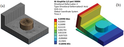
Taking into consideration the symmetry of the bolted flange joint structure and removing the top flange, bolts, and gaskets, as illustrated in Figure 4, to validate the construction of the fine finite element model by ANSYS. Coulomb friction contact is used to connect the model’s different components, and a pre-tightening unit is mounted on the bolt screw’s cylindrical surface to deliver the pre-tightening force.

Figure 4. Static finite element calculation of the bolted flange joint: (a) Basic bolted flange joint finite element model and (b) Overall axial deformation (FE).

The axial load-displacement curve of a composite construction made up of several gasket materials is shown in Figure 5. The axial stiffness is expressed as the slope of the curve. As seen in Figure 5, the bolted flange joint of gaskets made of various materials does not display the same nonlinear axial stiffness characteristics: (1) When a compressive load is applied, the stiffness of the axial load-displacement curve is greatly enhanced compared to when tension is applied; the combination structure of graphite shims exhibits less stiffness change when the axial load direction is changed. This is because the combined structure’s stress surface changes with the axial load direction, resulting in a change in contact stress, and because the linear elastic material shims in the combined structure are more sensitive to the stress change than the non-linear material shims. (2) When tension and compression loads are applied to the linear elastic material gasket, the axial stiffness of the structure remains constant. For the bolted flange joint of the non-linear graphite material gasket, the axial stiffness varies with load, indicating the bolted flange joint’s axial nonlinearity. Comparing the calculated value of the equivalent model by MATLAB to the value obtained from the fine finite element simulation reveals that the calculated value of the equivalent model is also in good agreement with the analytical result obtained from the precision model, error of less than 5%, and thus this equivalent model is used in the subsequent analysis of this article.

Figure 5. The load-displacement curve of the combination structure: (a) Non-linear materials and (b) Linear elastic material.

4. Linear and nonlinear simplification of spring stiffness and mass-spring system

As a result of the preceding discussion, it is clear that under certain conditions, the axial static load-displacement curve performance of the bolt flange structure is linear or nonlinear (as shown in Figure 6(a-d) are the load-displacement curves of primary, secondary, and tertiary, respectively). To model the dynamic properties of the bolted flange joint under this axial stiffness, uniaxial tension, and compression stiffness conditions, linear and nonlinear springs are presented in this section (Figure 7). Equations (11)(11) $k\left(\delta \right)=\left\{\begin{array}{c}a\\ 2a\delta +b\\ \left\{\begin{array}{c}a,\delta \ge 0\\ b,\delta <0\end{array}\right.\\ 3a{\delta }^2+2b\delta +c\end{array}\right.$(11) and (12(12) $\left\{\begin{array}{c}{k}_{+}=\frac{F_T}{L_T-L_0}\\ k_{-}=\frac{F_C}{L_0-L_C}\end{array}\right.$(12) ) approximate the connection between the axial load position and displacement, as well as the relationship between the axial stiffness and displacement, of the bolted flange joint composed of aluminum alloy and graphite gaskets.

Figure 6. Linear and nonlinear spring load-displacement curves.

Figure 7. Linear and nonlinear spring stiffness-displacement curves.

(10) $F\left(\delta \right)=\left\{\begin{array}{c}a\delta \\ a{\delta }^2+b\delta \\ \left\{\begin{array}{c}a\delta ,\delta \ge 0\\ b\delta ,\delta <0\end{array}\right.\\ a{\delta }^3+b{\delta }^2+c\delta \end{array}\right.$(10)

(11) $k\left(\delta \right)=\left\{\begin{array}{c}a\\ 2a\delta +b\\ \left\{\begin{array}{c}a,\delta \ge 0\\ b,\delta <0\end{array}\right.\\ 3a{\delta }^2+2b\delta +c\end{array}\right.$(11)

Where a, b, c, and d are all constants, which can be obtained by fitting the load-displacement curve; $F\left(\delta \right)$ is the axial load, $k\left(\delta \right)$ is the axial stiffness, and $\delta$ is the axial displacement.

Finite element analysis may be used to determine the tensile stiffness $k_{+}$ and compression stiffness $k_{-}$. To account for external deformation of the flange surface and an uneven distribution of the bolt connection part’s local displacement, the axial relative displacement is taken here as the value of the gap between the contact surfaces, rather than for the portion of the flange that is connected to the column section. Axial deformation is quantified (Figure 8). In other words, the nonlinear spring does not reflect bolts and washers but rather the complete bolt connection part’s axial stiffness characteristics (Luan 2012).

Figure 8. Deformation of the combination structure:(a) the axial tension state (b) the axial compression state.

Thus, for the bolt connection portion of the bolt flange gasket connection combination structure shown in Figure 8, the spring’s axial tension and compression stiffnesses may be represented as

(12) $\left\{\begin{array}{c}{k}_{+}=\frac{F_T}{L_T-L_0}\\ k_{-}=\frac{F_C}{L_0-L_C}\end{array}\right.$(12)

Where $F_T$ is the axial tension acting on the bolt connection part, where $F_C$ is the axial pressure acting on the bolt connection part, where $L_0$ is the axial length including the thickness of the flange and gasket, and where $L_T$ is the axial relative displacement of the bolt connection part under tension, and where $L_C$ is the axial relative displacement of the bolt connection part under pressure.

To investigate the dynamic response mechanism of the bolt-flange-gasket connection combination structure under non-linear tension and compression stiffness, only the top half of the bolt connection part is introduced, and the spring is put in the bolt connection part. The bolt connection is simplified, as seen in Figure 9. The spring indicates not only the contact stiffness but also the non-linear stiffness of the gasket material; in other words, the spring represents the stiffness of the bolted flange joint’s bolt connection.

Figure 9. Mass-spring system.

If the equilibrium position of the spring is used as the border of the motion zones (Equation (14)(14) $\mathbf{M}\ddot{\mathbf{y}}+\mathbf{K}\mathbf{y}=0$(14) ), the vibration of the mass-spring system in the $\left(u,\theta \right)$ plane may be separated into four zones as illustrated in Figure 10. By partitioning the system’s motion, each vibration area contains a unique combination of spring compression and tension states that is distinct from the other areas, and each partition is independent; on the other hand, the four regions completely cover the system’s motion plane, and any state of the system’s motion can be attributed to one of the four partitions, indicating that the region is completely partitioned (Luan 2012). As a result, the equations of motion for each vibration area may be solved independently of the spring’s state.

Figure 10. Division of the motion.

(13) $\left\{\begin{array}{c}{\delta }_1=u+L\theta =0\\ {\delta }_2=u-L\theta =0\end{array}\right.$(13)

5. Dynamic response mechanism of the mass-spring two-degree-of-freedom system under transverse load

Due to the linear or nonlinear axial stiffness of the spring in this model, under the action of transverse load, the center of mass may also create relative axial displacement while the mass produces a rotation angle. To investigate the dynamic response mechanism of the bolt-flange-gasket connection combination structure under transverse load with linear or nonlinear axial tension and compression stiffness, it is also assumed that both sides of the connection structure are symmetrical in the gasket center plane and that only the bolt connection is chosen. The top half of the component, together with the addition of springs, simplifies the bolt connection section into a two-degree-of-freedom mass-spring system (Figure 11). The mass’s out-of-plane deformation is not addressed here.

Figure 11. Deformation of a double-degree-of-freedom mass-spring system under transverse load.

The bolt flange gasket connection combination structure is abstracted as a mass-spring two-degree-of-freedom system using the preceding simplification. The system’s motion may be characterized by the displacements $\left({\delta }_1,{\delta }_2\right)$ of the two springs ${\delta }_1,{\delta }_2$ or by the axial and angular displacements of the center of mass $O$.

Currently, the system’s two-degree-of-freedom undamped free vibration control equation is

(14) $\mathbf{M}\ddot{\mathbf{y}}+\mathbf{K}\mathbf{y}=0$(14)

Where $y={\left(u,\theta \right)}^T$ is the displacement vector; $M=\left[\begin{array}{c}m0\\ 0J\end{array}\right]$ is the system mass matrix; $K$ is the system stiffness matrix.

The kinetic energy of the system can be expressed as

(15) $T=\frac{1}{2}m{\dot{u}}^2+\frac{1}{2}J{\dot{\theta }}^2$(15)

The elastic potential energy of the system can be expressed as

(16) $U=\frac{1}{2}\left(k_1{\delta }_1^2+k_2{\delta }_2^2\right)$(16)

The conversion relationship between the displacement of the O point and the spring deformation ${\delta }_1,{\delta }_2$ as follows.

(17) $\left(\begin{array}{c}{\delta }_1\\ {\delta }_2\end{array}\right)=\left[\begin{array}{c}1L\\ 1-L\end{array}\right]\left(\begin{array}{c}u\\ \theta \end{array}\right)$(17)

Where L denotes the radius width of the bolted flange joint, i.e. the distance between the opposing springs and the bolted flange joint’s central axis.

As a result of the spring stiffness simplification, the free vibration control equations for the mass-spring two-degree-of-freedom system are solved individually.

5.1. Same stiffness spring (linear simplified model, that is, the spring stiffness is constant $k_1=k_2=k_{\mathrm{\_}}=k_{+}=a_{\left.\hspace{0.17em}\right)}$)

By taking the generalized coordinates as $\left(u,\theta \right)$, translating the system’s kinetic energy and elastic potential energy into variables $\left(u,\theta \right)$, and inserting them into the Lagrange equation, one may derive the system’s undamped free vibration equation:

(18) $\left[\begin{array}{c}m\\ 0\end{array}\right.\left.\begin{array}{c}0\\ J\end{array}\right]\left(\begin{array}{c}\ddot{u}\\ \ddot{\theta }\end{array}\right)+\left[\begin{array}{c}2a\\ 0\end{array}\right.\left.\begin{array}{c}0\\ 2a{L}^2\end{array}\right]\left(\begin{array}{c}u\\ \theta \end{array}\right)=0$(18)

The motion equation may be solved for the given starting circumstances just by finding the coefficient of the first-order component in the load-displacement curve, and it can be shown that the transverse vibration response of the system is connected to the geometric structure L of the system.

The mass matrix and stiffness matrix of the system are both diagonals, as shown by the control equation. At this point, the vertical vibration of the system and the rotation around the center of mass are independent.

5.2. Tension and compression stiffness nonlinear spring (non-linear simplified model, namely $k=2a\delta +b$)

Taking the generalized coordinates as $\left({\delta }_1,{\delta }_2\right)$, then $u$ and $\theta$ can be expressed as follows:

(19) $\left(\begin{array}{c}u\\ \theta \end{array}\right)=\left[\begin{array}{c}1/21/2\\ 1/2L-1/2L\end{array}\right]\left(\begin{array}{c}{\delta }_1\\ {\delta }_2\end{array}\right)$(19)

The stiffness of the spring may be represented as:

(20) $\left\{\begin{array}{c}{k}_1=2a{\delta }_1+b\\ k_2=2a{\delta }_2+b\end{array}\right.$(20)

By substituting the particle’s kinetic energy and elastic potential energy in generalized coordinates ${\delta }_1$ and ${\delta }_2$ into the Lagrange equation, the two-degree-of-freedom system’s nonlinear undamped free vibration equation may be derived as:

(21) $\left[\begin{array}{c}\frac{m}{4}+\frac{J}{4L^2}\\ \frac{m}{4}-\frac{J}{4L^2}\end{array}\right.\left.\begin{array}{c}\frac{m}{4}-\frac{J}{4L^2}\\ \frac{m}{4}+\frac{J}{4L^2}\end{array}\right]\left(\begin{array}{c}{\ddot{\delta }}_1\\ {\ddot{\delta }}_2\end{array}\right)+\left[\begin{array}{c}3a\\ 0\end{array}\right.\left.\begin{array}{c}0\\ 3a\end{array}\right]{\left(\begin{array}{c}{\delta }_1\\ {\delta }_2\end{array}\right)}^2+\left[\begin{array}{c}b\\ 0\end{array}\right.\left.\begin{array}{c}0\\ b\end{array}\right]\left(\begin{array}{c}{\delta }_1\\ {\delta }_2\end{array}\right)=0$(21)

Where a, b, m, J, and L are all constants. Under the stated beginning circumstances, the equation of motion may be solved numerically. As can be seen from this calculation, the system’s reaction is entirely dependent on the geometric structure.

5.3. Tension and compression springs with different stiffness (bilinear simplified model $k=\left\{\begin{array}{c}a,\delta >0\\ b,\delta <0\end{array}\right.$)

By substituting the system’s kinetic and elastic potential energies into the Lagrange equation, one may derive the undamped free vibration control equation for the two-degree-of-freedom system in generalized coordinates $\left(u,\theta \right)$.

(22) $\left[\begin{array}{c}m\\ 0\end{array}\right.\left.\begin{array}{c}0\\ J\end{array}\right]\left(\begin{array}{c}\ddot{u}\\ \ddot{\theta }\end{array}\right)+\left[\begin{array}{c}{k}_1^{\ast }+k_2^{\ast }\\ L\left(k_1^{\ast }-k_2^{\ast }\right)\end{array}\right.\left.\begin{array}{c}L\left(k_1^{\ast }-k_2^{\ast }\right)\\ L^2\left(k_1^{\ast }+k_2^{\ast }\right)\end{array}\right]\left(\begin{array}{c}u\\ \theta \end{array}\right)=0$(22)

Where $k_1^{\ast }$ and $k_2^{\ast }$ denote the stiffness of springs 1 and 2, respectively. The precise value relies on the system’s motion state in the $\left(u,\theta \right)$ plane. Only the stiffness matrix, namely $k_1^{\ast }$ and $k_2^{\ast }$, is found, and the equation of motion for the given beginning circumstances may be calculated. To solve the challenge, its value must be equal to the bilinear stiffness of a system with one degree of freedom. Each area’s stiffness matrix should be established under the region of system motion. Simultaneously, the stiffness matrix is asymmetric owing to $k_1^{\ast }\ne k_2^{\ast }$, and the equations are elastically linked. Equation (23)(23) $\left\{\begin{array}{c}{k}_1=3a{{\delta }_1}^2+2b{\delta }_1+c\\ k_2=3a{{\delta }_2}^2+2b{\delta }_2+c\end{array}\right.$(23) demonstrates that the system’s reaction is entirely dependent on the geometric structure L.

5.4. Tension and compression stiffness nonlinear spring (non-linear simplified model, namely $k=3a{x}^2+2bx+c$)

The spring’s stiffness may be represented as

(23) $\left\{\begin{array}{c}{k}_1=3a{{\delta }_1}^2+2b{\delta }_1+c\\ k_2=3a{{\delta }_2}^2+2b{\delta }_2+c\end{array}\right.$(23)

In generalized coordinates $\left({\delta }_1,{\delta }_2\right)$, the undamped free vibration equation of the system may be found by putting the kinetic energy and elastic potential energy of the system into the Lagrange equation.

(24) $\left[{ }_{\frac{m}{4}+\frac{J}{4L^2}}^{{ }^{\frac{m}{4}+\frac{J}{4L^2}}}{}_{\frac{m}{4}+\frac{J}{4L^2}}^{\frac{m}{4}+\frac{J}{4L^2}}\right]\left({ }_{{\ddot{\delta }}_2}^{{\ddot{\delta }}_1}\right)+\left[{ }_0^{6a}{}_{6a}^0\right]{\left({ }_{{\delta }_2}^{{\delta }_1}\right)}^3+\left[{ }_0^{3b}{}_{3b}^0\right]{\left({ }_{{\delta }_2}^{{\delta }_1}\right)}^2+\left[{ }_0^c{}_c^0\right]\left({ }_{{\delta }_2}^{{\delta }_1}\right)=0$(24)

Where a, b, c, m, J, and L are all constants. Under the stated beginning circumstances, the equation of motion may be solved. As can be seen from this calculation, the system’s reaction is entirely dependent on the geometric structure L.

6. The solution of two-degree-of-freedom nonlinear dynamic response mechanism model under transverse load

6.1. Solve for linear spring with same stiffness (spring stiffness is constant)

Assume the controlling equation’s solution form is

(25) $\mathbf{y}=A{e}^{\left(\omega t+\varphi \right)i}$(25)

Where A denotes the amplitude; $\omega$ is the frequency of the natural vibration circle within the zone; $\varphi$ is the phase angle.

According to Equation (19)(19) $\left(\begin{array}{c}u\\ \theta \end{array}\right)=\left[\begin{array}{c}1/21/2\\ 1/2L-1/2L\end{array}\right]\left(\begin{array}{c}{\delta }_1\\ {\delta }_2\end{array}\right)$(19) , the system’s stiffness and mass matrices are diagonal matrices, and the matrix elements are calculated without coupling terms; at this point, the system’s vibration characteristic equation ($\left|K-{\omega }^{2}M\right|=0$) is defined.

(26) $\left|\left[\begin{array}{c}2a0\\ 02a{L}^2\end{array}\right]-{\omega }^2\left[\begin{array}{c}m\\ 0\end{array}\right.\left.\begin{array}{c}0\\ J\end{array}\right]\right|=0$(26)

Where $\omega$ denotes the vibration frequency of the system.

When the spring’s tension and compression stiffness are linear in the $\left(u,\theta \right)$ plane, the system’s transverse and axial vibration responses are independent. When the spring tension and compression stiffness are equal, the two-degree-of-freedom system’s axial vibration frequency is ${\omega }_1=\sqrt{2a/m}$ and the transverse vibration frequency is ${\omega }_2=\sqrt{2a{L}^2/J}$. The formations that correspond to ${\omega }_1$ and ${\omega }_2$ are ${\varphi }_1=\left(\begin{array}{c}1\\ 0\end{array}\right),{\varphi }_2=\left(\begin{array}{c}0\\ 1\end{array}\right)$ respectively.

The generic solution to the Equation (19)(19) $\left(\begin{array}{c}u\\ \theta \end{array}\right)=\left[\begin{array}{c}1/21/2\\ 1/2L-1/2L\end{array}\right]\left(\begin{array}{c}{\delta }_1\\ {\delta }_2\end{array}\right)$(19) is as follows:

(27) $\left\{\begin{array}{c}u\left(t\right)=C_{u1}cos{\omega }_{1}t+C_{u2}sin{\omega }_{1}t\\ \theta \left(t\right)=C_{\theta 1}cos{\omega }_{1}t+C_{\theta 2}sin{\omega }_{1}t\end{array}\right.$(27)

Where, $C_{u1}$,$C_{u2}$, $C_{\theta 1}$, and $C_{\theta 2}$ are undetermined coefficients.

Given initial conditions

(28) $\left\{\begin{array}{c}u\left(0\right)=u_0,\dot{u}\left(0\right)={\dot{u}}_0\\ \theta \left(0\right)={\theta }_0,\dot{\theta }\left(0\right)={\dot{\theta }}_0\end{array}\right.$(28)

All unknown coefficients may be derived by substituting Equation (28)(28) $\left\{\begin{array}{c}u\left(0\right)=u_0,\dot{u}\left(0\right)={\dot{u}}_0\\ \theta \left(0\right)={\theta }_0,\dot{\theta }\left(0\right)={\dot{\theta }}_0\end{array}\right.$(28) into Equation (29)(29) $\left\{\begin{array}{c}u\left(t\right)=u_{0}cos{\omega }_{1}t+\frac{{\dot{u}}_0}{{\omega }_1}sin{\omega }_{1}t\\ \theta \left(t\right)={\theta }_{0}cos{\omega }_{2}t+\frac{{\dot{\theta }}_0}{{\omega }_2}sin{\omega }_{2}t\end{array}\right.$(29) .

Thus, with the provided transversal beginning conditions, the system’s solution is obtained.

(29) $\left\{\begin{array}{c}u\left(t\right)=u_{0}cos{\omega }_{1}t+\frac{{\dot{u}}_0}{{\omega }_1}sin{\omega }_{1}t\\ \theta \left(t\right)={\theta }_{0}cos{\omega }_{2}t+\frac{{\dot{\theta }}_0}{{\omega }_2}sin{\omega }_{2}t\end{array}\right.$(29)

Observing the solution of the governing equation, $u\left(t\right)$ and $\theta \left(t\right)$ in Equation (30)(30) $\left[\begin{array}{c}\frac{m}{4}+\frac{J}{4L^2}\\ 0\end{array}\begin{array}{c}0\\ \frac{m}{4}+\frac{J}{4L^2}\end{array}\right]\left(\begin{array}{c}{\ddot{\delta }}_1\\ {\ddot{\delta }}_2\end{array}\right)+\left[\begin{array}{c}3a\\ 0\end{array}\begin{array}{c}0\\ 3a\end{array}\right]{\left(\begin{array}{c}{\delta }_1\\ {\delta }_2\end{array}\right)}^2+\left[\begin{array}{c}b\\ 0\end{array}\begin{array}{c}0\\ b\end{array}\right]\left(\begin{array}{c}{\delta }_1\\ {\delta }_2\end{array}\right)=0$(30) are fully independent; this indicates that the system’s initial angular velocity can only result in transverse rotation vibration.

6.2. Solving nonlinear spring with tension and compression stiffness (spring stiffness is a linear function of displacement)

Observing Equation (22)(22) $\left[\begin{array}{c}m\\ 0\end{array}\right.\left.\begin{array}{c}0\\ J\end{array}\right]\left(\begin{array}{c}\ddot{u}\\ \ddot{\theta }\end{array}\right)+\left[\begin{array}{c}{k}_1^{\ast }+k_2^{\ast }\\ L\left(k_1^{\ast }-k_2^{\ast }\right)\end{array}\right.\left.\begin{array}{c}L\left(k_1^{\ast }-k_2^{\ast }\right)\\ L^2\left(k_1^{\ast }+k_2^{\ast }\right)\end{array}\right]\left(\begin{array}{c}u\\ \theta \end{array}\right)=0$(22) , the mass matrix of the system in generalized coordinates ${\delta }_1$ and ${\delta }_2$ is symmetric, the elements are determined, and the stiffness matrix of the system is diagonal; moreover, when $\frac{m}{4}-\frac{J}{4L^2}=0$, that is when $m{L}^2=J$, the mass matrix is diagonal and the equations are decoupled. When $\frac{m}{4}-\frac{J}{4L^2}\ne 0$ the mass matrix, specifically $m{L}^2\ne J$, is symmetric, the equations exhibit inertial coupling.

When the equations are decoupled, the vibration’s generalized coordinates ${\delta }_1$ and ${\delta }_2$ are independent of one another, and the system’s nonlinear vibration control equation is

(30) $\left[\begin{array}{c}\frac{m}{4}+\frac{J}{4L^2}\\ 0\end{array}\begin{array}{c}0\\ \frac{m}{4}+\frac{J}{4L^2}\end{array}\right]\left(\begin{array}{c}{\ddot{\delta }}_1\\ {\ddot{\delta }}_2\end{array}\right)+\left[\begin{array}{c}3a\\ 0\end{array}\begin{array}{c}0\\ 3a\end{array}\right]{\left(\begin{array}{c}{\delta }_1\\ {\delta }_2\end{array}\right)}^2+\left[\begin{array}{c}b\\ 0\end{array}\begin{array}{c}0\\ b\end{array}\right]\left(\begin{array}{c}{\delta }_1\\ {\delta }_2\end{array}\right)=0$(30)

The time historical response of the system in generalized coordinates ${\delta }_1$ and ${\delta }_2$ may be derived by using the ODE solver in MATLAB to conduct numerical integration operations on the vibration control equations. By including the responses of ${\delta }_1$ and ${\delta }_2$ into Equation (20)(20) $\left\{\begin{array}{c}{k}_1=2a{\delta }_1+b\\ k_2=2a{\delta }_2+b\end{array}\right.$(20) , one may derive the system’s vibration response in the $\left(u,\theta \right)$ plane using matrix operation.

When the equations are unable to be decoupled, the vibrations of the generalized coordinates ${\delta }_1$ and ${\delta }_2$ become connected. At the moment, the system’s governing equation is as follows:

(31) $\left[\begin{array}{c}\frac{m}{4}+\frac{J}{4L^2}\\ \frac{m}{4}-\frac{J}{4L^2}\end{array}\begin{array}{c}\frac{m}{4}-\frac{J}{4L^2}\\ \frac{m}{4}+\frac{J}{4L^2}\end{array}\right]\left(\begin{array}{c}{\ddot{\delta }}_1\\ {\ddot{\delta }}_2\end{array}\right)+\left[\begin{array}{c}3a\\ 0\end{array}\begin{array}{c}0\\ 3a\end{array}\right]{\left(\begin{array}{c}{\delta }_1\\ {\delta }_2\end{array}\right)}^2+\left[\begin{array}{c}b\\ 0\end{array}\begin{array}{c}0\\ b\end{array}\right]\left(\begin{array}{c}{\delta }_1\\ {\delta }_2\end{array}\right)=0$(31)

Due to the nonlinear nature of the vibration equation, the complete control equation cannot be decoupled by coordinate changes. As a result, the control equation exhibits inertial but not elastic coupling. If the second-order coefficient matrix determinant is not equal to zero, i.e., the system mass matrix determinant is not equal to zero, then there exists an inverse matrix of the second-order coefficient matrix, and for each term in equation (42)(42) $C_1=\frac{{\theta }_0-r_2{u}_0}{r_1-r_2},C_2=\frac{{\dot{\theta }}_0-r_2{\dot{u}}_0}{{\omega }_1\left(r_1-r_2\right)},C_3=\frac{u_0-r_2{\theta }_0}{r_1-r_2},\text{break}{C}_4=\frac{{\dot{u}}_0-r_2{\dot{\theta }}_0}{{\omega }_2\left(r_1-r_2\right)}$(42) left multiplied by the inverse matrix of the second-order coefficient matrix, the equation’s second-order derivative terms are decoupled. At this point, given a starting value for the nonlinear equation, the ODE solver in MATLAB can be used to conduct numerical integration to get the numerical solution of the vibration equation, as well as the time history response of the generalized coordinates ${\delta }_1$ and ${\delta }_2$. By including the responses of ${\delta }_1$ and ${\delta }_2$ into Equation (20)(20) $\left\{\begin{array}{c}{k}_1=2a{\delta }_1+b\\ k_2=2a{\delta }_2+b\end{array}\right.$(20) , one may derive the system’s vibration response in the $\left(u,\theta \right)$ plane using matrix operation.

6.3. Solution of tension and compression bilinear stiffness spring (bilinear simplified model)

According to Equation (23)(23) $\left\{\begin{array}{c}{k}_1=3a{{\delta }_1}^2+2b{\delta }_1+c\\ k_2=3a{{\delta }_2}^2+2b{\delta }_2+c\end{array}\right.$(23) , the mass matrix of the system in the $\left(u,\theta \right)$ plane is diagonal, and each element of the matrix is determined independently of the coupling items; however, the stiffness matrix of the system is dependent on the system’s vibration state under transverse load, specifically the spring tension and compression state. When the spring tension and compression stiffness are bilinear, the system has four motion states in the $\left(u,\theta \right)$ plane. Each of these four motion states corresponds to a deterministic system of equations that can be solved analytically using the method for solving linear equations. Luan (2012) created the system’s vibration control equation for bilinear spring tension and compression stiffness. This article discusses the control equation he developed. The distinction is that the spring displacement is used to determine the solution of the control equation.

The stiffness matrix for each location is computed according to the spring’s tension and compression condition during movement (Table 3), and then the motion equations for each zone are solved independently.

Table 3. Spring state and stiffness matrix of each vibration area (Luan 2012).

Area	(${\delta }_1,{\delta }_2$)	($u,\theta$)	${k_1}^{\ast },{k_2}^{\ast }$	Stiffness matrix K
I	$\begin{array}{rl}& {\delta }_1\ge 0\\ & {\delta }_2\ge 0\end{array}$	$\begin{array}{rl}& u>0\\ & -\frac{1}{L}u<\theta <\frac{1}{L}u\end{array}$	$\begin{array}{rl}& {k_1}^{\ast }=k_{+}\\ & {k_2}^{\ast }=k_{+}\end{array}$	$\left[\begin{array}{c}2k_{+}0\\ 02L^2{k}_{+}\end{array}\right]$
II	$\begin{array}{rl}& {\delta }_1<0\\ & {\delta }_2>0\end{array}$	$\begin{array}{rl}& -\frac{1}{L}\theta <u<\frac{1}{L}\theta \\ & \theta >0\end{array}$	$\begin{array}{rl}& k_1\ast =k_{+}\\ & k_2\ast =k_{\mathrm{\_}}\end{array}$	$\left[\begin{array}{c}{k}_{+}+k_{-}L\left(k_{+}-k_{-}\right)\\ L\left(k_{+}-k_{-}\right)L^2\left(k_{+}+k_{-}\right)\end{array}\right]$
III	$\begin{array}{rl}& {\delta }_1<0\\ & {\delta }_2<0\end{array}$	$\begin{array}{rl}& u<0\\ & \frac{1}{L}u<\theta <-\frac{1}{L}u\end{array}$	$\begin{array}{rl}& k_1\ast =k_{-}\\ & k_2\ast =k_{\mathrm{\_}}\end{array}$	$\left[\begin{array}{c}2k_{-}0\\ 02L^2{k}_{-}\end{array}\right]$
IV	$\begin{array}{rl}& {\delta }_1>0\\ & {\delta }_2<0\end{array}$	$\begin{array}{rl}& \frac{1}{L}\theta <u<-\frac{1}{L}\theta \\ & \theta <0\end{array}$	$\begin{array}{rl}& {k_1}^{\ast }=k_{-}\\ & {k_2}^{\ast }=k_{+}\end{array}$	$\left[\begin{array}{c}{k}_{+}+k_{-}L\left(k_{-}-k_{+}\right)\\ L\left(k_{-}-k_{+}\right)L^2\left(k_{+}+k_{-}\right)\end{array}\right]$

When a transverse force acts, and the load-displacement curve is bilinear, the system vibrates throughout the full $\left(u,\theta \right)$ plane of motion. Assume that the solution to the system’s control equation in these four divisions has the form of

(32) $\mathbf{y}=A{e}^{\left(\omega t+\varphi \right)i}$(32)

Where A is the amplitude; $\omega$ is the frequency of the natural vibration circle within the zone; $\varphi$ is the phase angle.

1. Area I (${\delta }_1\ge 0,{\delta }_2\ge 0$)

For area I, the system’s two springs are both under tension, and the stiffnesses are both taken as $k_{+}$; according to Table 2, the system’s motion equation in area I is

(33) $\left[\begin{array}{c}m\\ 0\end{array}\right.\left.\begin{array}{c}0\\ J\end{array}\right]\left(\begin{array}{c}\ddot{u}\\ \ddot{\theta }\end{array}\right)+\left[\begin{array}{c}2k_{+}0\\ 02L^2{k}_{+}\end{array}\right]\left(\begin{array}{c}u\\ \theta \end{array}\right)=0$(33)

By examining the Equation (34)(34) $\left|\left[\begin{array}{c}2k_{+}0\\ 02L^2{k}_{+}\end{array}\right]-{\omega }^2\left[\begin{array}{c}m\\ 0\end{array}\right.\left.\begin{array}{c}0\\ J\end{array}\right]\right|=0$(34) , it is clear that the system’s axial vibration has no connection to L, but the transverse vibration has a strong link to L. In this situation, the system’s vibration characteristic equation ($\left|K-{\omega }^{2}M\right|=0$) is

(34) $\left|\left[\begin{array}{c}2k_{+}0\\ 02L^2{k}_{+}\end{array}\right]-{\omega }^2\left[\begin{array}{c}m\\ 0\end{array}\right.\left.\begin{array}{c}0\\ J\end{array}\right]\right|=0$(34)

Where $\omega$ denotes the system’s vibration frequency. The vibration control equation (Equation (34)(34) $\left|\left[\begin{array}{c}2k_{+}0\\ 02L^2{k}_{+}\end{array}\right]-{\omega }^2\left[\begin{array}{c}m\\ 0\end{array}\right.\left.\begin{array}{c}0\\ J\end{array}\right]\right|=0$(34) demonstrates that the system’s axial vibration response under transverse load is independent of its transverse vibration response. For the area I, the system’s axial vibration frequency is ${\omega }_1=\sqrt{2k_{+}/m}$, its transverse vibration frequency is ${\omega }_2=\sqrt{2L^2{k}_{+}/J}$, the corresponding formations of ${\omega }_1$ and ${\omega }_2$ are ${\varphi }_1=\left(\begin{array}{c}1\\ 0\end{array}\right),{\varphi }_2=\left(\begin{array}{c}0\\ 1\end{array}\right)$, and the system’s general solution may be expressed as:

(35) $\left\{\begin{array}{c}u\left(t\right)=C_{u1}cos{\omega }_{1}t+C_{u2}sin{\omega }_{1}t\\ \theta \left(t\right)=C_{\theta 1}cos{\omega }_{1}t+C_{\theta 2}sin{\omega }_{1}t\end{array}\right.$(35)

Where $C_{u1}$,$C_{u2}$, $C_{\theta 1}$, and $C_{\theta 2}$ are undetermined coefficients.

Given initial conditions

(36) $\left\{\begin{array}{c}u\left(0\right)=u_0,\dot{u}\left(0\right)={\dot{u}}_0\\ \theta \left(0\right)={\theta }_0,\dot{\theta }\left(0\right)={\dot{\theta }}_0\end{array}\right.$(36)

By putting Equation (37)(37) $\left\{\begin{array}{c}u\left(t\right)=u_{0}cos{\omega }_{1}t+\frac{{\dot{u}}_0}{{\omega }_1}sin{\omega }_{1}t\\ \theta \left(t\right)={\theta }_{0}cos{\omega }_{2}t+\frac{{\dot{\theta }}_0}{{\omega }_2}sin{\omega }_{2}t\end{array}\right.$(37) into Equation (36)(36) $\left\{\begin{array}{c}u\left(0\right)=u_0,\dot{u}\left(0\right)={\dot{u}}_0\\ \theta \left(0\right)={\theta }_0,\dot{\theta }\left(0\right)={\dot{\theta }}_0\end{array}\right.$(36) , all undetermined coefficients may be determined.

Thus, given the initial transverse circumstances, the system in area I has a solution:

(37) $\left\{\begin{array}{c}u\left(t\right)=u_{0}cos{\omega }_{1}t+\frac{{\dot{u}}_0}{{\omega }_1}sin{\omega }_{1}t\\ \theta \left(t\right)={\theta }_{0}cos{\omega }_{2}t+\frac{{\dot{\theta }}_0}{{\omega }_2}sin{\omega }_{2}t\end{array}\right.$(37)

As seen in Equation (38)(38) $\left[\begin{array}{c}m\\ 0\end{array}\right.\left.\begin{array}{c}0\\ J\end{array}\right]\left(\begin{array}{c}\ddot{u}\\ \ddot{\theta }\end{array}\right)+\left[\begin{array}{c}{k}_{+}+k_{-}\\ L\left(k_{+}-k_{-}\right)\end{array}\right.\left.\begin{array}{c}L\left(k_{+}-k_{-}\right)\\ L^2\left(k_{+}+k_{-}\right)\end{array}\right]\left(\begin{array}{c}u\\ \theta \end{array}\right)=0$(38) $u\left(t\right)$ and $\theta \left(t\right)$ are independent, the initial transverse rotation speed can only induce rotational vibration.

• (2) Area II (${\delta }_1⟨0,{\delta }_2⟩0$)

For area II, the system’s vibration motion is divided into tension and compression. The right spring 1 is in tension while the left spring 2 is in compression. At this point, the two-degree-of-freedom system’s motion control equation is

(38) $\left[\begin{array}{c}m\\ 0\end{array}\right.\left.\begin{array}{c}0\\ J\end{array}\right]\left(\begin{array}{c}\ddot{u}\\ \ddot{\theta }\end{array}\right)+\left[\begin{array}{c}{k}_{+}+k_{-}\\ L\left(k_{+}-k_{-}\right)\end{array}\right.\left.\begin{array}{c}L\left(k_{+}-k_{-}\right)\\ L^2\left(k_{+}+k_{-}\right)\end{array}\right]\left(\begin{array}{c}u\\ \theta \end{array}\right)=0$(38)

By examining the Equation (39)(39) $\left|\left[\begin{array}{c}{k}_{+}+k_{-}\\ L\left(k_{+}-k_{-}\right)\end{array}\right.\left.\begin{array}{c}L\left(k_{+}-k_{-}\right)\\ L^2\left(k_{+}+k_{-}\right)\end{array}\right]-{\omega }^2\left[\begin{array}{c}m\\ 0\end{array}\right.\left.\begin{array}{c}0\\ J\end{array}\right]\right|=0$(39) , it is clear that the system’s axial and transverse vibrations are highly connected to L, and that the system’s vibration characteristic equation ($\left|K-{\omega }^{2}M\right|=0$) is

(39) $\left|\left[\begin{array}{c}{k}_{+}+k_{-}\\ L\left(k_{+}-k_{-}\right)\end{array}\right.\left.\begin{array}{c}L\left(k_{+}-k_{-}\right)\\ L^2\left(k_{+}+k_{-}\right)\end{array}\right]-{\omega }^2\left[\begin{array}{c}m\\ 0\end{array}\right.\left.\begin{array}{c}0\\ J\end{array}\right]\right|=0$(39)

Solving the Equation (40)(40) $\left\{\begin{array}{c}{\omega }_1^2=\frac{m{k}_3+J{k}_1-\sqrt{{\left(m{k}_3-J{k}_1\right)}^2+4mJ{k}_2^2}}{2mJ}\\ {\omega }_2^2=\frac{m{k}_3+J{k}_1+\sqrt{{\left(m{k}_3-J{k}_1\right)}^2+4mJ{k}_2^2}}{2mJ}\end{array}\right.$(40) , the natural frequency of the system in area II is

(40) $\left\{\begin{array}{c}{\omega }_1^2=\frac{m{k}_3+J{k}_1-\sqrt{{\left(m{k}_3-J{k}_1\right)}^2+4mJ{k}_2^2}}{2mJ}\\ {\omega }_2^2=\frac{m{k}_3+J{k}_1+\sqrt{{\left(m{k}_3-J{k}_1\right)}^2+4mJ{k}_2^2}}{2mJ}\end{array}\right.$(40)

Due to the presence of non-diagonal components in the stiffness matrix at this point, the solutions to and cannot be entirely decoupled; the forms (eigenvalues) of the equations of motion corresponding to ${\omega }_1^2$ and ${\omega }_2^2$ are ${\varphi }_1=\left(\begin{array}{c}1\\ r_1\end{array}\right),{\varphi }_2=\left(\begin{array}{c}1\\ r_2\end{array}\right)$ respectively, where $r_1=\frac{k_1-m{\omega }_1^2}{k_2}=\frac{k_2}{k_3-J{\omega }_1^2},r_2=\frac{k_1-m{\omega }_2^2}{k_2}=\frac{k_2}{k_3-J{\omega }_2^2}$.

Thus, the general solution of motion may be written as:

(41) $\left\{\begin{array}{c}u\left(t\right)=C_{1}cos{\omega }_{1}t+C_{2}sin{\omega }_{1}t+C_{3}cos{\omega }_{2}t+C_{4}sin{\omega }_{2}t\\ \theta \left(t\right)=r_1\left(C_{1}cos{\omega }_{1}t+C_{2}sin{\omega }_{1}t\right)+r_2\left(C_{3}cos{\omega }_{2}t\text{break}+C_{4}sin{\omega }_{2}t\right)\end{array}\right.$(41)

Where $C_1$,$C_2$,$C_3$ and $C_4$ are undetermined coefficients.

All coefficients in the general solution may be obtained by inserting Equation (42)(42) $C_1=\frac{{\theta }_0-r_2{u}_0}{r_1-r_2},C_2=\frac{{\dot{\theta }}_0-r_2{\dot{u}}_0}{{\omega }_1\left(r_1-r_2\right)},C_3=\frac{u_0-r_2{\theta }_0}{r_1-r_2},\text{break}{C}_4=\frac{{\dot{u}}_0-r_2{\dot{\theta }}_0}{{\omega }_2\left(r_1-r_2\right)}$(42) into the starting condition (Equation (37)(37) $\left\{\begin{array}{c}u\left(t\right)=u_{0}cos{\omega }_{1}t+\frac{{\dot{u}}_0}{{\omega }_1}sin{\omega }_{1}t\\ \theta \left(t\right)={\theta }_{0}cos{\omega }_{2}t+\frac{{\dot{\theta }}_0}{{\omega }_2}sin{\omega }_{2}t\end{array}\right.$(37) ):

(42) $C_1=\frac{{\theta }_0-r_2{u}_0}{r_1-r_2},C_2=\frac{{\dot{\theta }}_0-r_2{\dot{u}}_0}{{\omega }_1\left(r_1-r_2\right)},C_3=\frac{u_0-r_2{\theta }_0}{r_1-r_2},\text{break}{C}_4=\frac{{\dot{u}}_0-r_2{\dot{\theta }}_0}{{\omega }_2\left(r_1-r_2\right)}$(42)

By examining the analytical solution to the motion control equation in area II, it is possible to determine that the axial and transverse vibration responses of the two-degree-of-freedom system are coupled vibrations: that is, the initial axial velocity will inevitably cause transverse rotation vibration; otherwise, the initial transverse rotation velocity will inevitably cause axial vibration. This is because the stiffness matrix of the vibration control equation has an elastic coupling factor; the underlying reason for the elastic coupling term is that the system’s axial tension and compression stiffness are nonlinear.

• (3) Area III (${\delta }_1<0,{\delta }_2<0$)

For area III, the system’s two springs are compressed, and their stiffness is denoted by $k_{-}$; at this point, the system’s motion regulating equation is

(43) $\left[\begin{array}{c}m\\ 0\end{array}\right.\left.\begin{array}{c}0\\ J\end{array}\right]\left(\begin{array}{c}\ddot{u}\\ \ddot{\theta }\end{array}\right)+\left[\begin{array}{c}2k_{-}0\\ 02L^2{k}_{-}\end{array}\right]\left(\begin{array}{c}u\\ \theta \end{array}\right)=0$(43)

The motion equation of zone III is approximately the same as the vibration equation of zone I. Due to the absence of elastic coupling factors in the stiffness matrix of the vibration regulating equation, the transverse and axial vibration responses of the system under transverse load are independent. The frequency and mode shape of area III are:

(44) ${\omega }_1^2=\frac{2k_{-}}{m},{\omega }_2^2=\frac{2L^2{k}_{-}}{J}$(44)

(45) ${\varphi }_1=\left(\begin{array}{c}1\\ 0\end{array}\right),{\varphi }_2=\left(\begin{array}{c}0\\ 1\end{array}\right)$(45)

Where ${\omega }_1$ and ${\varphi }_1$ denote the frequency and mode shape of the axial vibration, respectively; ${\omega }_2$ and ${\varphi }_2$ denote the frequency and mode shape of the rotational vibration, respectively.

As with vibration area I, the general solution of area III for the starting state (equation (37)(37) $\left\{\begin{array}{c}u\left(t\right)=u_{0}cos{\omega }_{1}t+\frac{{\dot{u}}_0}{{\omega }_1}sin{\omega }_{1}t\\ \theta \left(t\right)={\theta }_{0}cos{\omega }_{2}t+\frac{{\dot{\theta }}_0}{{\omega }_2}sin{\omega }_{2}t\end{array}\right.$(37) ) is derived as

(46) $\left\{\begin{array}{c}u\left(t\right)=u_{0}cos{\omega }_{1}t+\frac{{\dot{u}}_0}{{\omega }_1}sin{\omega }_{1}t\\ \theta \left(t\right)={\theta }_{0}cos{\omega }_{2}t+\frac{{\dot{\theta }}_0}{{\omega }_2}sin{\omega }_{2}t\end{array}\right.$(46)

• (4) Area Ⅳ (${\delta }_1>0,{\delta }_2<0$)

For area IV, the left spring 1 is compressed and the right spring 2 is tensed. The stiffness of the two springs is $k_1=k_{-},k_2=k_{+}$; At this stage, the two-degree-of-freedom system’s vibration control equation is

(47) $\left[\begin{array}{c}m\\ 0\end{array}\right.\left.\begin{array}{c}0\\ J\end{array}\right]\left(\begin{array}{c}\ddot{u}\\ \ddot{\theta }\end{array}\right)+\left[\begin{array}{c}{k}_{+}+k_{-}\\ L\left(k_{-}-k_{+}\right)\end{array}\right.\left.\begin{array}{c}L\left(k_{-}-k_{+}\right)\\ L^2\left(k_{+}+k_{-}\right)\end{array}\right]\left(\begin{array}{c}u\\ \theta \end{array}\right)=0$(47)

As with area II, the stiffness of the spring is varied on the tensile and compression sides, and the stiffness matrix of the vibration control equation comprises the elastic coupling factor. As a result, the axial and transverse rotational vibrations of the system are not independent, but generate transverse and longitudinal coupling vibrations.

Calculate the system’s vibration frequency in area IV by solving the associated vibration control characteristic equation:

(48) $\left\{\begin{array}{c}{\omega }_1^2=\frac{m{k}_3+J{k}_1-\sqrt{{\left(m{k}_3-J{k}_1\right)}^2+4mJ{k}_2^2}}{2mJ}\\ {\omega }_2^2=\frac{m{k}_3+J{k}_1+\sqrt{{\left(m{k}_3-J{k}_1\right)}^2+4mJ{k}_2^2}}{2mJ}\end{array}\right.$(48)

$\mathrm{W}\mathrm{h}\mathrm{e}\mathrm{r}\mathrm{e}{k}_1=k_{-}+k_{+},k_2=L\left(k_{+}-k_{-}\right),k_3=L^2\left(k_{-}+k_{+}\right)$

Following that, determine the equations of motion that relate to the formations of ${\omega }_1^2$ and ${\omega }_2^2$. which are ${\varphi }_1=\left(\begin{array}{c}1\\ r_1\end{array}\right)$, and ${\varphi }_2=\left(\begin{array}{c}1\\ r_2\end{array}\right)$ respectively, where $r_1=\frac{k_1-m{\omega }_1^2}{k_2}=\frac{k_2}{k_3-J{\omega }_1^2},r_2=\frac{k_1-m{\omega }_2^2}{k_2}=\frac{k_2}{k_3-J{\omega }_2^2}$.

The general solution of motion can be written as

(49) $\left\{\begin{array}{c}u\left(t\right)=C_{1}cos{\omega }_{1}t+C_{2}sin{\omega }_{1}t+C_{3}cos{\omega }_{2}t+C_{4}sin{\omega }_{2}t\\ \theta \left(t\right)=r_1\left(C_{1}cos{\omega }_{1}t+C_{2}sin{\omega }_{1}t\right)+r_2\left(C_{3}cos{\omega }_{2}t+C_{4}sin{\omega }_{2}t\right)\end{array}\right.$(49)

By substituting Equation (46)(46) $\left\{\begin{array}{c}u\left(t\right)=u_{0}cos{\omega }_{1}t+\frac{{\dot{u}}_0}{{\omega }_1}sin{\omega }_{1}t\\ \theta \left(t\right)={\theta }_{0}cos{\omega }_{2}t+\frac{{\dot{\theta }}_0}{{\omega }_2}sin{\omega }_{2}t\end{array}\right.$(46) into the initial condition (Equation (37)(37) $\left\{\begin{array}{c}u\left(t\right)=u_{0}cos{\omega }_{1}t+\frac{{\dot{u}}_0}{{\omega }_1}sin{\omega }_{1}t\\ \theta \left(t\right)={\theta }_{0}cos{\omega }_{2}t+\frac{{\dot{\theta }}_0}{{\omega }_2}sin{\omega }_{2}t\end{array}\right.$(37) ), all coefficients in the general solution can be determined

(50) $C_1=\frac{{\theta }_0-r_2{u}_0}{r_1-r_2},C_2=\frac{{\dot{\theta }}_0-r_2{\dot{u}}_0}{{\omega }_1\left(r_1-r_2\right)},C_3=\frac{u_0-r_2{\theta }_0}{r_1-r_2},\text{break}{C}_4=\frac{{\dot{u}}_0-r_2{\dot{\theta }}_0}{{\omega }_2\left(r_1-r_2\right)}$(50)

It is possible to find a solution for sports partitioning based on bilinear stiffness simplified under the requirement of two degrees of freedom under the transverse loading mechanism of the system dynamics model: in vibration regions I and III, the system’s axial vibration and transverse rotational vibration response are independent; in vibration regions II and IV, the system’s transverse rotational vibration response and axial vibration response exhibit horizontal and vertical linked vibration.

6.4. Nonlinear stiffness spring solution (spring stiffness is a quadratic function of displacement)

By observing Equation (25)(25) $\mathbf{y}=A{e}^{\left(\omega t+\varphi \right)i}$(25) , the mass matrix of the system remains symmetric, and the diagonal elements are determined; moreover, when $\frac{m}{4}-\frac{J}{4L^2}=0$, that is $m{L}^2=J$, the mass matrix becomes diagonal, and the equations become decoupled. When $\frac{m}{4}-\frac{J}{4L^2}\ne 0$ the mass matrix, $m{L}^2\ne J$, is symmetric, the equations exhibit inertial coupling.

When the equations are decoupled, the vibrations of generalized coordinates ${\delta }_1$ and ${\delta }_2$ are unrelated, and the system’s governing equation is

(51) $\left[\begin{array}{c}\frac{m}{4}+\frac{J}{4L^2}\\ 0\end{array}\begin{array}{c}0\\ \frac{m}{4}+\frac{J}{4L^2}\end{array}\right]\left(\begin{array}{c}{\ddot{\delta }}_1\\ {\ddot{\delta }}_2\end{array}\right)+\left[\begin{array}{c}6a\\ 0\end{array}\begin{array}{c}0\\ 6a\end{array}\right]{\left(\begin{array}{c}{\delta }_1\\ {\delta }_2\end{array}\right)}^3+\left[\begin{array}{c}3a\\ 0\end{array}\begin{array}{c}0\\ 3a\end{array}\right]{\left(\begin{array}{c}{\delta }_1\\ {\delta }_2\end{array}\right)}^2+\left[\begin{array}{c}c\\ 0\end{array}\begin{array}{c}0\\ c\end{array}\right]\left(\begin{array}{c}{\delta }_1\\ {\delta }_2\end{array}\right)=0$(51)

Equation (52)(52) $\left[\begin{array}{c}\frac{m}{4}+\frac{J}{4L^2}\\ \frac{m}{4}-\frac{J}{4L^2}\end{array}\begin{array}{c}\frac{m}{4}-\frac{J}{4L^2}\\ \frac{m}{4}+\frac{J}{4L^2}\end{array}\right]\left(\begin{array}{c}{\ddot{\delta }}_1\\ {\ddot{\delta }}_2\end{array}\right)+\left[\begin{array}{c}6a\\ 0\end{array}\begin{array}{c}0\\ 6a\end{array}\right]{\left(\begin{array}{c}{\delta }_1\\ {\delta }_2\end{array}\right)}^3+\left[\begin{array}{c}3b\\ 0\end{array}\begin{array}{c}0\\ 3b\end{array}\right]{\left(\begin{array}{c}{\delta }_1\\ {\delta }_2\end{array}\right)}^2+\left[\begin{array}{c}c\\ 0\end{array}\begin{array}{c}0\\ c\end{array}\right]\left(\begin{array}{c}{\delta }_1\\ {\delta }_2\end{array}\right)=0$(52) is the system’s motion equation, in which a, b, c, m, J, and L are all constants. The ODE solver in MATLAB can be used to numerically solve the motion equation given certain beginning circumstances. The mass matrix has a diagonal structure, and the equations are uncoupled. The vibrations of ${\delta }_1$ and ${\delta }_2$ are independent of one another, and by substituting the response of ${\delta }_1$ and ${\delta }_2$ into Equation (20)(20) $\left\{\begin{array}{c}{k}_1=2a{\delta }_1+b\\ k_2=2a{\delta }_2+b\end{array}\right.$(20) , the system’s vibration response in the $\left(u,\theta \right)$ plane may be determined using matrix operation.

When the equations cannot be decoupled, the generalized coordinates of the vibrations ${\delta }_1$ and ${\delta }_2$ become coupled. At this moment, the system’s governing equation is

(52) $\left[\begin{array}{c}\frac{m}{4}+\frac{J}{4L^2}\\ \frac{m}{4}-\frac{J}{4L^2}\end{array}\begin{array}{c}\frac{m}{4}-\frac{J}{4L^2}\\ \frac{m}{4}+\frac{J}{4L^2}\end{array}\right]\left(\begin{array}{c}{\ddot{\delta }}_1\\ {\ddot{\delta }}_2\end{array}\right)+\left[\begin{array}{c}6a\\ 0\end{array}\begin{array}{c}0\\ 6a\end{array}\right]{\left(\begin{array}{c}{\delta }_1\\ {\delta }_2\end{array}\right)}^3+\left[\begin{array}{c}3b\\ 0\end{array}\begin{array}{c}0\\ 3b\end{array}\right]{\left(\begin{array}{c}{\delta }_1\\ {\delta }_2\end{array}\right)}^2+\left[\begin{array}{c}c\\ 0\end{array}\begin{array}{c}0\\ c\end{array}\right]\left(\begin{array}{c}{\delta }_1\\ {\delta }_2\end{array}\right)=0$(52)

Due to the nonlinear nature of the vibration equation, the whole governing equation cannot be decoupled by changing the coordinates; hence, the governing equation exhibits inertial coupling and elastic uncoupling. If the determinant of the second-order coefficient matrix of the vibration control equation is not equal to zero (as indicated by the governing equation), then the second-order coefficient matrix exists as an inverse matrix. Each term in the Equation (53)(53) $\left\{\begin{array}{c}{u}_0=0,{\dot{u}}_0=0\\ {\theta }_0=0,{\dot{\theta }}_0\ne 0\end{array}\right.$(53) is left multiplied by the inverse matrix of the second-order coefficient matrix, and the equation’s second-order derivative term is decoupled. At this stage, the nonlinear equation may be solved numerically using the ODE solver in MATLAB, and the time-history responses of generalized coordinates ${\delta }_1$ and ${\delta }_2$ can be obtained. By substituting the responses of ${\delta }_1$ and ${\delta }_2$ into Equation (20)(20) $\left\{\begin{array}{c}{k}_1=2a{\delta }_1+b\\ k_2=2a{\delta }_2+b\end{array}\right.$(20) , the system’s vibration response in the $\left(u,\theta \right)$ plane may be determined by matrix operation.

7. Research on response mechanism under transverse shock

As a result of the preceding section’s description, the transverse impact on the particle may be roughly interpreted as a bending moment acting on the particle in a brief period. At this stage, the effect may be represented in terms of the system’s initial rotating angular velocity.

(53) $\left\{\begin{array}{c}{u}_0=0,{\dot{u}}_0=0\\ {\theta }_0=0,{\dot{\theta }}_0\ne 0\end{array}\right.$(53)

The prior approach for solving the mass-spring two-degree-of-freedom system is employed here directly, and the system’s response to transverse shocks is computed independently using the simplified version of the load-displacement curve.

7.1. Vibration response of spring with the same stiffness ( $\mathit{k}=a$)

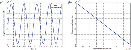
According to Equation(19)(19) $\left(\begin{array}{c}u\\ \theta \end{array}\right)=\left[\begin{array}{c}1/21/2\\ 1/2L-1/2L\end{array}\right]\left(\begin{array}{c}{\delta }_1\\ {\delta }_2\end{array}\right)$(19) , the system’s mass matrix and stiffness matrix in the $\left(u,\theta \right)$ plane do not include coupling terms; the system has an analytical solution. The vibration equation is solved using the findings of the preceding section, and the displacement response of the system under transverse impact is illustrated in Figure 12. As seen in this figure, the system’s vibration is a conventional undamped linear free vibration. Due to the same tension and compression stiffness of the springs, the mass can only spin in the plane during the transverse impact, i.e., the transverse reaction, which implies that the system’s initial angular velocity can only induce rotational vibration at this moment. The transverse impact causes only corner deformation; no axial deformation occurs. The following conditions are used in the calculation: the spring stiffness coefficient is a = 22,102 × 10³N/m, the system mass is m = 1000 Kg, the connecting cylindrical shell radius is L = 1 m, and the connecting cylindrical shell mass is J = 2500 Kg∙m². The system transverse starting velocity is ${\dot{\theta }}_0=1rad/s$.

Figure 12. The vibration response of the mass-spring two-degree-of-freedom system when the spring stiffness is constant: (a) Displacement response and (b) In-plane response of spring displacement.

7.2. Tension and compression stiffness nonlinear spring vibration response ( $\mathit{k}=2a\delta +b$)

According to Equation (22)(22) $\left[\begin{array}{c}m\\ 0\end{array}\right.\left.\begin{array}{c}0\\ J\end{array}\right]\left(\begin{array}{c}\ddot{u}\\ \ddot{\theta }\end{array}\right)+\left[\begin{array}{c}{k}_1^{\ast }+k_2^{\ast }\\ L\left(k_1^{\ast }-k_2^{\ast }\right)\end{array}\right.\left.\begin{array}{c}L\left(k_1^{\ast }-k_2^{\ast }\right)\\ L^2\left(k_1^{\ast }+k_2^{\ast }\right)\end{array}\right]\left(\begin{array}{c}u\\ \theta \end{array}\right)=0$(22) , the mass matrix of the system is symmetric between the generalized coordinates ${\delta }_1$ and ${\delta }_2$, the components are specified, and the stiffness matrix of the system is diagonal. When $m{L}^2=J$, the mass matrix is diagonal and the equations are uncoupled; when $m{L}^2\ne J$, the mass matrix is symmetric and the equations are inertially coupled.

When the equations are decoupled, the generalized coordinates and vibration become independent, and the system’s stiffness matrix becomes nonlinear. The nonlinear vibration equation (22)(22) $\left[\begin{array}{c}m\\ 0\end{array}\right.\left.\begin{array}{c}0\\ J\end{array}\right]\left(\begin{array}{c}\ddot{u}\\ \ddot{\theta }\end{array}\right)+\left[\begin{array}{c}{k}_1^{\ast }+k_2^{\ast }\\ L\left(k_1^{\ast }-k_2^{\ast }\right)\end{array}\right.\left.\begin{array}{c}L\left(k_1^{\ast }-k_2^{\ast }\right)\\ L^2\left(k_1^{\ast }+k_2^{\ast }\right)\end{array}\right]\left(\begin{array}{c}u\\ \theta \end{array}\right)=0$(22) may be numerically solved using MATLAB’s ODE solver, and the system’s time course response in generalized coordinates ${\delta }_1$ and ${\delta }_2$ can be derived. The derived values of and response are included into equation (20)(20) $\left\{\begin{array}{c}{k}_1=2a{\delta }_1+b\\ k_2=2a{\delta }_2+b\end{array}\right.$(20) , and the system’s vibration response in the $\left(u,\theta \right)$ plane may be determined through matrix operation. Figure 13 illustrates the system’s axial and lateral displacement responses, as well as its velocity response, upon lateral impact. The circumstances are as follows: the spring stiffness coefficient are $a=-26481\times {10}^{3}N/m,b=25297\times {10}^{3}N/m$, the mass of the system is m = 1000 Kg, the connecting cylindrical shell radius is L = 1 m, J = 1000 Kg∙m² and the starting lateral velocity of the system is ${\dot{\theta }}_0=1rad/s$. 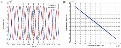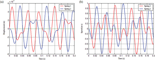As seen in Figure 13, when the spring stiffness is proportional to displacement, the system exhibits not only transverse but also axial vibration in response to transverse shock. The system’s vibration is stable, always in the planes I, II, and IV, and the vibrations of springs 1 and 2 are independent of one another, as seen in Figure 14.

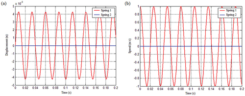
Figure 13. The vibration response of the system under the condition that the spring stiffness is a linear function of displacement and the mass matrix is not coupled: (a) Displacement response and (b) Speed response.

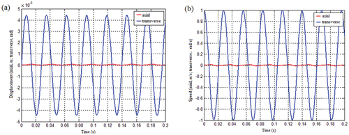
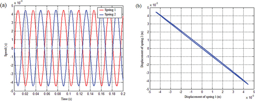
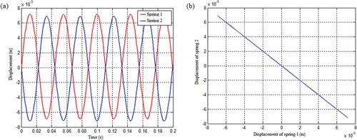
Figure 14. The displacement response of spring 1 and spring 2 under the condition that the mass matrix of spring stiffness is a linear function of displacement is not coupled: (a) Displacement response of springs and (b) The displacement response of springs when the initial angular velocity is 1 rad/s.

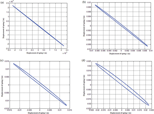
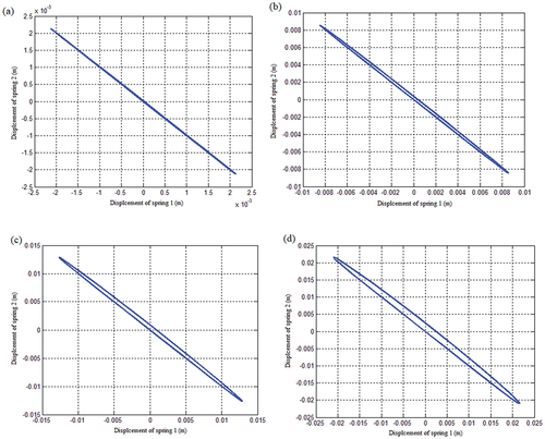
When the spring’s axial stiffness is a linear function of the axial displacement and the mass matrix contains no coupling factor, Figure 15 illustrates the effect of various beginning transverse rotation angular velocities on the system motion area. When the initial angular velocity is minimal, the system travels in the II and IV regions of the $\left(u,\theta \right)$ plane; when the initial angular velocity is more than 1 rad/s, the system moves in the I, II, and IV areas of the $\left(u,\theta \right)$ plane, illustrating the system’s movement. The location is associated with the original circumstances.

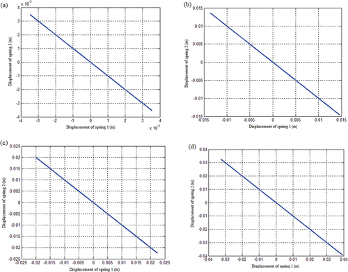
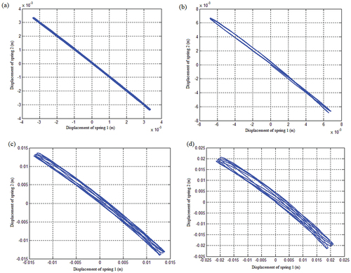
Figure 15. The vibration response of the system in the $\left(u,\theta \right)$ plane, under the condition that the spring stiffness is a linear function of displacement and the mass matrix of the system is not coupled, when the initial angular velocity is (a) 0.5 rad/s, (b) 2 rad/s, (c) 3 rad/s, and (d) 5 rad/s.

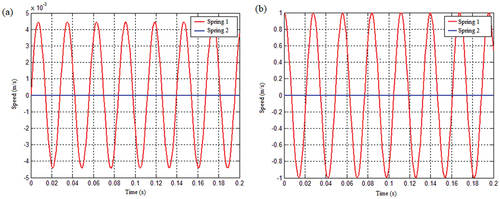
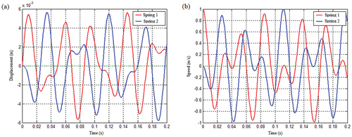
To demonstrate that the mass matrix is not coupled, spring 1 and spring 2 have separate vibrations. At this point, given just spring 1’s starting velocity, i.e., the ${\dot{\delta }}_1\ne 0$ condition, the vibration displacement and velocity responses of spring 1 and spring 2 are produced as shown in Figure 16. As seen in the figure, the vibration responses of springs 1 and 2 are fully independent owing to the equation’s decoupling.

Figure 16. Vibration response of spring 1 and spring 2 under the condition that the mass matrix of the system with a given initial velocity of spring 1 is not coupled: (a) Displacement response and (b) Speed response.

When the equations cannot be decoupled upon transverse impact, the vibrations of generalized coordinates ${\delta }_1$ and ${\delta }_2$ become connected. At this stage, the nonlinear vibration Equation (20)(20) $\left\{\begin{array}{c}{k}_1=2a{\delta }_1+b\\ k_2=2a{\delta }_2+b\end{array}\right.$(20) may be numerically solved using MATLAB’s ODE solver, and the system’s time-history response in generalized coordinates ${\delta }_1$ and ${\delta }_2$ can be obtained. By including the findings of and into Equation (20)(20) $\left\{\begin{array}{c}{k}_1=2a{\delta }_1+b\\ k_2=2a{\delta }_2+b\end{array}\right.$(20) , the system’s vibration response in the $\left(u,\theta \right)$ plane may be determined by matrix operation. Figure 17 illustrates the system’s axial and transverse displacement responses, as well as its axial and transverse velocity responses, after a transverse impact. The following circumstances are used in the calculation: the spring stiffness coefficients are $a=-26481\times {10}^{3}N/m,b=25297\times {10}^{3}N/m$, the system mass is m = 1000 Kg, the connecting cylindrical shell radius is $L=1m,J=2500Kg\cdot m^2$, and the system transverse starting velocity is ${\dot{\theta }}_0=1rad/s.$ As seen in Figure 17, when the spring stiffness is a linear function of displacement and the mass matrix exhibits inertial coupling, the system produces only transverse vibration in response to transverse impact, without producing axial vibration, and the system’s vibration is stable. The system is always in zone II or IV of the $\left(u,\theta \right)$ plane, as seen in Figure 18, ${\delta }_1⟨0,{\delta }_2⟩0or{\delta }_1>0,{\delta }_2<0.$

Figure 17. Vibration response of the system under the coupling condition of the linear function mass matrix with spring stiffness as displacement: (a) displacement response and (b) Speed response.

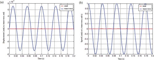
Figure 18. Displacement response of spring 1 and spring 2 under the coupling condition of the mass matrix with a linear function of spring stiffness as displacement: (a) Displacement response of spring 1 and spring 2 and (b) Displacement response of spring 1 and spring 2 when the initial angular velocity is 1 rad/s.

When the spring’s axial stiffness is a linear function of the spring’s axial displacement and the mass matrix includes coupling terms, Figure 19 illustrates the effect of various starting transverse rotation angular velocities on the system’s motion area. As can be observed, regardless of the initial angular velocity, the system will move in the II and IV sections of the $\left(u,\theta \right)$ plane, indicating that the system’s motion region is independent of the beginning circumstances at this moment.

Figure 19. The displacement response of the spring in the $\left(u,\theta \right)$ plane under the coupling condition of the mass matrix of the linear function the system with spring stiffness as displacement when the initial angular velocity is (a)0.5 rad/s, (b)2 rad/s, (c)3 rad/s, and (d)5 rad/s.

To demonstrate the mass matrix’s coupling, the vibrations of springs 1 and 2 are coupled. At this point, given simply the starting velocity of spring 1, under the condition of ${\dot{\delta }}_1\ne 0$, the vibration displacement and velocity responses of spring 1 and spring 2 are derived as illustrated in Figure 20. As seen in this figure, the vibration response of the produced springs 1 and 2 are linked, that is, spring 1 causes spring 2 to vibrate, and the vibration of the two springs is stable at this moment.

Figure 20. The vibration response of the spring under the coupling condition of the mass matrix of the system with the given initial velocity of spring 1: (a) Displacement response and (b) Speed response.

7.3. Vibration response of tension and compression bilinear stiffness spring (bilinear simplified model $k=\left\{\begin{array}{c}a,\delta >0\\ b,\delta <0\end{array}\right)$

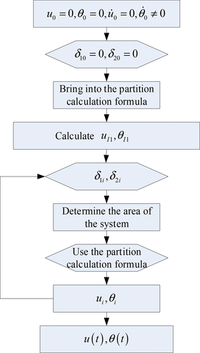
For bilinear stiffness, the system’s motion under lateral impact includes all partitions in the plane, and the system’s stiffness matrix is dependent on the system’s state of motion in the $\left(u,\theta \right)$ plane. To begin, we determine the vibration region corresponding to the system at this time using the system’s initial conditions, and then calculate the initial deformation of the two springs using the partition formula to obtain the system’s displacement in that time step. Finally, we perform matrix operations to obtain the deformation of the two springs in that time step. The system is then assessed to be in the area again using the system partition map, and the analytical solution in that region is called to acquire the system’s displacement, which is then recursively called to produce the system’s response within the predicted time step. As seen in Figure 21, this procedure may be done using MATLAB software programming.

Figure 21. The calculation process of the mechanism model under the bilinear stiffness axial and transverse coupled impact.

Figure 22 illustrates the system’s axial and transverse displacement responses, velocity responses, and vibration phase diagrams under transverse impact. The spring tensile stiffness is $a=19045\times {10}^{3}N/m$, the compression stiffness is $b=29130\times {10}^{3}N/m$, the system mass is m = 1000 Kg, the flange connection cylinder shell radius is $=1m,J=2500Kg\cdot m^2$, ${\dot{\theta }}_0=1rad/s$. As seen in Figure 22, when the spring tension and compression stiffness are bilinear, the system produces not only transverse but also axial vibration in response to the transverse impact. The system’s vibration is similarly stable, and it always travels in zones I, II, and IV of the $\left(u,\theta \right)$ plane, as seen in Figure 23, specifically, ${\delta }_1\ge 0,{\delta }_2\ge 0,{\delta }_1⟨0,{\delta }_2⟩0and{\delta }_1>0,{\delta }_2<0$.

Figure 22. The spring stiffness is the vibration response of the system under the condition of bilinear tension and compression: (a) Axial and transverse vibration displacement response and (b) Axial and transverse vibration speed response.

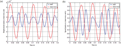
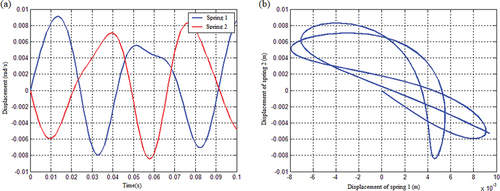
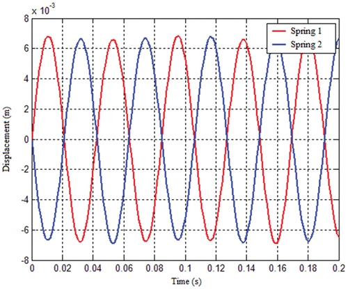
Figure 23. The spring stiffness is the vibration response of the spring under the condition of bilinear tension and compression: (a) Displacement response and b) Displacement relationship.

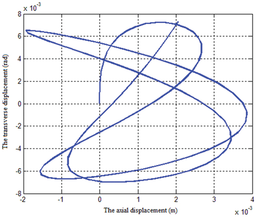
Figure 24 illustrates the system’s vibration response in the axial and transverse displacement planes after a transverse impact. As seen in Figure 23(a), the system always travels in the $\left(u,\theta \right)$ plane’s I, II, and IV zones and never enters zone III; this is another critical property of the bilinear system with spring tension and compression stiffness that corresponds to Figure 23(b).

Figure 24. Vibration response of the system in the axial and transverse planes.

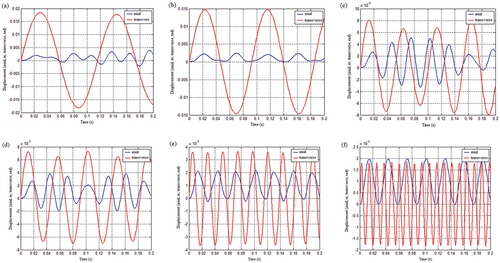
The radius of the flange connection cylinder shell L has a negligible effect on the axial vibration frequency of the system, but a significant effect on the transverse vibration frequency. To demonstrate this, the connecting cylinder shell radius L is varied under the same calculation circumstances, yielding the system’s axial and transverse vibration displacement responses illustrated in Figure 25. It can be seen from the figure that the influence of L on the axial vibration frequency is relatively small and almost has no influence, while the influence of L on the transverse vibration frequency is relatively large. The multiple of the rise in L is the increase in the transverse vibration frequency; that is, the transverse vibration frequency increases in lockstep with the increase in L.

Figure 25. Axial and transverse displacement response of tension and compression bilinear stiffness spring of the connecting cylindrical shell radius L: (a) L = 0.4, (b) L = 0.5, (c) L = 0.9, (d) L = 1, (e) L = 2 and (f) L = 4.

7.4. Nonlinear stiffness spring vibration response (stiffness is a quadratic function of displacement $\mathit{k}=3a{\delta }^2+2b\delta +c$)

By observing Equation (25)(25) $\mathbf{y}=A{e}^{\left(\omega t+\varphi \right)i}$(25) , the system’s mass matrix remains symmetric, and the diagonal elements are determined; also, when $m{L}^2=J$, the mass matrix becomes a diagonal matrix, and the equations become decoupled. When $m{L}^2\ne J$, the mass matrix is symmetric, and inertial coupling exists between the equations.

When the equations are decoupled for transverse impact, the generalized coordinates and vibration are independent of one another, and the system’s stiffness matrix is nonlinear. The nonlinear vibration Equation (20)(20) $\left\{\begin{array}{c}{k}_1=2a{\delta }_1+b\\ k_2=2a{\delta }_2+b\end{array}\right.$(20) is numerically solved using MATLAB’s ODE solver. The system’s time history response in generalized coordinates ${\delta }_1$ and ${\delta }_2$ may be determined. By including the findings of and into Equation (20)(20) $\left\{\begin{array}{c}{k}_1=2a{\delta }_1+b\\ k_2=2a{\delta }_2+b\end{array}\right.$(20) , the system’s vibration response in the $\left(u,\theta \right)$ plane may be determined by matrix operation. Figure 26 illustrates the system’s axial and transverse displacement responses, as well as its axial and transverse velocity responses, after a transverse impact. The following circumstances are used in the calculation: the spring stiffness coefficients are $a=-66720\times {10}^{3}N/m,b=-19019\times {10}^{3}N/m$, $c=27478\times {10}^{3}N/m$, the system mass is m = 1000 Kg, the connecting cylindrical shell radius is $L=1m,J=1000Kg\cdot m^2$, and the system transverse initial velocity is ${\dot{\theta }}_0=1rad/s$. As seen in Figure 26, when the spring stiffness is a linear function of displacement, the system produces only transverse vibration in response to the transverse impact, and no axial vibration. The system’s vibration is steady, and it is always in the II and IV regions of the (u,) plane. As seen in Figure 27, 1 > 0, 2 > 0 or 1 > 0, 2 > 0.

Figure 26. Vibration response of the system under the uncoupled condition of quadratic function mass matrix with spring stiffness as displacement: (a) Axial and transverse displacement response and (b) Axial and transverse velocity response.

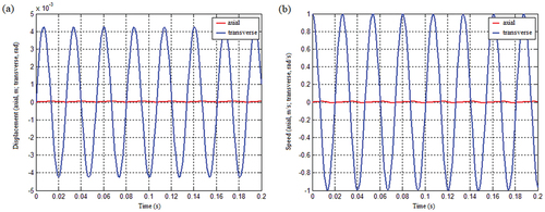
Figure 27. The spring displacement response under the condition that the spring stiffness is the quadratic function of displacement and the mass matrix is not coupled: (a) Displacement response of spring 1 and spring 2 and (b) The displacement response of the spring when the initial angular velocity is 1 rad/s.

When the spring’s axial stiffness is a quadratic function of the axial displacement and the mass matrix contains no coupling factor, Figure 28 illustrates the effect of various starting transverse rotation angular velocities on the system motion area. As can be observed, when the first angular velocity is minimal, the system travels in the II and IV regions of the $\left(u,\theta \right)$ plane; when the initial angular velocity is more than 1 rad/s, the system moves in the I, II, and IV regions of the $\left(u,\theta \right)$ plane, indicating that the beginning circumstances are connected.

Figure 28. The displacement response of the spring in the $\left(u,\theta \right)$ plane under the condition that the mass matrix of the quadratic function system with spring stiffness as displacement is not coupled, when the initial angular velocity is (a) 0.5 rad/s, (b)2 rad/s, (c)3 rad/s, and (d) 5 rad/s.

To demonstrate that the mass matrix is not connected, spring 1 and spring 2 have separate vibrations. At this point, given just spring 1’s starting velocity, i.e., condition ${\dot{\delta }}_1\ne 0$, the vibration displacement and velocity responses of spring 1 and spring 2 are produced as illustrated in Figure 29. As seen in this figure, the vibration responses of springs 1 and 2 are independent owing to the equation’s decoupling.

Figure 29. The vibration response of spring 1 and spring 2 under the condition of an uncoupled mass matrix of a quadratic function with spring stiffness as displacement: (a) Spring displacement response and (b) Spring speed response.

When the equations cannot be decoupled during transverse shock, vibrations of the generalized coordinates ${\delta }_1$ and ${\delta }_2$ become connected. The nonlinear vibration Equation(25)(25) $\mathbf{y}=A{e}^{\left(\omega t+\varphi \right)i}$(25) may be numerically solved using MATLAB’s ODE solver, and the time course response of the system under the generalized coordinates ${\delta }_1$ and ${\delta }_2$ can be derived. By including the findings of and into Equation (20)(20) $\left\{\begin{array}{c}{k}_1=2a{\delta }_1+b\\ k_2=2a{\delta }_2+b\end{array}\right.$(20) , the system’s vibration response in the $\left(u,\theta \right)$ plane may be determined by matrix operation. At this stage, Figure 30 illustrates the system’s axial and transverse displacement responses, as well as its axial and transverse velocity responses to transverse impact. The following conditions apply to the calculation: $a=-26481\times {10}^{3}N/m,b=25297\times {10}^{3}N/m$, m = 1000 Kg, L = 1 m, J = 2500 kg∙m². As seen in Figure 30, when the spring stiffness is a linear function of displacement and the mass matrix is coupled inertially, the system produces not only transverse vibration but also axial vibration in response to the transverse impact. The system’s vibration is also stable, and it always vibrates in regions I, II, and IV of the $\left(u,\theta \right)$ plane, as seen in Figure 31, specifically, 1 > 0, 2 > 0, or 1 > 0, 2 > 0.

Figure 30. The response of the system under the coupling condition of the quadratic function mass matrix with spring stiffness as displacement: (a) Displacement response and (b) Speed response.

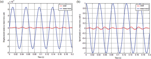
Figure 31. Spring displacement response under the coupling condition of quadratic function mass matrix with spring stiffness as displacement.

The impact of varying starting transverse rotation angular velocities on the system motion area is shown in Figure 32 when the spring’s axial stiffness is a quadratic function of the axial displacement and the mass matrix includes coupling terms. As can be observed, when the initial angular velocity is low, the system travels in the II and IV regions of the $\left(u,\theta \right)$ plane; when the initial angular velocity is high, the system moves in the I, II, and IV areas of the $\left(u,\theta \right)$ plane. This demonstrates that the system’s area of motion is dependent on the beginning circumstances.

Figure 32. The displacement response of the spring in the $\left(u,\theta \right)$ plane under the coupling condition of the mass matrix of the quadratic function system with spring stiffness as displacement, when the initial angular velocity is (a) 0.5 rad/s, (b) 1 rad/s, (c) 2 rad/s, and (d) 3 rad/s.

To demonstrate the mass matrix’s coupling, the vibrations of springs 1 and 2 are coupled. At this point, given just spring 1’s starting velocity,$\stackrel{\ne }{{\delta }_1}0$, the vibration displacement and velocity response of spring 1 and spring 2 are produced as illustrated in Figure 33. As seen in the figure., the obtained vibration responses of springs 1 and 2 are linked, i.e., spring 1 causes spring 2 to vibrate, and the vibration of the two springs is likewise stable at this moment.

Figure 33. The spring vibration response under the coupling condition of quadratic function mass matrix with spring stiffness as displacement: (a) Displacement response and (b) Speed response.

8. Experimental verification of nonlinear dynamic response of the bolted flange joint

To validate the rationale and efficacy of the reduced nonlinear dynamic model, an impact test was conducted on the typical bolt-flange-gasket connection structure under consideration, and test data were gathered and processed to check and confirm the calculation model.

8.1. Axial knock response test

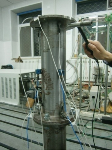
The test uses the LMS Test. Lab 9B test system was developed by Belgium. This test makes use of the module for shock vibration testing, namely the hammer impulse shock test. Bolts on the ground secure the axial bottom of the test composite construction. A hammer is used to produce axial pounding on the bolted flange joint during the dynamic test, and the structure’s reaction is measured using an acceleration sensor. Figure 34 depicts the experimental test arrangement. The best placement for the excitation point is one with a high rigidity that can excite all modes. The precise position is shown in Figure 35. The arrangement of the measurement points is largely determined by these points: to represent the fundamental form and properties of the complete bolted flange joints, the measuring points are rotated 90 degrees around the flange axis, and nodes are avoided as much as feasible. The precise locations are shown in Figure 35. Within one second of the initiation of the tap, the test collects the acceleration response data. The system’s sample frequency is set to 6000 Hz, and the data is sent to a Dell Latitude D600 laptop computer. Each percussion was repeated three to five times to confirm the stability of the test environment and circumstances; the hammer struck the structure in a triangle pattern, which was recorded by the front end of DK3038.

Figure 34. Experimental test layout.

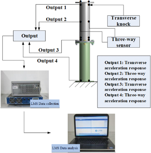
Figure 35. Experimental picture.

8.2. Analysis of test results

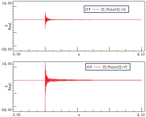
The bottom end of the bolted flange joint is fully bolted, and the top end is subjected to a transverse impact load. Calculate the transient dynamic response of the test specimen’s bolted flange joint under lateral impact load. The rigidity of the linked pieces exceeds that of the junction (Mao and Li 2018). Figure 36 illustrates the outcome. The top of the bolted flange joint also generated axial and transverse responses, with the transverse response amplitude being bigger than the axial response amplitude, which was consistent with the mechanism model’s predicted findings under the transverse stress. That is, when the transverse impact occurred, the bolted flange joint generated linked horizontal and vertical vibration. Additionally, the bolted flange joint’s vibration is dampened, i.e., the structural damping and contact damping of the bolted flange joint should be included while developing the bolted flange joint’s nonlinear vibration mechanism model and nonlinear simplified dynamic simulation calculation model.

Figure 36. Vibration acceleration response of the bolted flange joint under the transverse impact (the upper picture is axial; the lower picture is transverse).

9. Conclusion

1) When the spring stiffness is constant and the stiffness is a linear function of displacement, and the mass matrix of the vibration control equation is coupled, only transverse corner vibration is generated in the bolted flange joint under transverse load. When the spring axial stiffness is a primary function of displacement and the mass matrix of the vibration control equation is not coupled or when the spring stiffness is bilinear and the stiffness is a quadratic function of displacement, the combined structure produces transverse and axial coupled vibration (He 2015).

2) Whatever the spring stiffness is reduced to, the transverse or transverse and axial movements of the system are all periodic vibrations, and the phase diagram of the system motion demonstrates that the vibration state is stable.

3) Regardless of how simple the spring stiffness is, the system’s vibration response under transverse impact is dependent not only on the system’s quality but also on the radius L of the connecting cylinder shell. Particularly when the spring stiffness is bilinear, L has a little effect on the axial vibration frequency of the system; however, L has a significant effect on the transverse vibration frequency of the system, and the transverse vibration frequency changes linearly with L.

Disclosure statement

No potential conflict of interest was reported by the author(s).

Additional information

Funding

This work was supported by the The youth project of science and technology research program of Chongqing Education Commission of China [KJQN201901113]; The Open Foundation of Key Laboratory of Modern Measurement & Control Technology (Beijing Information Science and Technology University), Ministry of Education [KF20211123201]; The Natural Science Foundation of Chongqing [cstc2021jcyj-msxmX0440]; The China Postdoctoral Science Foundation funded project [2019M663443].

References

- Abid, M. 2008. HUSSAIN S.Gasketed Joint’s Relaxation Behaviour during Assembly Using Different Gaskets: A Comparative Study[M]//Advanced Design and Manufacture to Gain A Competitive Edge.Berlin, 91–100. Germany: Springer.
- Ahmadian, H., M. Ebrahimi, J. E. Mottershead, and M. I. Friswell. 2002. “Identification of bolted-joint Interface Model.” Proceedings of ISMA2002: International Conference on Noise and Vibration Engineering, Katholieke University, Leuven Belgium, pp. 1741–1748.
- Ahmadian, H., and H. Jalali. 2007. “Generic Element Formulation for Modeling Bolted Lap joints[J].” Mechanical Systems & Signal Processing 21 (5): 2318–2334. doi:10.1016/j.ymssp.2006.10.006.
- Alkatan, F., P. Stephan, A. Daidie, J. Guillot, et al. 2007. “Equivalent Axial Stiffness of Various Components in Bolted Joints Subjected to Axial loading[J].” Finite Elements in Analysis and Design 43 (8): 589–598. doi:10.1016/j.finel.2006.12.013.
- Butner, C., D. Adams, and J. R. Foley. 2012. Simplified Nonlinear Modeling Approach for a Bolted Interface Test Fixture[M]// Topics in Nonlinear Dynamics. Vol. 3. New York: Springer.
- Chen H. , Xiang, J. , Zuo, Z. , & He, L. et al. 2018. “Non-Linear Characters of Stiffness of Combination Structure Based on Equivalent Model[J].” Journal of Tianjin University 51 (2): 190–195.
- de Lima, L. R. O., J. L. Freire, F. de, P. C. G. Vellasco, S. da, S. A. L. D. Andrade, J. G. S. D. Silva, et al. 2009. “Structural Assessment of Minor Axis Steel Joints Using Photoelasticity and Finite Elements[J].” Journal of Constructional Steel Research 65 (2): 466–478. doi:10.1016/j.jcsr.2008.01.030.
- Gia Ninh, D., V. Ngoc Viet Hoang, and V. Le Huy. 2021. “A New Structure Study: Vibrational Analyses of FGM convex-concave Shells Subjected to electro-thermal-mechanical Loads Surrounded by Pasternak Foundation.” European Journal of Mechanics - A/Solids 86 (104168): 09977538. doi:): 09977538. doi:10.1016/j.euromechsol.2020.104168.
- He, L. G. 2015. Study of Nonlinear Mechanical Behavior of Assembly Structure with Bolted Joints in Diesel Engine design[D]. Beijing: Beijing Institute of Technology.
- Hoang, V., V. Ngoc, D. Gia Ninh, V. T. Thang, D. V. Truong, et al. 2021. “Nonlinear Dynamics of Functionally Graded Graphene Nanoplatelet Reinforced Polymer Doubly-Curved Shallow Shells Resting on Elastic Foundation Using a Micromechanical Model”. Journal of Sandwich Structures & Materials 23 (7): 3250–3279. doi:10.1177/1099636220926650.
- Lehnhoff, T. F., K. I. Ko, and M. L. McKay. 1994. “Member Stiffness and Contact Pressure Distribution of Bolted Joints[J].ASME.” Journal of Mechanical Design 116 (2): 550–557. doi:10.1115/1.2919413.
- Luan, Y. 2012. Study on Dynamic Modeling of Bolted Flange Connections in Aerospace Structures[D]. Liao Ning: Dalian University of Technology.
- Luan, Y. , Guan, Z. Q., Cheng, G. D., & Liu, S., et al. 2013. “A simplified Nonlinear Dynamic Model for the Analysis of Pipe Structures with Bolted Flange joints[J].” Journal of Sound and Vibration 331 (2): 325–344. doi:10.1016/j.jsv.2011.09.002.
- Mao, K. M., and B. Li. 2018. Modeling and Application of Joint Son Machine Tools[M]. Wuhan: Wuhan university of science and technology press.
- Meng, C. X. , Zhang, W. S. , Hui, M. A. , Qin, Z. Y. , & Fan, F. Y. 2019. “analysis of Dynamic Characteristics of a Bolted Drum Rotor structure[J].” Journal of Vibration Engineering (3).
- Nassar, S. A. 2009. “Novel Formulation of Bolt Elastic Interaction in Gasketed Joints[J].ASME“. Journal of pressure vessel technology . 10: 051204.
- Pereira, E. N., M. B. H. Mantelli, and F. H. Milanez. “Statistical Model for Pressure Distribution of A Bolted Joint[C].” Washington: 40th Thermo physics Conference, 2008.
- Takaki, T., and T. Fukuoka. 2003. “Finite Element Simulation of Bolt-Up Process of Pipe Flange Connections with Spiral Wound Gasket[J].ASME.” Journal of Pressure Vessel Technology 125 (4): 371–378. doi:10.1115/1.1613304.
- Vadean, A., D. Leray, and J. Guillot. 2006. “Bolted Joints for Very Large bearings-numerical Model development[J].” 42 (4): 298–313.
- Wang, J. M., G. D. Li, and W. Y. Huang. 2006. “The Research for the Dynamic Characteristics of the Missile with the Jointed Structure by the Test Method[J].” Structure & Environment Engineering 33 (1): 52–58.
- Wei, H. T. , Kong, X. R. , Wang, B. L. , & Zhang, X. M. et al. 2014. “Non-Linear Dynamic Response of a Beam with Bolted Joint Based on Modal Shape Transfer[J].” Journal of Vibration and Shock 12 (33): 42–47.
- Williams, G. J., A. R. E, N. D. H, T. G. F. Gray, et al. 2009. “Analysis of Externally Loaded Bolted Joints: Analytical, Computational and Experimental study[J].” International Journal of Pressure Vessels & Piping 86 (7): 420–427. doi:10.1016/j.ijpvp.2009.01.006.
- Yin, Y. H. 2008. “Relations between Internal Forces and Deformation of a Bolt Joint with Their Application to Design Based on 3d Fem Simulation[J].” Journal of Mechanical Strength 30 (6): 947–952.
- Zhang, Q. Y. 2003. Fuzzy Reliability Analysis for A Flanged Connection System of Rocket Motors[D]. Shan xi: Northwestern Polytechnical University.