
 ?Mathematical formulae have been encoded as MathML and are displayed in this HTML version using MathJax in order to improve their display. Uncheck the box to turn MathJax off. This feature requires Javascript. Click on a formula to zoom.
ABSTRACT
Nowadays, the process of urbanization is accelerating, and the density of buildings is increasing rapidly. Natural ventlation is an energy-saving way of building ventilation and to solve the issue of building overheating. The buildings are all considered as cubes and their arrays are evenly distributed. The results from nearly 100 cases show density is the main factor in uniform arrays and not much difference between the staggered and normal arrangements if consider a year. The method can reflect the ventilation capacity of the buildings, which is somewhat inverse to the air age but different meaning. It can be used to guide the layout and planning in early design stage.
1. Introduction
Building energy-saving technologies can improve energy efficiency and reduce carbon emissions, among which natural ventilation is an effective means. Natural ventilation can improve indoor air quality and reduce air conditioning energy consumption. (Wang et al. Citation2022; Zhang et al. Citation2022) Its driving forces are divided into buoyancy (Wei et al. Citation2010) and wind pressure ventilations. (Zhang et al. Citation2021) The potential for wind pressure ventilation is mainly determined by climatic conditions and building design; the latter includes building height, density, and arrangement. (Yin et al. Citation2010) In this study, we discuss the effect of building arrangement on the natural ventilation potential (VP) of wind pressure. There are three main research methods for building wind environments: field tests, wind tunnel experiments, and computational fluid dynamics (CFD).
The CFD simulation method, whose accuracy has been demonstrated in numerous studies, is widely used in the study of wind environments around buildings. In a study of complex urban canopies, Ricci et al. (Citation2020) observed that the fluid field under different Reynolds-averaged Navier – Stokes (RANS) equation models can differ by 20–60%. van Hooff, Blocken, and Tominaga (Citation2017) observed that all RANS models underestimated the turbulent kinetic energy, however, large eddy simulations (LES) provided better simulation results for the average velocity and turbulent kinetic energy. Van Hooff and Blocken (Citation2020) found that the RNG k-ε turbulence model in predicting mixing ventilation flows; differences in mean velocity were generally within 10–20%, while 80% of the predictions of TKE were within 30% from the measurement results. Hang et al. (Citation2013) observed that the standard k–ε outperforms other RANS models in airflow simulations of street canyons. Shirzadi, Naghashzadegan, and Mirzaei (Citation2018) quantified the limitations of the RANS model in the application of ventilation in highly congested urban areas and observed that the accuracy of the RANS model was better when the building densities were between 0.25 and 0.4. Tominaga et al. (Citation2004) compared the standard k–ε model, revised k–ε models, differential stress model, Large Eddy Simulation, and direct numerical simulation with the experimental results and observed that the prediction of the horizontal scalar velocity distribution of pedestrians was consistent with the measured results in the actual building group, except in the wake region and far away outside the area of the target building because the grid resolution was not sufficiently fine. Montazeri and Blocken (Citation2013) studied the influence of balconies on the wind pressure coefficient and observed that for mid-rise buildings with or without balconies, the RANS simulation was biased when the wind was oblique. All other cases were consistent with the wind tunnel experiments. Therefore, the above study shows that the CFD simulation method can reproduce the wind tunnel experimental results and can be used to predict the airflow field around the building.
For a single building, there are various factors affecting natural ventilation, such as outdoor wind direction and wind speed, building opening area and position, outer surface protrusion, and roughness. Derakhshan and Shaker (Citation2017) explored the effect of the opening aspect ratio on indoor ventilation and observed that when the outdoor wind direction was greater than 45°, the ventilation volume was unrelated to the window size. Mattsson (Citation2004) studied the influence of terrain, surrounding environment, and wind speed on the ventilation rate. For high-rise buildings, Liu et al. (Citation2019) observed that the ventilation is extremely sensitive to the changes in wind conditions, followed by the difference in ventilation mode, window type, and window orientation. Chand, Bhargava, and Krishak (Citation1998) observed that balconies changed the wind-pressure distribution on the windward wall. Lee et al. (Citation2015) observed that the change in the shape of the outer louver had a significant impact on the natural ventilation rate. Ok, Yasa, and Özgunler (Citation2008) suggested that openings located on perpendicular surfaces increase the airflow velocity within courtyards. Kindangen, Krauss, and Depecker (Citation1997) studied the effect of roof shape on indoor ventilation and observed that enhancing negative pressure can promote indoor air circulation. The design of a single building mainly affects indoor ventilation and has less impact on the outdoor wind environment. The outdoor wind environment is mainly affected by local meteorological data and building arrangements.
The proliferation of density in urban residential areas has led to many wind environment problems in urban residential areas, such as poor ventilation and difficulties in pollutant diffusion. Some studies have shown that reasonable spatial design and configuration of urban residential areas can significantly improve the wind environment of residential areas. Zhen et al. (Citation2019) and Asfour (Citation2010) believed that the spatial form of urban residential blocks was the main factor affecting the wind environment around buildings. Kim, Yoshida, and Tamura (Citation2012) observed through wind tunnel experiments that when the building density was high, the average wind speed between buildings decreased significantly and turbulence intensity increased significantly. Through wind tunnel experiments, Tsutsumi, Katayama, and Nishida (Citation1992) observed that the spacing in buildings have a greater impact on the building wind pressure coefficient, and with the change in building density, the wind pressure coefficient distribution on the building surface will be larger in the central area than in the surrounding area. Ling Chen, Lu, and Yu (Citation2017) found that the influence of terrain factors on building ventilation cannot be ignored in densely built mountain areas, and the ventilation capacity of open space in urban areas is better than that in narrow areas. Based on three buildings, Dai, Mak, and Ai (Citation2019) found that the existence of upstream buildings does not necessarily make the wind environment of downstream buildings worse. Hanna et al. (Citation2002) observed that compared with staggered arrays, the canyon effect of a normal arrangement is more obvious. Al-Sallal, AboulNaga, and Alteraifi (Citation2001) observed that changing building heights upstream and downstream had a greater impact on the airflow path and velocity in urban spaces. Wang and Ng (Citation2018) observed that the ventilation effect in rectangular buildings was better than that in square buildings. Arkon and Özkol (Citation2014) observed that the block shape demonstrates a significant influence on the wind speed at pedestrian heights in a survey. Hang, Li, and Sandberg (Citation2011) observed that density has a greater impact on high-rise building arrays and that wider streets can improve ventilation.
For the building layout, if the shape, porosity, and surface roughness of the building are discussed, the problem will become very complicated, so the building model needs to be simplified. In wind tunnel experiments, Buccolieri et al. (Citation2019) simplified buildings as cubes to ignore the effects of building shape and surface roughness. In this study, such an ideal building model is also taken. At the same time, when there are more building models, the method of evaluating the building ventilation potential by making the difference in wind pressure between the two sides of the building used in the previous study is considered to be cumbersome. We propose a method for evaluating the building ventilation potential based on the standard difference of wind pressure on the building façade and explored the effects of density, staggered and normal arrangement, and potential of wind-force natural ventilation.
In the study, we first introduced the building complex model and CFD settings and compare and validate them with the wind tunnel experimental data. Thereafter, the potential evaluation method based on the standard deviation of wind pressure was proposed. Next, the impact of building density, building arrangement, overhead, and year-round weather data were analyzed. Finally, a comparison with the conclusions of previous studies was presented.
2. Building models and methodology
2.1. Building model
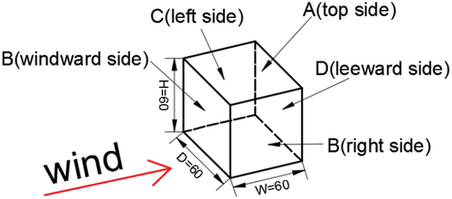
To measure the accuracy of wind tunnel experiments, Buccolieri et al. (Citation2019) and Hang and Li (Citation2010) established the ideal building group arrays where each building was simplified as a cube, whose overall dimensions were 0.06 × 0.06 × 0.06 m3 (length × width × height), as shown in . In this study, we built a CFD model based on the aforementioned model and its dimensions.
Figure 1. Building model.
2.2. CFD setting
2.2.1. Fluid domain
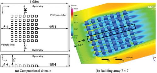
As suggested by Tominaga et al. (Citation2015), Blocken, Stathopoulos, and Carmeliet (Citation2007), and Franke et al. (Citation2007), the flow field was set as follows. The distance from the building to the top and sides of the computational domain was 5 H (H means the building height). The distances of the outlet boundary downstream of the building and inlet boundary upstream of the building are 15 H and 5 H, respectively. The resulting computational domain size was 1.98 × 1.38 × 0.36 m3(length × width × height), as shown in .
Figure 2. Building array and computational domain. (a) Computational domain, (b) Building array 7 × 7.
2.2.2. Boundary conditions and turbulence model
In the boundary conditions of ANSYS Fluent 2021, the ground and building surfaces were defined as walls, the top and sides of the fluid domain exhibited symmetric boundary conditions, the outlet was set as the pressure outlet, and the inlet was set as the velocity inlet. In the wind tunnel experiment (Buccolieri et al. Citation2019), the distribution of the measured inflow velocity in the vertical direction was expressed as a power function, as shown in EquationEquation (1)(1)
(1) .
where U(z)(m/s) and U(H)(5.2 m/s) are the average wind speeds at the building height z (m) and the reference height H = 0.06 m, respectively. The vertical distribution of the turbulent intensity of the incoming flow was expressed as a power function, as shown in EquationEquation (2)(2)
(2) .
where I(z) (m/s) and I(H) (27.6 m/s) are the turbulence intensity at building height z (m) and reference height H (m), respectively. The average incoming velocity and turbulence intensity formulas were programmed into a user-defined function (UDF) and imported into Fluent. The Reynolds number is 20,800, which reaches the fully turbulent state.
The number of grids was more than 6 million, and the simulation time using LES was about a month for each case by Intel Xeon 4-core processor (32-core when hyperthreading) is enabled. On the second hand, Tominaga et al. (Citation2004) found in a similar case that the difference between RANS and LES within the buildings complex is small. Their difference mainly occurs in the wake, which is not considered in the study. Considering the time cost and accuracy, this paper uses RANS for simulation. The building model of Hang et al. (Citation2013) is similar to that used in this study. Additionally, and Hang et al. (Citation2013) observed that the simulated data from the standard k-ε model in the RANS model were closest to the experimental values. Therefore, this paper also uses the Standard k-ε model to simulate. The control equations were discretized by the finite volume method under the second order, the SIMPLEC scheme was used to couple pressure and velocity, and all residuals were at least 10−5 to convergence, and the computation time for all models is approximately 6 months.
2.2.3. Grid and sensitivity analyses
A schematic of the 7 × 7 array is shown in , and its meshing method is discussed in this section. According to the surface mesh technique of van Hooff and Blocken, (Citation2013), the grids were hexahedral structured grids with the quality ranging between 0.95 and 1. To control the number of grids, the surface and corners of the building were densified, as shown in .
Figure 3. Meshing of fluid domain. (a) Building array 7 × 7 and distance, (b) Grid between building, (c) Mesh of the entire area, (d) Mesh density at the edge of the building.
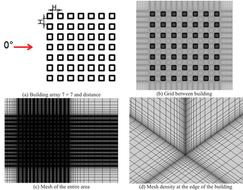
Seven densities were set: 0.01 m (minimum grid size; total number of grids = 140,000), 0.005 m (1 million grids), 0.001 m (1.9 million grids), 0.0005 m (4.4 million grids), 0.0003 m (6.8 million grids), 0.00008 m (10.2 million grids), and 0.00005 m (15 million grids). All the grid magnification factors were less than 1.3.
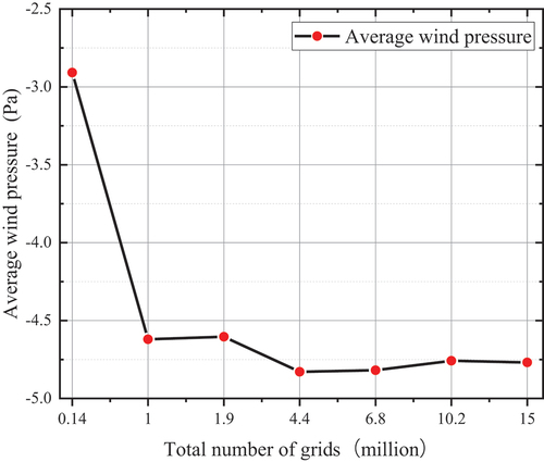
shows the average wind pressures of all roofs for the seven mesh densities. It can be observed that with an increase in grid density, the average wind pressure on the top surface of all blocks tends to be stable. When the total number of grids exceeds 4.4 million, the average wind pressure changed slightly. Considering the time cost, we selected a grid density of 0.0003 (total number of grids = 6.8 million) for the simulation.
Figure 4. Average wind pressure on roofs.
2.3. Comparison with wind tunnel data
2.3.1. Front and rear pressure differences in middle row
As shown in , the dimensionless coefficient of pressure difference (CPD) between the windward and leeward directions in the middle row of the 7 × 7 array was defined using EquationEquation (3)(3)
(3) (Buccolieri et al. Citation2019).
Figure 5. Middle column of a 7 × 7 matrix.
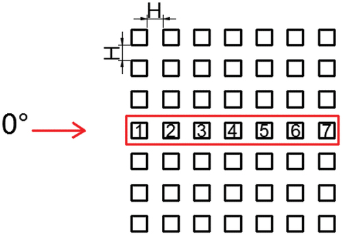
where and
represent the average pressures on the windward and leeward sides of the cube, respectively, and
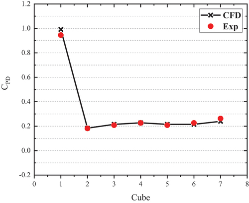
is the cube pressure difference of an isolated cube. The simulated and experimental values of CPD, which are very similar, are shown in .
Figure 6. Dimensionless pressure difference between windward and leeward sides.
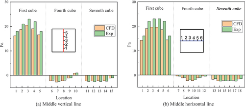
2.3.2. Pressure distribution on cubes
In this section, we further analyze the accuracy of wind pressure on the windward side of the 1st, 4th, and 7th cubes in the middle column of . shows the wind pressure along the vertical central line of the three cubes. The average error between the CFD simulation and wind tunnel experimental data (Buccolieri et al. Citation2019) was 11%. shows the wind pressure along the horizontal central line with an average error of 15%. The error of the two-line line mainly originates from the first cube, and the simulated value is smaller than the experimental value. However, the changing trends of the two were similar, and this error did not affect the relativity of the results.
Figure 7. Comparison of wind pressure on windward facades of buildings. (a) Middle vertical line, (b) Middle horizontal line.
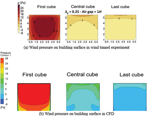
Meanwhile, the wind pressure distribution on the building surface of the 1st, 4th, and 7th cubes in the middle column were compared with the wind tunnel experimental results (Buccolieri et al. Citation2019). As shown in , it can be seen to be very similar.
Figure 8. Comparison of building surface wind pressure of buildings. (a) Wind pressure on building surface in wind tunnel experiment, (b) Wind pressure on building surface in CFD.
2.4. Potential assessment method based on standard deviation of wind pressure
In previous studies, the pressure difference between two facades was used to evaluate the wind pressure VP, as reported by Buccolieri et al. (Citation2019) But during the building design process, the architects want to have openings on the various facades for ventilation without restrictions. Therefore, this study proposes to measure the wind-ventilation potential of the building based on the pressure difference of the four facades on the cube.
2.4.1. Definition of ventilation potential based on standard deviation of wind pressure
In CFD software, such as Ansys fluent, the four sides of each block need to be defined separately. When outputting data after simulation, you need to select the output one by one separately, and then perform pressure data processing. When the number of models is too large, these steps will be cumbersome. A new evaluation method for ventilation potential is proposed. It only needs to set all four facades of the model as a whole, and the pressure data can be directly output after the simulation. The data processing steps are reduced, which is suitable for the situation of a large number of simulation models. Therefore, in this study, we intend to use the wind pressure standard deviation of all the facades to evaluate the natural VP. Specifically, the wind pressure ventilation capacity is discussed based on the nonuniformity of the outer surface of the building. The standard deviation of the wind pressure for each building, Pσ (Pa), is shown in Equation (4) (Ansys, Inc. Citation2021).
Where N is the pressure point on the surface, the number of pressure points is controlled by the number of grids divided, and the specific value location is explained in Section 30.3.1.17 of ANSYS Fluent-Theory Guide-Release 2021R1. Pi is the wind pressure (Pa) at position i, and is the average value of all points. ANSYS Fluent can directly calculate the standard deviation of the wind pressure on specified surfaces, which is very convenient for calculating the VP of buildings with any shape.
2.4.2. Comparison with “average pressure difference”
In the study of Tsutsumi, Katayama, and Nishida (Citation1992), the “average value of wind pressure coefficient difference” was used to evaluate the ventilation potential of the building. If four facades are considered, their method approximates Equationequation (5)(5)
(5) .
In which, is the average wind pressure,
the wind pressure difference(
) between the windward side and the leeward side,
the
between the windward side and the left side,
the
between the windward side and the right side,
the
between the left side and the right side,
the
between the left side and the leeward side,
the
between the right and leeward sides. In the 3 × 3, 5 × 5, and 7 × 7 arrays, their “wind pressure difference
” versus our “wind pressure standard deviation(Pσ)” is shown in .
Figure 9. “Wind pressure difference()” VS “Wind pressure standard deviation(Pσ)”.
Obviously our “wind pressure standard deviation(Pσ)” is proportional to the “wind pressure difference ”. For further proof, we took the 3 × 3, 5 × 5 and 7 × 7 arrays as the object, and explored the three wind directions of 0°, 22.5° and 45°. shows the correlation between the two ventilation potential evaluation methods: “wind pressure difference
” and “wind pressure standard deviation(Pσ)”. Their correlation coefficient r is EquationEquation (6)
(6)
(6) .
Table 1. Correlation coefficient r between “wind pressure difference()” and “wind pressure standard deviation(Pσ)” in different wind directions.
Where r is the correlation coefficient, is the average wind pressure of the i building in the building group,
is the average value of the average wind pressure of all buildings,
is the standard deviation of wind pressure for i building.
is the average of wind pressure standard deviations for all buildings.
It can be seen from that in different wind directions, the two ventilation potential evaluation methods of “wind pressure difference()” and “wind pressure standard deviation(Pσ)” have very good correlations. The lower correlation coefficients are all above 0.95. The variation trend of the “wind pressure standard deviation (Pσ)” ventilation potential evaluation method is very close to that of the “wind pressure difference
”. Therefore, in the block building model, it is reliable to use the “wind pressure standard deviation” to initially evaluate the ventilation potential of the building array.
Therefore in the next section, the standard deviation of the wind pressure on the four facades is taken as the wind VP of the building, which is referred to as the VP. Building density, alignment, lift, and meteorological data were analyzed for their impact on the VP.
3. Result analysis
3.1. Influence of building density
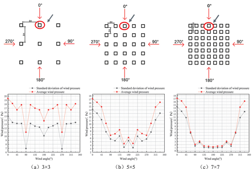
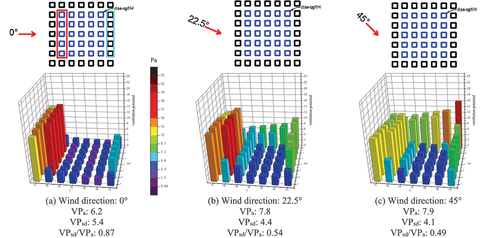
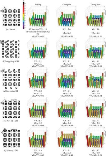
The building arrays are concentrated in an area of 13 H × 13 H, and four uniform densities of 3 × 3, 5 × 5, 7 × 7, and 9 × 9 are discussed. The spacing parameters are listed in , and the respective VPs are shown in . The average VP (VPa),the standard deviation of the VP (VPsd), and ratio of the second data point to the first data point, is the relative inhomogeneity of the VP value of each building are shown below each figure. The larger the VPsd/VPa value, more uneven is the VP. The average VP (VPa) and the standard deviation of the VP (VPsd) are calculated in EquationEquations (7)(7)
(7) and (Equation8
(8)
(8) ).
Figure 10. VP and uniformity of a 3 × 3 building array.
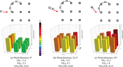
Figure 11. VP and uniformity of a 5 × 5 building array.
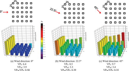
Figure 12. VP and uniformity of a 7 × 7 building array.
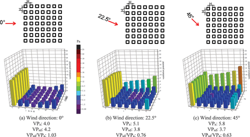
Figure 13. VP and uniformity of a 9 × 9 building array.
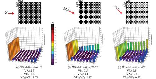
Table 2. Building density and spacing.
Where n is the number of all buildings. Pσ (Pa) is the standard deviation value of wind pressure, which is also the value of natural ventilation potential, see EquationEquation (4)(4)
(4) .
As shown in (3 × 3, 5 H spacing), for the 0° wind direction, the VP of the first row on the windward side is 1.5 times greater than that of the second row. However, the VP of all buildings was similar when the wind directions were 22.5° and 45°.
As shown in (5 × 5, 2 H spacing), when the wind direction is 0°, the VP of the first row of buildings on the windward side is 3.1 times larger than that of the second row. When the wind direction is 22.5°, the ratio of the first row to the second row on the windward side is 1.7. When the wind direction is 45°, the ratio of the first row to the second row is 1.4. However, VP of the first row is reduced by a factor of 0.93 times when the wind direction is 0°.
As shown in (7 × 7, 1 H spacing), for the 0° wind direction, VP of the first row is 5.3 times larger than that of the second row. When the wind direction is 22.5°, the ratio of the first row to the second row is 3.6. Simultaneously, the VP of the first row of buildings is 0.96 times of that when the wind direction is 0°. When the wind direction is 45°, the ratio of the first row to the second row is 2.6. Moreover, the VP of the first row of buildings is 0.84 times of that when the wind direction is 0°.
As shown in (9 × 9, 0.5 H spacing), for the 0° wind direction, the VP of the first row of buildings is 13.7 times larger than that of the second row. When the wind direction is 22.5°, the ratio of the first row to the second row is 7.7. Additionally, the VP of the first row of buildings is 0.93 times of that when the wind direction is 0°. When the wind direction is 45°, the ratio of the first row to the second row was 4.4, and the VP of the first row of buildings was 0.75 times of that when the wind direction is 0°.
It can be observed that when the density of the building group increases, the difference in VP between the front and rear rows is greater. When the wind direction changes to a certain angle, the difference in the building VP will be smaller. Simultaneously, VP in the first row decreases slightly.
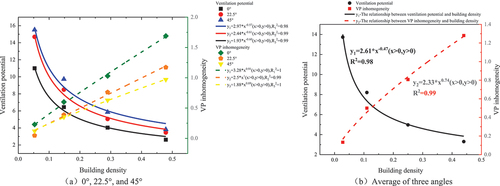
Because VP cannot be 0, nor can the building density be 0; a power function was used to fit the building density to the VPa, as shown in . Obviously, the trends for the three angles in (a) are similar, and their average curve is shown in (b). The two formulas (average of three angles) can be used to estimate the VPa in building planning.
Figure 14. Building density, VP, and VP inhomogeneity.
3.2. Staggered VS normal arrangement
In this section, we use a 7 × 7 array to analyze the effect of the staggered arrangement. The staggered arrangement was further divided into 0.5 times the H spacing () and 1 times the H spacing ().
Figure 15. Staggered arrangement, 7 × 7 array, 0.5H spacing.
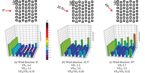
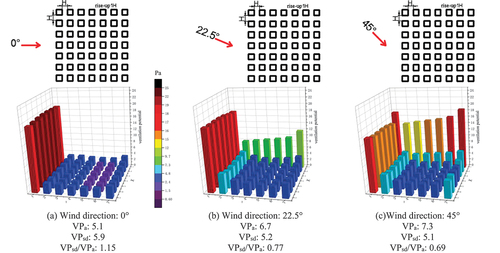
Figure 16. Staggered arrangement, 7 × 7 array, 1H spacing.
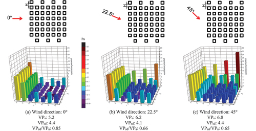
Compared with (normal alignment), VP of staggered 0.5 H and 1 H increased by 3% and 22%, whereas VPa/VPsd decreased by 23% and 11%, respectively. The uniformity of the VP increased after the staggering.
When the wind direction is 0°, as shown in (staggered 0.5 H) and (staggered 1 H), VP of the first row of buildings is 1.8 and 1.5 times larger than that of the second row, respectively. This is much smaller than that observed in (normal alignment) by a factor of 5.3. The building VP of the first row is 3.6 and 3.4 times larger than that of the third row. This is much smaller than that observed in (normal alignment) by a factor of 6.1. The first row is 6.2 and 5.1 times larger than the fourth row, respectively, which is slightly smaller than that observed in (normal alignment) by 7.1 times. The results for 22.5° and 45° wind directions were also similar. It can be observed that the staggered arrangement has an obvious improvement effect on the first three rows. Moreover, after staggering, the two columns of buildings in the edge area improved by approximately 2 times.
Overall, staggering can slightly improve the natural VP of the building array with an increase in uniformity.
3.3. Overall rise-up
In this section, we consider the effects of increasing the height by 1/3 H, 2/3 H, and 1 H, as shown in .
Figure 17. Rise-up 1/3H.
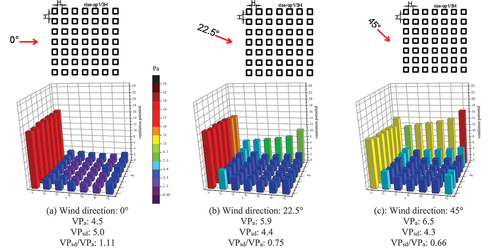
Figure 18. Overall rise-up 2/3H.
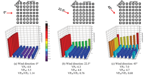
Figure 19. Overall rise-up 1H.
As observed from (rise-up 1/3 H), 18 (rise-up 2/3 H), and 19 (rise-up 1 H), compared with (no overhead), VP of the first row increased by 18%, 29%, and 39%, respectively. VP of the second line and the following lines are essentially unchanged. VPa of the building complex increased by 13%, 20%, and 28%, respectively. However, the nonuniformity (VPa/VPsd) increased by 8%, 11%, and 12%, respectively.
It can be observed that the overall rise-up only enhances the ventilation of the first row, but the improvement in the rear VP is small. Specifically, the distribution of the natural VP of the building array becomes more uneven.
3.4. Rise-up central area
As shown in Section Overall rise-up, the overall rise-up did not improve the natural VP of the rear buildings. Therefore, in this section, we attempt to overpass the central area of the building group. Additionally, we consider the intermediate 3 × 3 rise-up area with 1 H and intermediate 5 × 5 rise-up area with 1 H.
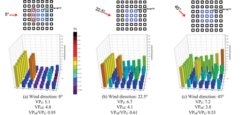
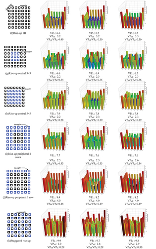
Comparing the information shown in (normal alignment; no overhead) and (3 × 3 area in the middle of the overhead), VPa of the building complex increases by 28% at 0° wind direction. VP of the three buildings surrounded by the orange line is 7 times that of the unsettled building. However, the VP increased by 63% for the three buildings enclosed by the light blue line. Simultaneously, VP in the middle 3 × 3 region increased by 242%. Second, the inhomogeneity of the VPa/VPsd ratio decreased by 8%. Similarly, VPa increased by 31% and 24% for 25° and 45° wind directions, respectively, and the inhomogeneous VPa/VPsd decreased by 20% and 16%, respectively.
Figure 20. Central 3 × 3 rise-up in a 7 × 7 array.
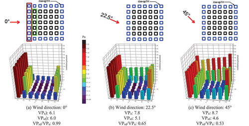
Similarly, as shown in (5 × 5 area in the middle of the overhead), VPa increased by 55%, 53%, and 36% for the three wind directions of 0°, 22.5°, and 45°, respectively. The nonuniformity (VPa/VPsd) decreased by 15%, 29%, and 22%, respectively.
Figure 21. Central 5 × 5 rise-up in a 7 × 7 array.
It can be observed that the overhead intermediate area can significantly improve the natural VP of the building array, and the effect of the 5 × 5 overhead center area is similar to that of the 3 × 3 overhead center area.
3.5. Rise-up peripheral area
In this section, we analyze the effect of the peripheral building overhead, including raising the outer two circles of the buildings () or raising the outer 1 circle of buildings ().
Figure 22. Peripheral 2 row rise-up by 1H in 7 × 7 array.
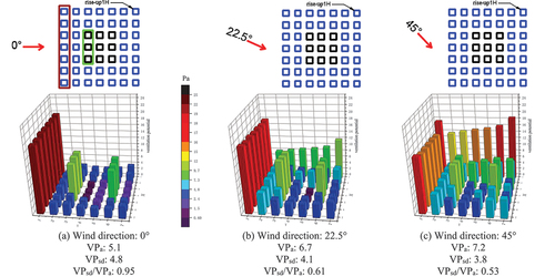
Figure 23. Peripheral 1 row rise-up by 1H in 7 × 7 array.
Compared with the information shown in (normal alignment; no rise-up), VPa of the building increases by an average of 28% for the 0° wind direction in . Among them, VP of the seven buildings enclosed by the brown line is 1.4 times that of the unraised building. VP of the three buildings surrounded by the green line is five times the VP of the unraised buildings. However, VP of the unraised buildings in the middle increased by 140%.
Relative to the normal arrangement (no rise-up) shown in , VP of the building shown in increased by 53% when the wind direction was 0°. VP of the seven buildings enclosed by the brown line is 1.4 times that of the unraised buildings. VP of the five buildings enclosed by the green line is 4.9 times that of the non-overhead building. However, VP of the unraised buildings in the middle increased by 78%.
Compared with the rise-up middle area, VP of the model shown in increased by 20%, and that shown in increased by 7%. The cases at 22.5° and 45° were similar.
It can be observed that compared with the rise-up central area (Section Rise-up central area), VP of the peripheral buildings increased and that of the central buildings decreased, i.e., the non-uniformity increased.
3.6. Staggered rise-up
Based on the conclusions mentioned in Sections Rise-up central area and Rise-up peripheral area, we realized that building overhead does improve natural ventilation, but the non-uniformity of VP is very obvious. Therefore, in this section, we propose a new staggered rise-up arrangement to study its effect on building arrays.
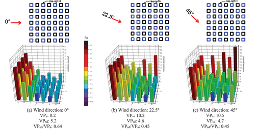
As shown in , compared to (normal alignment; no rise-up), VPa of the building complex increased by 95% for the three wind directions. Simultaneously, VP inhomogeneity (VPa/VPsd) decreased by an average of 36%. It can be observed that the staggered rise-up can significantly increase the VP and uniformity.
Figure 24. Staggered rise-up.
3.7. Annual frequency of wind direction
The results obtained in the previous sections show that wind direction can significantly affect the VP distribution of a building array. In this section, we considered the frequency of wind distribution in three cities in China to observe the magnitude of the VP throughout the year.
Three cities and their corresponding climate zones were selected: Beijing (cold climate zone), Changsha (hot summer and cold winter climate zone), and Guangzhou (hot summer and warm winter climate zones). Wind direction data were obtained from the Chinese Meteorological Dataset. (Department of Building Technology and Science, Tsinghua University Citation2005) A temperature suitable for natural ventilation (15–30 °C) was selected from a typical meteorological year, and the number of hours in the 16 wind directions was counted in the typical year. A wind rose diagram (frequency of wind direction) was drawn, as shown in , and VP throughout the year for different arrangements is shown in . Note that because of the similarity in airflow motion between buildings (Reynolds independence), the wind speed was not considered.
Figure 25. Wind-direction frequency in Beijing, Changsha, and Guangzhou.
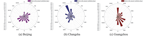
Figure 26. Annual VPa of Beijing, Changsha, and Guangzhou under different arrangements.
As shown in , although the wind direction frequencies in the three cities were significantly different, the VPs were almost the same. Hence, only Beijing is discussed below. The difference in the mean VP between (a) normal and (b) staggering 0.5 H is small, with the former being 20% more inhomogeneous than the latter. (c) The VP of staggering 1 H was 20% higher than that of the previous two. The potentials of (d) rise-up 1/3 H, (e) rise-up 2/3 H, and (f) rise-up 1 H increase in turn with similar inhomogeneities. VPa of (g) central 3 × 3 rise-up and (h) central 5 × 5 rise-up increased while the inhomogeneity decreased. The average potential of (i) peripheral two row rise-up and (j) peripheral one row rise-up increased, but the heterogeneity also increased. (k) The staggered rise-up had the largest increase in VP and the lowest inhomogeneity.
Figure 26. (Continued).
In summary, rise-up central and staggered rise-up are the best for wind VP.
3.8. Correlation between air age and potential distribution
Air age was first proposed by Sandberg et al. (Sandberg and Sjöberg Citation1983) in the 1980s and is defined as the time it takes for air to reach a certain position in the space from the inlet. This can reflect the freshness of indoor air. The smaller the air age, fresher the air and better the air quality. The tensor expression of the air age transport equation under steady-state conditions (Zhu Citation2016) is given using EquationEquation (9)(9)
(9) .
where τ is the air age at a certain point in the room; ρ is the air density; u is the velocity vector; is the diffusion coefficient of the air age;
; μ is the aerodynamic viscosity;
is the air turbulent viscosity;
and
are the Schmidt and turbulent Schmidt numbers, respectively. In this study, inlet of the flow field was used as the starting surface for calculation, and the above mentioned control equation of air age was compiled into a UDF(User defined function) to obtain the air age distribution.
To compare the correlation between air age distribution and the distribution of natural VP, the simulation results of a 7 × 7 normal arrangement and staggered overhead arrays matrix at three wind direction angles were used for comparison. The air age at a distance of 0.5 H m from the ground, which is at the horizontal plane of 0.0075 m. Based on the fact that windows can be opened all around the building, in order to assess the freshness of air around the building, the air-age value of a single building was obtained by averaging the air-age values of one point at each of the four azimuths of the building at 0.5 H. The value points are shown in , and the calculation formula is given in EquationEquation (10)(10)
(10) . The formula for calculating the standard deviation of air age is shown in EquationEquation (11)
(11)
(11) . The comparison between the distribution of natural VP and distribution of air age is shown in .
Figure 27. Locations of air age for Building a.
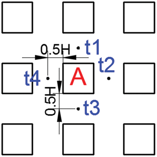
Figure 28. Distribution of air age in a 7 × 7 building array.
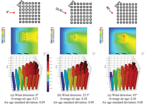
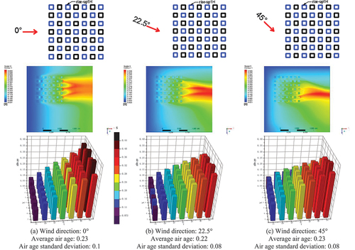
Figure 29. Distribution of air age in a Staggered rise-up building array.
where n is the number of squares in the computational array; is the air age value of the ith square, s; and
indicates the average air age value of all squares.
As shown in , in contrast to (normal alignment) for VP distribution, the distribution of the air age is opposite to the distribution of VP for the three wind directions. On the windward side, the air age was small, VP was high, and air quality was excellent. Conversely, downstream buildings had older air quality, low VP, and poor air quality. For a more special building arrangement with staggered overhead as shown in , the same conclusion can be obtained by comparing with the ventilation potential distribution in .
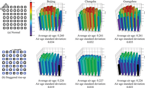
Compared with the staggered overhead in , in the three wind directions, the average air age of the buildings with the staggered overhead is smaller than that of the buildings with the positive arrangement. As mentioned in Section Staggered rise-up, the average ventilation potential of staggered overhead buildings is higher than that of positive arrangement, which can also confirm that the distribution of air age and building ventilation potential is in an opposite trend. Furthermore, after considering the distribution frequency of the wind direction throughout the year, the annual distribution of air age in the three typical climate regions of Beijing, Changsha, and Guangzhou is shown in . Compared with the information shown in (VP distribution), it can be observed that the distribution of natural ventilation potential has an opposite trend to the distribution of air age. In the dominant wind direction suitable for natural ventilation, the building on the windward side demonstrated smaller air age and better air quality. However, this advantage is not evident.
Figure 30. Annual distribution of air age in Beijing, Changsha, and Guangzhou climate zones.
4. Discussion
In this study, we discuss the effects of density, staggering, and lifting on natural ventilation using the standard deviation of wind pressure on building facades in ideal building arrays. The annual wind direction and wind distribution frequency were also considered.
It can be seen from sections Influence of building density, Staggered VS normal arrangement, Overall rise-up, Rise-up central area, Rise-up peripheral area, and Staggered rise-up that the incoming wind direction has a significant impact on the overall ventilation potential of the building complex. However, if the frequency of wind direction throughout the year is considered, the effect of wind direction is not obvious, as shown in Section Annual frequency of wind direction. This actually means that the orientation of the building complex has not much effect on the ventilation potential.
It can be found that the partial overhead (sections Rise-up central area and Rise-up peripheral area) and the staggered overhead (section Staggered rise-up) have better ventilation effects. The reason is that the distance between the buildings is widened and the density is reduced. This once again proves that density is the main factor affecting the ventilation potential of a building complex.
Similar to the experimental results obtained by Kim, Yoshida, and Tamura (Citation2012) and Buccolieri et al. (Citation2019) in a wind tunnel, we observed that the building density has a strong effect on the natural VP. The greater the building density, more uneven the VP distribution. Asfour (Citation2010) observed that when a building faces the dominant wind direction of the region, the VP of the building on the windward side is better, which is similar to the results obtained in this study. Citation2018) also suggested that the mainstream wind direction should be considered in a building row. However, in this study, we observed that the influence of mainstream wind direction became very small after considering the annual wind direction data.
Zhang, Gao, and Zhang (Citation2005) observed that a staggered layout could improve the ventilation effect of a building array. In this study, we found that the staggered layout only improved the ventilation in the first 2 or 3 rows of buildings, and the improvement of the overall ventilation effect of the building group is not obvious. It can be observed that the staggered arrangement has limitations in terms of the improvement effect of the wind environment. Hanna et al. (Citation2002) observed that the air velocity between buildings was nearly constant after the third row of an 8-row building array. In Zaki, Hagishima, and Tanimoto (Citation2012), it is mentioned that the pressure coefficients for a building density of 7.7% are diamond, square, and staggered, and the pressure coefficients for a
of 30.9%-39.1% are very similar regardless of the building arrangement. In this study, a
of 25% was used, and the difference in ventilation potential was found to be small when comparing square and staggered arrangements. Building density does have an effect on the ventilation potential for different building arrangements, and this paper is limited by considering only a building density of 25%. We will correct and further investigate this in our subsequent studies.
Tsutsumi, Katayama, and Nishida (Citation1992) observed that in an array with more than 10 rows, the wind pressure coefficient reached a stable value in the fifth row when the array was positive. However, when staggered, stable values were achieved in the seventh row. The standard deviation of wind pressure obtained in this study was almost unchanged after 2–3 rows. It can be seen that in a building array, after a certain number of rows, the wind speed and pressure do not change significantly.
Overall, in this study, we observed that building density has a significant impact on the natural ventilation potential of the building itself. The advantage of staggered alignment over normal alignment is not obvious when considering the frequency of wind direction throughout the year. A staggering rise-up can significantly increase VP and uniformity. The distribution of natural ventilation potential based on the wind pressure standards of the building facade shows an opposite trend to the air age distribution. But the method in the study are focusing on air change ability of each building in a layout, and the air age reflects the freshness of the outdoor air. They are related but have completely different meanings.
This study has several limitations. The shape of the building was too simplified (all considered as cubes), and factors, such as thermal buoyancy, pollutants, and terrain, were not considered. Also, many other arrays are not discussed.
5. Conclusion
The effects of different wind direction angles, different building densities, staggering, overall overhead, partial overhead, and wind direction frequency on the natural VP in the building array were simulated using CFD, and the conclusions are summarized as follows:
An evaluation method based on the standard deviation of wind pressure on the surface of the building can be used to evaluate the natural ventilation effect of the building group. It reveals the ventilation capacity of each building and is related to the air age, but its meaning is completely different. The air age reflects the freshness of the air.
The greater the density of the building group, smaller the potential, and this relationship behaves like an exponential function.
In a single wind direction, a staggered arrangement can improve VP. However, when considering the frequency of wind direction throughout the year, the effect becomes weak.
Raising the central area can improve the VP of an entire building array.
When the peripheral area is elevated, it will increase VP inhomogeneity between peripheral and intermediate area.
The staggered rise-up has a significant improvement effect on VP of the building group because the distance between the buildings is widened and the building density is reduced.
The assessing method and conclusions can be used for the planning and design of building locations in early stage. In the next study, the height and porosity of buildings will be discussed.
Acknowledgements
The original idea for the study originated from a collaboration with IEA-Annex62 Ventilative Cooling and IEA-Annex 80 Resilient Cooling.
Disclosure statement
No potential conflict of interest was reported by the authors.
Additional information
Funding
Notes on contributors
Zhong Yawen
Zhong Yawen currently is a master student in building envrionment and energy. She is now focusing on building natural ventilation and CFD simulation.
Yin Wei
Yin Wei serves as an associate professor of building envrionment and energy. His main research areas include natural ventilation, building wind environment, underground ventilation, subway station ventilation, kitchen ventilation, and ward ventilation in hospitals. On the other hand, he is currently moving towards passive houses and near-zero energy buildings.
Li Yonghan
Li Yonghan is a master student focusing on ventilative cooling. Hao Xiaoli Hao Xiaoli is a full professor in building envrionment and energy, who studies passive cooling techniques in buildings.
Zhang Shaobo
Zhang Shaobo is a PhD in cooling technology.
Han Qiaoyun
Han Qiaoyun is a PhD in ventilation of underground spaces.
Duan Shuangping
Duan Shuangping is an associate professor focusing on ventilative cooling and solar energy.
References
- Al-Sallal, K. A., M. M. AboulNaga, and A. M. Alteraifi. 2001. “Impact of Urban Spaces and Building Height on Airflow Distribution: Wind Tunnel Testing of an Urban Setting Prototype in Abu-Dhabi City.” Architectural Science Review 44 (3): 227–232. doi:10.1080/00038628.2001.9697477.
- Ansys, Inc. 2021. ANSYS Fluent-Theory Guide-Release 2021R1.
- Arkon, C. A., and Ü. Özkol. 2014. “Effect of Urban Geometry on Pedestrian-Level Wind Velocity.” Architectural Science Review 57 (1): 4–19. doi:10.1080/00038628.2013.835709.
- Asfour, O. S. 2010. “Prediction of Wind Environment in Different Grouping Patterns of Housing Blocks.” Energy and Buildings 42 (11): 2061–2069. doi:10.1016/j.enbuild.2010.06.015.
- Blocken, B., T. Stathopoulos, and J. Carmeliet. 2007. “CFD Simulation of the Atmospheric Boundary Layer: Wall Function Problems.” Atmospheric Environment 41 (2): 238–252. doi:10.1016/j.atmosenv.2006.08.019.
- Buccolieri, R., M. Sandberg, H. Wigö, and S. Di Sabatino. 2019. “The Drag Force Distribution Within Regular Arrays of Cubes and Its Relation to Cross Ventilation–Theoretical and Experimental Analyses.” Journal of Wind Engineering and Industrial Aerodynamics 189: 91–103. doi:10.1016/j.jweia.2019.03.022.
- Chand, I., P. K. Bhargava, and N. L. V. Krishak. 1998. “Effect of Balconies on Ventilation Inducing Aeromotive Force on Low-Rise Buildings.” Building and Environment 33 (6): 385–396. doi:10.1016/S0360-1323(97)00054-1.
- Dai, Y. W., C. M. Mak, and Z. T. Ai. 2019. “Computational Fluid Dynamics Simulation of Wind-Driven Inter-Unit Dispersion Around Multi-Storey Buildings: Upstream Building Effect.” Indoor and Built Environment 28 (2): 217–234. doi:10.1177/1420326X17745943.
- Department of Building Technology and Science, Tsinghua University. 2005. Meteorological Information Center of China Meteorological Administration Meteorological Data Set for Building Thermal Environment Analysis in China. Beijing, China: China Architecture & Building Press.
- Derakhshan, S., and A. Shaker. 2017. “Numerical Study of the Cross-Ventilation of an Isolated Building with Different Opening Aspect Ratios and Locations for Various Wind Directions.” International Journal of Ventilation 16 (1): 42–60. doi:10.1080/14733315.2016.1252146.
- Franke, J., A. Hellsten, K. H. Schlünzen, and B. Carissimo 2007. Best Practice Guideline for the CFD Simulation of Flows in the Urban Environment-A Summary. In 11th Conference on Harmonisation within Atmospheric Dispersion Modelling for Regulatory Purposes, Cambridge, UK, July 2007. Cambridge Environmental Research Consultants.
- Hang, J., and Y. Li. 2010. “Wind Conditions in Idealized Building Clusters: Macroscopic Simulations Using a Porous Turbulence Model.” Boundary-Layer Meteorology 136 (1): 129–159. doi:10.1007/s10546-010-9490-3.
- Hang, J., Y. Li, and M. Sandberg. 2011. “Experimental and Numerical Studies of Flows Through and Within High-Rise Building Arrays and Their Link to Ventilation Strategy.” Journal of Wind Engineering and Industrial Aerodynamics 99 (10): 1036–1055. doi:10.1016/j.jweia.2011.07.004.
- Hang, J., Z. Luo, M. Sandberg, and J. Gong. 2013. “Natural Ventilation Assessment in Typical Open and Semi-Open Urban Environments Under Various Wind Directions.” Building and Environment 70: 318–333. doi:10.1016/j.buildenv.2013.09.002.
- Hanna, S. R., S. Tehranian, B. Carissimo, R. W. Macdonald, and R. Lohner. 2002. “Comparisons of Model Simulations with Observations of Mean Flow and Turbulence Within Simple Obstacle Arrays.” Atmospheric Environment 36 (32): 5067–5079. doi:10.1016/S1352-2310(02)00566-6.
- Kim, Y. C., A. Yoshida, and Y. Tamura. 2012. “Characteristics of Surface Wind Pressures on Low-Rise Building Located Among Large Group of Surrounding Buildings.” Engineering Structures 35: 18–28. doi:10.1016/j.engstruct.2011.10.024.
- Kindangen, J., G. Krauss, and P. Depecker. 1997. “Effects of Roof Shapes on Wind-Induced Air Motion Inside Buildings.” Building and Environment 32 (1): 1–11. doi:10.1016/S0360-1323(96)00021-2.
- Lee, D. S., S. J. Kim, Y. H. Cho, and J. H. Jo. 2015. “Experimental Study for Wind Pressure Loss Rate Through Exterior Venetian Blind in Cross Ventilation.” Energy and Buildings 107: 123–130. doi:10.1016/j.enbuild.2015.08.018.
- Ling Chen, S., J. Lu, and W. W. Yu. 2017. “A Quantitative Method to Detect the Ventilation Paths in a Mountainous Urban City for Urban Planning: A Case Study in Guizhou, China.” Indoor and Built Environment 26 (3): 422–437. doi:10.1177/1420326X15626233.
- Liu, T., and W. L. Lee. 2019. “Using Response Surface Regression Method to Evaluate the Influence of Window Types on Ventilation Performance of Hong Kong Residential Buildings.” Building and Environment 154: 167–181. doi:10.1016/j.buildenv.2019.02.043.
- Mattsson, B. 2004. The Influence of Wind Speed, Terrain and Ventilation System on the Air Change Rate of a Single-Family House. In Thermal Sciences 2004. Proceedings of the ASME-ZSIS International Thermal Science Seminar II. Begel House Inc.
- Montazeri, H., and B. Blocken. 2013. “CFD Simulation of Wind-Induced Pressure Coefficients on Buildings with and Without Balconies: Validation and Sensitivity Analysis.” Building and Environment 60: 137–149. doi:10.1016/j.buildenv.2012.11.012.
- Ok, V., E. Yasa, and M. Özgunler. 2008. “An Experimental Study of the Effects of Surface Openings on Air Flow Caused by Wind in Courtyard Buildings.” Architectural Science Review 51 (3): 263–268. doi:10.3763/asre.2008.5131.
- Ricci, A., I. Kalkman, B. Blocken, M. Burlando, and M. P. Repetto. 2020. “Impact of Turbulence Models and Roughness Height in 3D Steady RANS Simulations of Wind Flow in an Urban Environment.” Building and Environment 171: 106617. doi:10.1016/j.buildenv.2019.106617.
- Sandberg, M., and M. Sjöberg. 1983. “The Use of Moments for Assessing Air Quality in Ventilated Rooms.” Building and Environment 18 (4): 181–197. doi:10.1016/0360-1323(83)90026-4.
- Shirzadi, M., M. Naghashzadegan, and P. A. Mirzaei. 2018. “Improving the CFD Modelling of Cross-Ventilation in Highly-Packed Urban Areas.” Sustainable Cities and Society 37: 451–465. doi:10.1016/j.scs.2017.11.020.
- Tominaga, Y., and B. Blocken. 2015. “Wind Tunnel Experiments on Cross-Ventilation Flow of a Generic Building with Contaminant Dispersion in Unsheltered and Sheltered Conditions.” Building and Environment 92: 452–461. doi:10.1016/j.buildenv.2015.05.026.
- Tominaga, Y., A. Mochida, T. Shirasawa, R. Yoshie, H. Kataoka, K. Harimoto, and T. Nozu. 2004. “Cross Comparisons of CFD Results of Wind Environment at Pedestrian Level Around a High-Rise Building and Within a Building Complex.” Journal of Asian Architecture and Building Engineering 3 (1): 63–70. doi:10.3130/jaabe.3.63.
- Tsutsumi, J., T. Katayama, and M. Nishida. 1992. “Wind Tunnel Tests of Wind Pressure on Regularly Aligned Buildings.” Journal of Wind Engineering and Industrial Aerodynamics 43 (1–3): 1799–1810. doi:10.1016/0167-6105(92)90592-X.
- van Hooff, T., and B. Blocken. 2013. “CFD Evaluation of Natural Ventilation of Indoor Environments by the Concentration Decay Method: CO2 Gas Dispersion from a Semi-Enclosed Stadium.” Building and Environment 61: 1–17. doi:10.1016/j.buildenv.2012.11.021.
- Van Hooff, T., and B. Blocken. 2020. “Mixing Ventilation Driven by Two Oppositely Located Supply Jets with a Time-Periodic Supply Velocity: A Numerical Analysis Using Computational Fluid Dynamics.” Indoor and Built Environment 29 (4): 603–620. doi:10.1177/1420326X19884667.
- van Hooff, T., B. Blocken, and Y. Tominaga. 2017. “On the Accuracy of CFD Simulations of Cross-Ventilation Flows for a Generic Isolated Building: Comparison of RANS, LES and Experiments.” Building and Environment 114: 148–165. doi:10.1016/j.buildenv.2016.12.019.
- Wang, W., and E. Ng. 2018. “Large-Eddy Simulations of Air Ventilation in Parametric Scenarios: Comparative Studies of Urban Form and Wind Direction.” Architectural Science Review 61 (4): 215–225. doi:10.1080/00038628.2018.1481359.
- Wang, T. W., W. Yin, L. L. Fu, and Z. Y. Zhang. 2022. “Estimation Model for Natural Ventilation by Wind Force Considering Wind Direction and Building Orientation for Low-Rise Building in China.” Indoor and Built Environment 31 (8): 2036–2052. doi:10.1177/1420326X20944983.
- Wei, Y., Z. Guo-Qiang, W. Xiao, L. Jing, and X. San-Xian. 2010. “Potential Model for Single-Sided Naturally Ventilated Buildings in China.” Solar Energy 84 (9): 1595–1600. doi:10.1016/j.solener.2010.06.011.
- Yin, W., G. Zhang, W. Yang, and X. Wang. 2010. “Natural Ventilation Potential Model Considering Solution Multiplicity, Window Opening Percentage, Air Velocity and Humidity in China.” Building and Environment 45 (2): 338–344. doi:10.1016/j.buildenv.2009.06.012.
- Zaki, S. A., A. Hagishima, and J. Tanimoto. 2012. “Experimental Study of Wind-Induced Ventilation in Urban Building of Cube Arrays with Various Layouts.” Journal of Wind Engineering and Industrial Aerodynamics 103: 31–40. doi:10.1016/j.jweia.2012.02.008.
- Zhang, A., C. Gao, and L. Zhang. 2005. “Numerical Simulation of the Wind Field Around Different Building Arrangements.” Journal of Wind Engineering and Industrial Aerodynamics 93 (12): 891–904. doi:10.1016/j.jweia.2005.09.001.
- Zhang, Z. Y., W. Yin, T. W. Wang, Y. H. Li, Y. W Zhong, and G. Q. Zhang. 2021. “Potential of Cross-Ventilation Channels in an Ideal Typical Apartment Building Predicted by CFD and Multi-Zone Airflow Model.” Journal of Building Engineering 44: 103408. doi:10.1016/j.jobe.2021.103408.
- Zhang, Z. Y., W. Yin, T. W. Wang, and A. O’donovan. 2022. “Effect of Cross-Ventilation Channel in Classrooms with Interior Corridor Estimated by Computational Fluid Dynamics.” Indoor and Built Environment 31 (4): 1047–1065. doi:10.1177/1420326X211054341.
- Zhen, M., D. Zhou, G. Bian, Y. Yang, and Y. Liu. 2019. “Wind Environment of Urban Residential Blocks: A Research Review.” Architectural Science Review 62 (1): 66–73. doi:10.1080/00038628.2018.1528967.
- Zhu, Y. X. 2016. Built Environment. 4th ed. Beijing, China: China Architecture & Building Press.