Three neural networks for prestressed fiber-reinforced polymer/plastics sheet-reinforced concrete beams

ABSTRACT

This paper introduces a method for predicting the flexural ultimate load of prestressed fiber-reinforced polymer/plastics sheet-reinforced concrete beams. The main work of this paper is as follows: three artificial neural network models of back propagation, Levenberg-Marquardt, and Bayesian Regularization predict the flexural ultimate loads of prestressed FRP-RC and were constructed using a database of 243 concrete beams from various previous studies. The optimal hidden layer node of the neural network is determined as 17 using MSE value, R-value and average error as evaluation metrics. The optimal value of each parameter in the neural network is determined using MSE value as metrics. A series of simulations showed that the Bayesian Regularization model with 17 nodes in the hidden layer best matches the experimental results with root mean square error and correlation coefficient (R) values of 0.002256 and 0.97972, respectively, and an average error of 8.79%. The contribution analysis of the input variables indicates that the flexural capacity of the RC beam was most significantly influenced by its width, elastic modulus, and lower reinforcement, with relative importance of 10.38%, 9.88%, and 9.56%, respectively. Noisy data in the input layer is eliminated using Singular Value Decomposition, optimizing the performance of neural networks.

KEYWORDS:

• Prestressed FRP sheet
• reinforced concrete
• flexural load capacity
• neural network
• contribution analysis

1. Introduction

Sheet reinforcement is one of the most effective means of increasing the load-carrying capacity of a structure by improving its compressive and flexural properties as well as providing effective seismic protection for the structure (Wang and Zhou 2023b). And since the 1990s, fiber-reinforced polymer/plastics (FRP) has been at the forefront of research. The FRP fiber material has many advantages, such as being lightweight, easy to construct, corrosion resistant, good durability, high strength-to-mass density ratio, and good fatigue performance, which is ideal for concrete structure reinforcement (Ye and Peng 2006). Compared with ordinary FRP reinforcement, bonded prestressed FRP can improve the reinforced concrete (RC) beam performance and ultimate load capacity by mitigating the problems of inadequate high-strength properties and stress hysteresis (Lu et al. 2006).

Flexural strength is an important basis for structural design and construction and is one of the most important concrete properties. The concrete quality is directly related to evaluating and accepting sub-projects, divisional works, and unit works. However, traditional experimental methods to measure the flexural strength of concrete, from sampling to conducting tests and analyzing the results, not only require considerable manpower and material resources but also require a long time. This makes it impossible to use the information most closely related to the current project in project management, which is unfavorable to speeding up construction progress and conserving construction funds and materials. Therefore, empirical prediction formulas have been used to meet the requirements of timely decisions during construction for many years. However, these formulas only consider certain quantitative factors for judgment, and some factors affecting the formula externally can only be generalized to their limits, resulting in the detection and calculation results that deviate wildly. The poor accuracy of traditional prediction methods makes it challenging to apply universally in practice. Scholars have studied the performance of structures through data analysis methods (Wang and Zhou 2023a). Therefore, this paper introduces an artificial neural network (ANN) to study prestressed FRP-RC beams.

The ANN is a nonlinear information processing tool that can learn from existing large data sets that may contain multiple predictors. Its ability to perform extensive mathematical mappings by recognizing patterns or classifying data, even with incomplete information, sets it apart from conventional problem-solving approaches. As the primary model for predicting flexural ultimate loads in RC, the ANN is a data-driven model with stronger capabilities to handle highly nonlinear and complex problems over other methods. For RC, the flexural ultimate load is influenced by various factors, such as material properties and geometric parameters. The ANN can effectively capture the complex relationships between these factors and has a strong capacity to adaptively adjust its weights and biases during training to improve the prediction accuracy. This adaptive learning capability allows ANNs to have better generalization performance and less overfitting than other traditional models.

A typical neural network topology includes an input layer that passes data to the hidden layers, performs computations, and transmits information to the output layer. Depending on the desired ANN architecture, the hidden layers or computation nodes consist of one or more layers (Nolan 2022). Numerous industries, including civil engineering, have seen a rise in neural network and machine learning (ML) studies in recent years. ML uses learning algorithms to uncover input and output links of complex nonlinear systems. Arash Teymori Gharah (Teymori Gharah Tapeh and Naser 2023) introduced standard algorithms and techniques of artificial intelligence (AI), ML, and deep learning for structural engineers. Akinosho and Oyedele (2020) performed a scientometric analysis of over 4,000 scholarly publications and structural health monitoring, damage detection, and structural material performance predictions collected from over 200 sources to identify best practices in terms of procedures, performance metrics, and dataset sizes as well as a review of past and recent efforts to apply AI derivatives to various subfields of structural engineering. Their results indicate that ANNs and genetic algorithms have the largest share of publications, occupying about 55.9%. Numerous common neural network architectures and their current applications in the construction sector were presented. They revealed how neural networks have been effectively used in construction with potential future applications with focus on any difficulties that may arise. Dogan and Birant (2021) briefly overviewed various types of ML techniques, examined current trends in manufacturing, discussed the special benefits of ML in the workplace, and pinpointed current applications along with the most effective methods for necessary tasks.

Researchers are now working on more precise and complex prediction models, which includes various hybrid models that consider time series. Yuan et al. (2018) investigated the accuracy of a hybrid long short-term memory neural network and ant lion optimizer model (LSTM-ALO) to predict monthly runoff. Scatter plots and box line plots evaluated the performance of other models with the LSTM-ALO, indicating the LSTM-ALO has a higher accuracy and provides an effective method for monthly runoff forecasting. Adnan et al. (2022) proposed a hybrid algorithm, ANFIS-GBO, to accurately estimate flow in a mountainous watershed. The GBO algorithm improves the prediction accuracy of ANFIS more than other benchmark methods. Adnan et al. (2021) proposed a hybrid model for predicting monthly runoff forecasts.Comparing the ELM-PSOGWO with ELM, ELM-PSO, ELM-GWO, and ELM-PSOGSA methods show that the ELM-PSOGWO method is more successful than the other benchmark models.

Ikram et al. (2022) accurately predicted renewable, environmentally friendly, and carbon-free energy resources. The improved version of the multiverse optimizer algorithm (IMVO) was utilized with the integration of the least square support vector machine for better tuning of the hyperparameters. Adnan et al. (2022) integrated the simulated annealing algorithm with the mayfly optimization algorithm (SAMOA) to determine the optimal hyperparameters for support vector regression (SVR) to overcome the exploration weakness of the mayfly optimization algorithm method and the hybrid SVR-SAMOA model to accurately predict water flow.

Ikram et al. (2022) developed the extended marine predator algorithm (EMPA)-based ANN (ANN-EMPA) as a novel hybridized ML method for streamflow estimation in the Upper Indus Basin, a key mountainous glacier melt-affected basin of Pakistan. In civil engineering, Ikram et al. (2022) utilized an Extreme Learning Machine network based on the Chaos Red Fox Optimization Algorithm (ELM-CRFOA) to predict the shear strength of RC beams with composite steel. The accuracy of the method was demonstrated by comparing model predictions with cumulative data and available shear design equations. A sensitivity analysis was performed to investigate the effects of input parameters on the shear strength of FRP-RC beams.

Many researchers have adopted ANN techniques in civil engineering to predict concrete mechanical performance (Mashhadban, Kutanaei, and Sayarinejad 2016; Cascardi, Micelli, and Aiello 2017; Congro 2021; Bhagwat and Nayak 2023; Li and Deng 2004; Ahmad 2020; Ashrafi 2010) used five ANNs with the Bayesian Regularization (BR) algorithm to predict the residual strength of fibrous concrete under bending loads. Predictions of the best neural networks well-matched test load results. Bhagwat et al. (2023) used three resilient back propagation (BP) neural networks to predict the flexural strength of corroded prestressed concrete beams. The proposed model converges before the other backpropagation algorithms. The height and span of the beam are important factors affecting the ultimate load, ultimate bending moment, and deflection, respectively. Li and Deng (2004) used test data and applied the principle of the BP neural networks to establish a model that predicts the flexural load capacity of steel fiber concrete beams reinforced with carbon fiber fabric.

Ahmad (2020) developed a framework for developing an ANN capable of realistically predicting the load-carrying capacity of RC members. Reza Ashrafi, Jalal, and Garmsiri (2010) used neural network techniques to predict load-displacement curves and the concrete compressive strength based on mixed proportions, all with satisfactory results. However, there is no prediction of the flexural performance of prestressed FRP-RC beams. Therefore, in order to be able to accurately predict the flexural ultimate load of prestressed FRP reinforced reinforced concrete beams for the design of concrete beams. In this paper, 243 sets of experimental data were collected and three ANNs, including traditional BP neural network, Levenberg-Marquardt (L-M) neural network and BR neural network, were used to predict the flexural ultimate load of prestressed FRP-RC beam.The effect of factors in the input layer on the flexural ultimate load of prestressed FRP-RC beam has been investigated.The details of the work are as follows:

• The optimal structure of the neural network model and optimal parameters are determined.

• Three neural network models are trained, and their performances are compared.

• Contributions of the input variables are analyzed to investigate the influence of the input variables on the output variable to comprehensively understand the prediction models.

• The noisy data in each model were eliminated using the singular value decomposition (SVD) method.

2. Experimental samples and evaluation index

2.1. Data sources and distribution

To accurately predict the ultimate flexural load capacity of prestressed FRP-RC, 243 sets of test data were collected from existing studies (Du 2005; Wang 2003; Li 2015; Zhou 2015; Tai 2018; Tian 2006; Lai 2016; Sun 2021; Chen 2009; Xiang 2015; Wu 2018; Ge 2006; Jiang 2008; Wang 2022; Wang and Zhou 2005; Fei and Jiang 2003; Shang 2003; Yang and Park 2008; Gao, Gu, and Mosallam 2016; Peng 2013; Garden and Hollaway 1997; Gaafar and El-Hacha 2008; You 2012; Wooa 2008; Mukherjee 2009) (see the attachment). The data were cited as real and valid and only normalized here. Then, 70% of the data (170 sets) were used for training and 30% (73 sets) were used for testing. The standard normalization formula is:

(1) $X_i=\frac{{X_i}^{\prime }-{{\mathit{X}}_{min}}^{\prime }}{{{\mathit{X}}_{max}}^{\prime }-{{\mathit{X}}_{min}}^{\prime }}$(1)

where${{\mathit{X}}_{max}}^{\prime },{{\mathit{X}}_{min}}^{\prime },{X_i}^{\prime }$ are the maximum, minimum, and measured values of the network input vectors in the original data, respectively. The difficulty of the ANN model and errors are both reduced after normalizing.

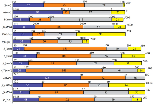
Thirteen influencing factors were chosen as the input layer of the neural network. These are the width (t_f), thickness (b_f), bond length (L), tensile strength (f_t), modulus of elasticity (E_f), prestress applied to FRP sheet (P_f), width and height of the RC beam section (b_c and h_c), upper reinforcement (A_s), lower reinforcement (A_s^(b)), modulus of elasticity (E), compressive strength of concrete (f_cu), tensile strength of concrete (f_u), etc. The only output for network model is the corresponding flexural ultimate load capacity of the strengthened RC beam (P_u). Figure 1 clearly illustrates the range of 13 input variables and 1 output variable. (Where the number on the histogram indicates the range in which the variable is located and the number within the histogram indicates the number of that variable within that range.)

Figure 1. Distribution of the input and output variables of the neural network.

2.2. Model evaluation metrics

Existing literature on the performance indexes indicate that the influence of the magnitude is eliminated (Botchkarev 2019; Naser 2021) in the neural networks due to data normalization. To avoid mutual offsets of positive and negative errors, four absolute value errors or squared errors, such as the mean absolute error (MAE), mean square error (MSE), correlation coefficient (R), and root mean square error are selected as the performance evaluation indexes of three neural networks. The R represents the degree of fit of the regression results to the measured values. A closer value to 1 means a better fit. The root mean square error and MSE values reflect the degree of difference between the predicted and measured values, with a smaller value indicating a greater model accuracy. To facilitate designers’ intuition with the prediction accuracy and neural network efficiency, the performance index mean absolute percentage error (MAPE) and comparisons of the CPU time consumed at the end of training the algorithm are added to visually evaluate the neural network. The specific required calculation formulas are:

(2) $\mathit{MAE}=\frac{1}{n}\sum _{\mathit{i}=1}^n\left|y_i-{y_i}^{\ast }\right|$(2)

(3) $\mathit{MSE}=\frac{1}{n}\sum _{\mathit{i}=1}^n(y_i-{y_i}^{\ast }{)}^2$(3)

(4) $\mathit{RMSE}=\sqrt{\frac{1}{n}\sum _{\mathit{i}=1}^n{(y_i-{y_i}^{\ast })}^2}$(4)

(5) $\mathit{R}=\frac{\sum _{\mathit{i}=1}^n((y_i-\bar{y})({y_i}^{\ast }-\overline{y^{\ast }}))}{\sqrt{\sum _{\mathit{i}=1}^n{(y_i-\bar{y})}^2\sum _{\mathit{i}=1}^n{({y_i}^{\ast }-\overline{y^{\ast }})}^2}}$(5)

(6) $\mathit{MAPE}=\frac{1}{n}\sum _{\mathrm{i}=1}^n\frac{y_i-{y_i}^{\ast }}{y_i}$(6)

where: $\mathit{Accessisdenied}$ denotes the number of samples $\mathit{y},\overline{y},y^{*}$, and $\overline{{\mathbf{y}}^{\ast }}$ represent the actual sample value, sample mean, model predicted value, and model predicted mean, respectively.

3. Three algorithms for ANNs

3.1. BP neural network

The BP neural network is a multilayer feedforward approach trained with the error BP algorithm, which is one of the most widely used models. The BP neural network learns and stores several input-output pattern mapping relationships without revealing the associated mathematical equations beforehand. Its learning rule uses gradient descent to continuously adjust the weights and thresholds of the network via BP to minimize the sum of squared network errors. The BP neural network model includes the input, hidden, and output layers.

3.2. L – M neural network

The L – M neural network achieves convergence characteristics by adaptively adjusting the damping factor. This approach has a higher iterative convergence speed and obtains stable and reliable solutions in many nonlinear optimization problems. The original BP learning algorithm uses gradient descent, and the parameters move opposite to the error gradient so that the error decreases until satisfying the requirement. The L – M algorithm is a combination of gradient descent and the Gauss – Newton method with both local convergence of Gauss – Newton and global characteristics of gradient descent. Its gradient descent is fast with fewer training steps than the traditional BP neural network. So, the L – M algorithm optimizes the BP algorithm (Wei Peng 2016). The following are some brief descriptions of the iterative approach of the L – M algorithm:

(7) ${\mathit{\omega }}^{\mathit{\kappa }+1}={\mathit{\omega }}^{\mathit{\kappa }}+\mathrm{\Delta \omega }$(7)

(8) $\mathrm{\Delta \omega }=[J^T(\mathit{\omega })\mathit{J}(\mathit{\omega })+\mathit{\mu I}{]}^{-1}{J}^T(\mathit{\omega })\mathit{e}(\mathit{\omega })$(8)

where $\mathit{\omega }$ denotes the network weights and thresholds, ${\omega }^k$ denotes the vector consisting of the weights and thresholds of the $\mathit{k}$th iteration, ${\omega }^{\mathit{k}+1}$ denotes the vector consisting of the new weights and thresholds, $\mathrm{\Delta \omega }$ denotes the weight increments, $\mathit{\mu }$ denotes the user-defined learning rate, $\mathit{I}$ denotes the unit matrix, $\mathit{e}(\mathit{\omega })$ denotes the error, and $\mathit{J}(\mathit{\omega })$ denotes the Jacobian matrix as:

(9) $\mathit{J}(\mathit{\omega })=\left|\begin{array}{c}\frac{\mathrm{\partial }{e}_1(\mathit{\omega })}{\mathrm{\partial }{\omega }_1}\cdot \cdot \cdot \cdot \cdot \cdot \cdot \frac{\mathrm{\partial }{e}_1(\mathit{\omega })}{\mathrm{\partial }{\omega }_n}\\ ⋮\ddots ⋮\\ \frac{\mathrm{\partial }{e}_N(\mathit{\omega })}{\mathrm{\partial }{\omega }_1}\cdot \cdot \cdot \cdot \cdot \cdot \cdot \frac{\mathrm{\partial }{e}_N(\mathit{\omega })}{\mathrm{\partial }{\omega }_n}\end{array}\begin{array}{c}\mathit{\hspace{0.17em}}\\ \mathit{\hspace{0.17em}}\\ \mathit{\hspace{0.17em}}\\ \mathit{\hspace{0.17em}}\\ \mathit{\hspace{0.17em}}\end{array}\right|$(9)

In practice, $\mathit{\mu }$ is a trial parameter. For a given $\mathit{\mu }$, if the resulting $\mathrm{\Delta \omega }$ decreases the error indicator function $\mathit{E}(\mathit{\omega })$, then $\mathit{\mu }$ decreases. Otherwise, $\mathit{\mu }$ increases. Therein, the error indicator function can be quickly reduced to its minimum value. The error indicator function is given by:

(10) $\mathit{E}(\mathit{\omega })=\frac{1}{2\mathit{P}}\sum \begin{array}{c}\mathit{P}\\ \mathit{i}=1\end{array}||Y_i-{Y_i}^{\prime }||{ }^2=\frac{1}{2\mathit{P}}\sum \begin{array}{c}\mathit{P}\\ \mathit{i}=1\end{array}{e_i}^2(\mathit{\omega })$(10)

where $Y_i$ denotes the desired network output vector, ${Y_i}^{\prime }$ denotes the actual output vector, and $\mathit{P}$ denotes the number of samples.

3.3. BR neural network

The BR neural network combines the traditional least squares error function with an additional regularization term. This gives the equation:

(11) $\mathit{S}(\mathit{w})=\mathit{\beta }{E}_D+\mathit{\alpha }{E}_W;E_W=\sum _{\mathit{i}=1}^m{w_i}^2$(11)

where the terms $\mathit{\alpha }$ and $\mathit{\beta }$ are regularization parameters or hyperparameters, $E_w$ is the penalty term for large weights, and $\mathit{m}$ is the number of weights. In the Bayesian framework, the learning process considers weight vector uncertainty by assigning a probability distribution representing the relative confidence for different values. The function is initially set to some prior distribution. Once the data are observed, they can be converted into a posterior distribution using Bayes’ theorem as:

(12) $\mathit{P}(\mathit{w}|\mathit{\alpha },\mathit{\beta },\mathit{D})=\frac{\mathit{P}(\mathit{D}\left|\mathit{w},\mathit{\beta })\mathit{P}(\mathit{w}\right|\alpha )}{\mathit{P}(\mathit{D}|\alpha ,\beta )}$(12)

where $\mathit{P}(\mathit{w}|\mathit{\alpha })$ is the prior density indicating the confidence level in the weights before any data are collected, $\mathit{P}(\mathit{D}|\mathit{w},\mathit{\beta })$ is the likelihood function giving the error probability, and $\mathit{P}(\mathit{D}|\mathit{w},\mathit{\beta })$ is the normalization factor also called the evidence of the model equation. Equation (11)(11) $\mathit{S}(\mathit{w})=\mathit{\beta }{E}_D+\mathit{\alpha }{E}_W;E_W=\sum _{\mathit{i}=1}^m{w_i}^2$(11) can be expressed in words as:

(13) $\mathit{Posterior}=\frac{\mathit{Likelihood}.\mathit{prior}}{\mathit{Evidence}}$(13)

The optimal weights of the model are obtained by maximizing the posterior probability during training. This corresponds to the regularized objective function with the minimization of Equation (10)(10) $\mathit{E}(\mathit{\omega })=\frac{1}{2\mathit{P}}\sum \begin{array}{c}\mathit{P}\\ \mathit{i}=1\end{array}||Y_i-{Y_i}^{\prime }||{ }^2=\frac{1}{2\mathit{P}}\sum \begin{array}{c}\mathit{P}\\ \mathit{i}=1\end{array}{e_i}^2(\mathit{\omega })$(10) . Assuming that the weights and data probability distribution are Gaussian, the prior probability of the weights can be written as:

(14) $\mathit{P}(\mathit{w}|\mathit{\alpha })=\frac{1}{Z_W(\mathit{\alpha })}exp(-\mathit{\alpha }{E}_W)$(14)

Similarly, the probability of the error can be written as:

(15) $\mathit{P}(\mathit{D}|\mathit{w},\mathit{\beta })=\frac{1}{Z_D(\mathit{\beta })}exp(-\mathit{\beta }{E}_D)$(15)

Then, the final posterior distribution can be obtained as:

(16) $\mathit{P}(\mathit{w}|\mathit{\alpha },\mathit{\beta },\mathit{D})=\frac{1}{Z_S(\mathit{\alpha },\mathit{\beta })}exp(-\mathit{S}(\mathit{w}))$(16)

For the regularization parameters $\mathit{\alpha }$ and $\mathit{\beta }$, we use Bayes’ theorem to infer the optimal value of the regularization parameter from the data.

(17) $\mathit{P}(\mathit{\alpha },\mathit{\beta }|\mathit{D})=\frac{\mathit{P}(\mathit{D}|\alpha ,\beta )P(\alpha ,\beta )}{\mathit{P}(\mathit{D})}$(17)

where $\mathit{P}(\mathit{\alpha },\mathit{\beta })$ is the prior probability of the regularization parameters $\mathit{\alpha }$ and $\mathit{\beta }$, $\mathit{P}(\mathit{D}|\mathit{\alpha },\mathit{\beta })$ is the likelihood term called the evidence for $\mathit{\alpha }$ and $\mathit{\beta }$, where $\mathit{\alpha }$ is the optimal value obtained based on Equation (11)(11) $\mathit{S}(\mathit{w})=\mathit{\beta }{E}_D+\mathit{\alpha }{E}_W;E_W=\sum _{\mathit{i}=1}^m{w_i}^2$(11) . The effective parameters are given by:

(18) $\mathit{\alpha }=\mathit{\gamma }/2E_W;\mathit{\beta }=\left(\mathit{n}-\mathit{\gamma }\right)/2E_D;\mathit{\gamma }=\sum _{\mathit{i}=1}^m\mathit{m}-\mathit{\alpha }.\mathit{trac}{e}^{-1}\left(\mathit{A}\right)$(18)

where $\mathit{m}$ is the number of parameters, and $\mathit{A}$ is the Hessian matrix of the objective function $\mathit{S}(\mathit{w})$.

In the Bayesian framework, an optimization process finds the optimal weights in Equation (10)(10) $\mathit{E}(\mathit{\omega })=\frac{1}{2\mathit{P}}\sum \begin{array}{c}\mathit{P}\\ \mathit{i}=1\end{array}||Y_i-{Y_i}^{\prime }||{ }^2=\frac{1}{2\mathit{P}}\sum \begin{array}{c}\mathit{P}\\ \mathit{i}=1\end{array}{e_i}^2(\mathit{\omega })$(10) and the optimal values of in Equation (16)(16) $\mathit{P}(\mathit{w}|\mathit{\alpha },\mathit{\beta },\mathit{D})=\frac{1}{Z_S(\mathit{\alpha },\mathit{\beta })}exp(-\mathit{S}(\mathit{w}))$(16) . The iterative process is given as follows.

1. Select the initial values and weights for $\mathit{\alpha }$ and $\mathit{\beta }$.

2. Adopt the L – M algorithm to find the weights that minimize the objective function in Equation (5)(5) $\mathit{R}=\frac{\sum _{\mathit{i}=1}^n((y_i-\bar{y})({y_i}^{\ast }-\overline{y^{\ast }}))}{\sqrt{\sum _{\mathit{i}=1}^n{(y_i-\bar{y})}^2\sum _{\mathit{i}=1}^n{({y_i}^{\ast }-\overline{y^{\ast }})}^2}}$(5) .

3. Calculate the valid number of parameters $\mathit{\gamma }$ and the new values of $\mathit{\alpha }$ and $\mathit{\beta }$.

4. Repeat steps (2) and (3) until convergence.

4. Establish Neural Network Prediction Models

4.1. Neural network structure

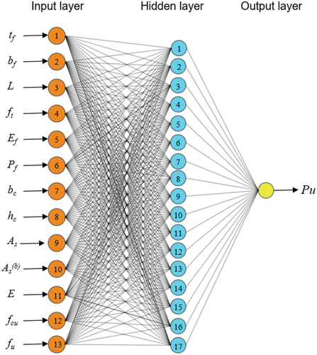
The modeling problem of predicting the flexural ultimate load capacity of prestressed FRP-RC is attributed to the nonlinear input-output relationship between the flexural ultimate load capacity of RC and its influencing factors. Thus, the problem of predicting the flexural ultimate load capacity of concrete is summarized as the establishment of a multi-input single-output network structure. Thirteen influencing factors, including the compressive strength of concrete, have been selected as the input layers of the neural network. The corresponding flexural ultimate load capacity of the RC beam after strengthening is used as the single output to build the network model. The key to determining the network structure is to select and determine the appropriate number of hidden layers and neurons. For given input and output layers, having too few hidden layers and neurons will readily lead to underfitting, that is, insufficient model fitting. Too many hidden layers and neurons will lead to overfitting, i.e., too strong model fitting (Guoliang 2021). Therefore, when determining the neural network structure, the number of hidden layers and neurons is an important factor that affects the prediction results. As this study is a simple data set that does not involve time series, the number of hidden layers is one, and the number of neurons in this hidden layer is based on the empirical formula:

(19) $\mathrm{h}=\sqrt{\mathrm{n}+\mathrm{m}}+\mathrm{c},\mathrm{c}\in \left[1,10\right]$(19)

where $\mathit{h}$ is the number of nodes in the hidden layer, $\mathit{n}$ is the number of nodes in the input layer, and $\mathit{m}$ is the number of nodes in the output layer.

Therefore, the number of neurons in the hidden layer is selected as between 4 and 22 based on the number of nodes in the input layer being 13 and the number of output nodes being 1. The BP neural network is taken as an example. The MSE, R, and average error percentage of the validation set are used as the evaluation indexes of the prediction results to find the optimal number of hidden layer nodes. The results are shown in Figure2(c). The best comprehensive performance is achieved with 17 neurons in the hidden layer, with an MSE of 0.023383, R of 0.94351, and the average error of 30.71%. This structure was used in L – M and BR neural networks to predict the flexural ultimate load capacity of RC beams. The validation set error at hidden layer node 17 is shown in Figure 2(d). Most of the validation set errors are concentrated around − 30%. The structure of the neural network model is illustrated in Figure 3. In this case, the input layer nodes are the 13 influencing factors of the ultimate flexural load of concrete, which is determined as 13, the number of hidden layers is 1 layer, the hidden layer nodes are 17, and the output layer has the ultimate flexural load of concrete as a single output node.

Figure 2. Performance of the BP neural network with different hidden layer nodes.

Figure 3. Prediction results of the prestressed FRP-RC flexural ultimate load neural network model.

4.2. Neural network parameters

The neural network parameters critically impact the performance and prediction results, so they need to be tuned for performance optimization. Four important parameters of the neural network are selected for tuning. The learning rate determines the step length and direction of the weight updates in each iteration. If the learning rate is too small, the network converges slowly and requires many iterations to achieve a good fit. If the learning rate is too large, the weights may oscillate and fail to converge to the global optimal solution. The momentum coefficient accelerates the convergence process and enhances the network stability. The network may fail to converge or overfit if the momentum coefficient is too large. If the momentum coefficient is too small, the convergence speed of the network may be reduced and it may easily get stuck at local optima. The regularization coefficient can control the network complexity and prevent overfitting. A regularization coefficient that is too large may lead to underfitting. A regularization factor that is too small may not be able to effectively control the network complexity, affecting the generalization ability. The number of iterations determines the rounds required for training. If there are too few iterations, the desired fitting effect may not be achieved. Too many iterations may lead to overfitting or excessive training times.

The validation set MSE is used as the performance evaluation index of the neural network to observe the effects of variations in the four parameters on the performance. One parameter is adjusted while the others are held constant as default values. The BR neural network is based on the principle of Bayesian statistics, effectively avoiding overfitting by introducing an a priori distribution to control the weight update compared with traditional neural networks. The BR neural network does not necessarily use the validation set for model selection and tuning and instead uses the default parameters. Therefore, this paper only tuned the four parameters in the BP and L – M neural networks. The results are shown in Figure 4.

Figure 4. Effect of parameter changes on the performance of the neural network models.

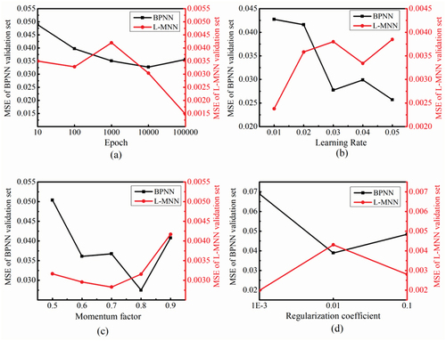
The optimal parameters for each network are shown in Table 1. This paper utilizes the sigmoid function as $\mathit{f}\left(\mathit{x}\right)=1/\left(1+\mathit{exp}\left(-\mathit{x}\right)\right)$ for the neural activation, which returns a value from 0 to 1 in the output layer. The BP neural network achieves the best MSE values for the validation set at 10,000 epochs, learning rate of 0.05, momentum factor of 0.8, and regularization factor of 0.01. The optimal MSE values for a single parameter control were 0.0327, 0.0257, 0.02748, and 0.0389, respectively. The L – M neural network achieved the optimal MSE values for the validation set with 100,000 epochs, learning rate of 0.01, momentum factor of 0.7, and regularization factor of 0.001. The optimal MSE values under a single parameter control were 0.001475, 0.00238, 0.002829, and 0.00198, respectively.

Table 1. Model architectures of the considered neural networks.

Parameter	BPNN	L-MNN	BRNN
Activation Function	sigmoid	sigmoid	sigmoid
Number of Input Layers	13	13	13
Number of Hidden Layers	1	1	1
Hidden Layer Size	17	17	17
Number of Output Layers	1	1	1
Epochs	10,000	100,000	/
Learning Rate	0.05	0.01	/
Momentum Factor	0.8	0.7	/
Regularization Coefficient	0.01	0.001	/

5. Neural network simulations

5.1. Prediction performance of neural network models

After determining the neural network structure and parameters, the flexural ultimate loads of the prestressed FRP-RC are predicted using the L – M and BR neural networks. The prediction results are compared with experimental values, as shown in Figures 5 and 6, and the error percentage distributions are shown in Figures 7 and 8.

Figure 5. Predicted values from the L–M neural network.

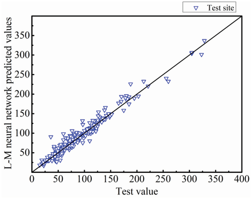
Figure 6. Predicted values from the BR neural network.

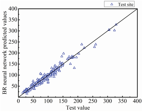
Figure 7. L-MNN prediction percentage error distribution.

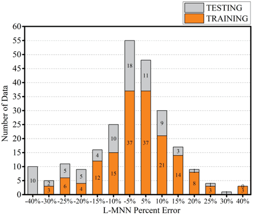
Figure 8. BRNN prediction percentage error distribution.

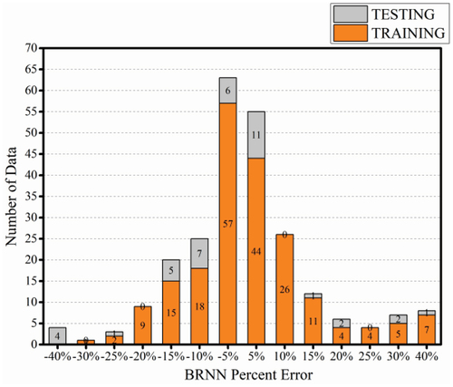
From Figures 5 and 6, the prediction results of both the L – M and BR neural networks are similar to the experimental values. From Figures 7 and 8, More than 65% of the prediction error percentages for L-M and BR neural networks are in the interval [−10%, 10%] and more than 85% of the prediction error percentages are in the interval [−20%, 20%]. Table 2 compares the prediction results of the conventional BP, L – M, and BR neural networks. While the average error of the conventional BP neural network is 30.15%, the average errors of the L-M and BR neural networks decrease to 10.468% and 8.794%, respectively, giving considerable improvements. The prediction results and performance metrics are illustrated using violin plots and Taylor plots in Figures 9 and 10, respectively, to better compare the prediction results of the three neural networks. In the Taylor plots, In the Taylor plot, the standard deviation of the test values = 0.1696315 with MSE = 0 and R = 1 used as plotting references. The BR neural network has a better prediction performance than the other two networks.

Figure 9. Violin plots of each neural network versus test values.

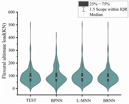
Figure 10. Taylor diagram for each neural network.

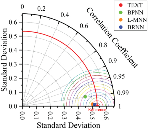
Table 2. Neural network performance comparisons.

Prediction method	MAPE	MAE	MSE	RMSE	R	Time
BPNN	30.15%	0.04343	0.02338	0.15029	0.94351	4.7
L-MNN	10.47%	0.01575	0.00161	0.04009	0.96619	1
BRNN	8.79%	0.01455	0.00051	0.02259	0.97972	9.4

5.2. Input variable contributions to the output variable

Analysis of contributions of the input variables was carried out to investigate the influence of the input variables on the output variable and thus to have a comprehensive understanding of the prediction models. The input variable contribution can be evaluated using the relative importance (RI), which can be calculated using the analysis method proposed by Garson (Garson 1991) as presented in Eq. (19)(19) $\mathrm{h}=\sqrt{\mathrm{n}+\mathrm{m}}+\mathrm{c},\mathrm{c}\in \left[1,10\right]$(19) . Based on the analysis of the prediction performance of the three neural networks, the contribution of the input variables to the output variables is analyzed with the best-performing BR neural network. The weights and biases of the BRNN model are extracted as follows:

$\begin{array}{rl}& w_1=\left(\begin{array}{ccccccccccccc}-0.3735& -0.0708& -0.2651& 0.4648& 0.2200& 0.2091& 0.0868& 0.0348& -0.1131& -0.1283& -0.7176& -0.2789& -0.3031\\ 0.0272& -0.0272& 0.0022& 0.0092& 0.0009& 0.0257& 0.0141& 0.001& 0.0407& 0.0073& 0.0305& 0.0212& 0.0168\\ -0.0022& -0.0038& -0.0092& -0.0009& -0.0257& -0.0141& -0.001& -0.0407& -0.0073& -0.0073& -0.0305& -0.0212& -0.0168\\ 0.0272& 0.0022& 0.0038& 0.0092& 0.0009& 0.0257& 0.0141& 0.001& 0.0407& 0.0073& 0.0305& 0.0212& 0.0168\\ -0.0272& -0.0022& -0.0038& -0.0092& -0.0009& -0.0257& -0.0141& -0.001& -0.0407& -0.0073& -0.0305& -0.0212& -0.0168\\ -0.2865& -0.2065& -0.6761& 0.2380& -0.4023& 0.1226& 0.4350& 0.8261& -0.1922& -0.4273& 0.7890& 0.1396& -0.0446\\ 0.0571& -0.1953& -0.1399& -0.0068& -0.1075& -0.0909& -0.4684& -0.6396& 0.1026& 0.7069& 0.3486& -0.9218& 0.5634\\ 0.3818& -0.0025& -0.1082& 0.3134& -0.0020& -0.0484& -0.3092& -0.1659& 0.2005& 0.3918& 0.2408& 0.1104& 0.4011\\ 0.0272& 0.0022& 0.0038& 0.0009& 0.0257& 0.0141& 0.0001& 0.0407& 0.0073& 0.0305& 0.0305& 0.0212& 0.0168\\ 0.1691& 0.1083& 0.2986& -0.0054& 0.1382& 0.2198& -0.3584& 0.0466& -0.7759& 0.2761& 0.1396& -0.1174& -0.3091\\ 0.0272& 0.0022& 0.0038& 0.0092& 0.0009& 0.0257& 0.0141& 0.0001& 0.0407& 0.0073& 0.0305& 0.0212& 0.0168\\ -0.2443& -0.1859& -0.0923& 0.1762& 0.4703& -0.2931& 0.5400& 0.5533& -0.3389& 0.7114& 0.5236& -0.8759& 0.0703\\ -0.4366& -0.2996& -0.3613& 0.3313& -0.0929& 0.4619& -0.5160& 0.4404& -0.2059& 0.4818& -0.2920& -0.3151& -0.7825\\ -0.2627& -0.2179& 0.3293& 0.2727& 0.4027& -0.3486& 0.7076& 0.1848& 0.4950& 0.2168& 0.0344& -0.0998& 0.0218\\ -0.0272& -0.0022& -0.0038& -0.0092& -0.0009& -0.0257& -0.0141& -0.0001& -0.0407& -0.0073& -0.0305& -0.0212& -0.0168\\ 0.0272& 0.0022& 0.0038& 0.0092& 0.0009& 0.0257& 0.0141& 0.0001& 0.0407& 0.0073& 0.305& 0.0212& 0.0168\\ 0.3034& -0.1796& -0.1151& 0.2748& 0.2720& -0.3170& -0.2345& 0.0767& -0.1942& 0.0376& -0.1583& 0.1236& -0.1698\end{array}\right)b_1=\left(\begin{array}{c}-0.1919\\ -0.0196\\ \mathit{\hspace{0.17em}}0.0196\\ -0.0196\\ \mathit{\hspace{0.17em}}0.0196\\ -0.5790\\ 0.2279\\ 0.0426\\ -0.0196\\ -0.1866\\ -0.0196\\ -0.1135\\ 0.4073\\ 0.1671\\ 0.0196\\ -0.0196\\ 0.1041\end{array}\right)\\ & w_2=\left(-0.86870.0752-0.07520.0752-0.0752-1.0285-1.2790.80850.0752-0.79880.07521.01211.0447-0.8291-0.07520.0752-0.6167\right)\\ & b_2=-0.2814\end{array}$

where w₁ is the weight matrix of the input layer to the hidden layer, b₁ is the bias vector of the hidden layer, w₂ is the weight vector of the hidden layer to the output layer and b₂ is the bias of the output layer.

(20) $\mathit{R}{I}_i=\frac{\sum _{\mathit{j}=1}^K[(\left|w_{1,\mathit{ij}}\right|/\sum _{\mathit{r}=1}^N\left|w_{1,\mathit{rj}}\right|)\left|w_{2,\mathit{j}}\right|]}{\sum _{\mathit{i}=1}^N\left\{\sum _{\mathit{j}=1}^K[(\left|w_{1,\mathit{ij}}\right|/\sum _{\mathit{r}=1}^N\left|w_{1,\mathit{rj}}\right|)\left|w_{2,\mathit{j}}\right|]\right\}}$(20)

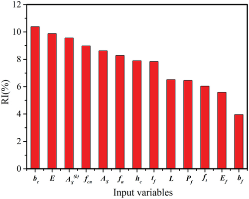
where $\mathit{R}{I}_i$ represents the RI to the $\mathit{i}$th input variable, $w_{1,\mathit{ij}}$ is the connection between the $\mathit{i}$th input variable and $\mathit{j}$th neuron in the hidden layer, $w_{2,\mathit{j}}$ is the connection between the $\mathit{j}$th neuron in the hidden layer and the output variable, and $\mathit{N}$ and $\mathit{K}$ are the numbers of input variables and neurons in the hidden layer, respectively. Figure 11 illustrates the RI of the input variables in the BRNN model. Among the 13 influencing factors, the ones that are more impactful are from the concrete. The beam width, concrete modulus of elasticity, and the lower reinforcement have the greatest influences on the flexural load-carrying capacity with RIs of 10.38%, 9.88%, and 9.56%, respectively. In contrast, the characteristic importance of the FRP sheet width, modulus of elasticity, and tensile strength are lower at 3.96%, 5.59%, and 6.04%, respectively. None of the FRP reinforcement parameters are determining factors for the flexural load-carrying capacity of RC beams. The phenomenon is reasonable as the effect of the FRP reinforcement is only mentioned based on the original flexural load capacity of the RC beams, while the decisive role is still played by the initial beam parameters (Liu et al. 2017; Zhao et al. 2018). Among the relevant parameters of the FRP, the width and length are the most influential on the reinforcement effect, which coincides with the results of the relevant FRP-RC beam tests (Yang 2006).

Figure 11. Relative importance of the input variables for the BRNN model.

5.3. Decomposition method to handle noisy data

The SVD techniques are utilized to eliminate noisy data from the input layer data and observe changes in the neural network performance (Razzaghi, Madandoust, and Aghabarati 2021). The SVD is widely used in the field of ML. It is not only used for feature decomposition in dimensionality reduction but also for recommendation systems, natural language processing, and others. This is the cornerstone of many ML algorithms. The SVD decomposes the training data matrix to obtain three matrices $\mathit{U}$, $\mathit{D}$, and $\mathit{V}$ that combine to achieve the original matrix as:

(21) $\mathit{A}=\mathit{UD}{V}^T$(21)

A threshold of 0.01 is chosen in which all terms in $\mathit{D}$ with singular values less than the threshold are set to 0 to construct the diagonal matrix $D^{\prime }$. The original matrix $\mathit{A}$ is updated using $D^{\prime }$ to obtain the matrix:

(22) $\mathit{A}{ }^{\mathrm{\prime }}=\mathit{UD}{ }^{\mathrm{\prime }}{V}^T$(22)

This new matrix $\mathit{A}{ }^{\mathrm{\prime }}$ is called the denoised matrix and provides the data to retrain the neural network model. Based on the above method, the 13 × 243 input layer matrix containing 13 input layer variables is set up as A. It is SVD decomposed into A^’ matrix and then reintroduced into each neural network model to predict the flexural ultimate load of concrete. The R and MSE are used as the performance evaluation indexes of the neural network, as shown in Table 3, indicating the performance of each neural network has improved. The BP neural network has the largest performance improvement with a 17.59% reduction in MSE and a 1.724% increase in R.

Table 3. Performance change before and after SVD optimization.

Prediction method	MSE	MSE after SVD optimization	R	R after SVD optimization
BPNN	0.02338	0.01927	0.94351	0.95978
L-MNN	0.00161	0.00136	0.96619	0.97073
BRNN	0.00051	0.00046	0.97972	0.98171

6. Conclusion

Select ANN models based on three algorithms are used to predict the ultimate flexural loads of prestressed FRP sheets for RC beams. The performances of the three neural networks were evaluated after determining the effects of the network structure and parameters. BR neural network prediction was identified as a method that can accurately predict the flexural ultimate bearing capacity loads of prestressed FRP-RC. The contributions of the input variables were analyzed, and the SVD method was used to eliminate noisy data in the input layer. The following conclusions are drawn based on the results.

• The optimal hidden layer nodes for the three neural networks were determined to be 17 using the MSE value, R-value, and average error of the validation set as evaluation metrics. The optimal parameters of BP neural network and L-M neural network were determined using the MSE value of the validation set as an evaluation metric. The BP neural network achieves the best MSE values for the validation set at 10,000 epochs, learning rate of 0.05, momentum factor of 0.8, and regularization factor of 0.01. The L-M neural network achieved the optimal MSE values for the validation set with 100,000 epochs, learning rate of 0.01, momentum factor of 0.7, and regularization factor of 0.001. The BR neural network will update the parameter distributions during training through Bayesian inference, so no parameter tuning is performed.

• Based on the determined neural network structure and parameters, the ultimate flexural load of prestressed FRP-RC is predicted using BP neural network, L-M neural network, and BR neural network. The performance of the BR neural network (accuracy rate = 91.21% and MSE = 0.00051) is better than BP neural network (accuracy rate = 69.85% and MSE = 0.02338) and L-M neural network (accuracy rate = 89.53% and MSE = 0.00161). The BR neural network was determined to be the best neural network.

• After determining the accuracy of the prediction models, a feature importance analysis was performed using the weights and thresholds of the BR neural network to justify the model. The beam width, concrete modulus of elasticity, and bottom reinforcement were the most influential factors on the flexural capacity of the RC beam, with RI of 10.38%, 9.88%, and 9.56%, respectively. Among the parameters related to the FRP reinforcement, the width and length of the FRP and applied prestress had the greatest influences on the reinforcement effectiveness, with RI of 7.84%, 6.52%, and 6.45%, respectively. Experimenters may consider prioritizing parameters that have high impacts on the flexural ultimate load to improve the flexural performance of concrete beams.

• The three neural network models were then trained after eliminating noisy data in the input layer using the SVD method. The results showed that the performances of all three neural network models improved to some extent, with the BP neural network showing the largest improvement with a 17.59% decrease in the MSE and a 1.724% increase in R.

Although the model exhibits good performance, there are still some shortcomings. The prediction accuracy should be improved by collecting additional data or considering increasing the number of influencing factors in the input layer. All proposed models use the most common sigmoid function in all layers. The proposed models can be evaluated using other activation functions (such as linear, tangent hyperbolic, and ReLU). The neural network model for the conventional algorithm is still used, and an advanced hybrid dynamic model or other advanced models can be considered to predict the flexural ultimate load of concrete beams, which may lead to higher accuracies.

Disclosure statement

No potential conflict of interest was reported by the author(s).

Additional information

Funding

This work was supported by the The National Natural Science Foundation of China [No.52208244]; The Scientific and Technological Research Projects in Henan Province [No.222102320034].

APPENDIX

Table

	FRP sheet						Reinforced concrete beam
Sample ID	Width	Thickness	Bond length	Tensile strength	Modulus of elasticity	Prestressed	Width	Height	Area of reinforcement		Modulus of elasticity	Concrete compressive strength	Concrete tensile strength	Ultimate load
	tf	bf	L	ff	Ef	Pf	bc	hc	top	bottom	E	fck	ftk
	(mm)	(mm)	(mm)	(MPa)	(MPa)	(MPa)	(mm)	(mm)	As/mm^2	As^(b)/mm^2	(MPa)	(MPa)	(MPa)	Pu (kN)
1	0	0	0	0	0	0	150	250	101	226	25500	13.4	1.54	37
2	0	0	0	0	0	0	150	250	101	461	30000	20.1	2.01	102
3	0	0	0	0	0	0	150	250	101	760	32500	26.8	2.39	203
4	100	0.7	950	542	22000	0	150	250	101	226	25500	13.4	1.54	57
5	100	0.7	950	542	22000	0	150	250	101	226	25500	13.4	1.54	50
6	100	1.4	750	542	22000	0	150	250	101	461	25500	13.4	1.54	120
7	100	2.1	550	542	22000	0	150	250	101	760	25500	13.4	1.54	188
8	100	2.1	550	542	22000	0	150	250	101	760	25500	13.4	1.54	58
9	100	0.7	850	542	22000	0	150	250	101	226	30000	20.1	2.01	110
10	100	1.4	650	542	22000	0	150	250	101	461	30000	20.1	2.01	140
11	100	2.1	450	542	22000	0	150	250	101	760	30000	20.1	2.01	256
12	100	2.1	650	542	22000	0	150	250	101	461	30000	20.1	2.01	123
13	100	0.7	750	542	22000	0	150	250	101	226	32500	26.8	2.39	60
14	100	1.4	550	542	22000	0	150	250	101	461	32500	26.8	2.39	133
15	100	2.1	350	542	22000	0	150	250	101	760	32500	26.8	2.39	213
16	100	2.1	350	542	22000	0	150	250	101	760	32500	26.8	2.39	260
17	100	0.7	0	542	22000	0	150	250	101	226	25500	13.4	1.54	45
18	100	0.7	100	542	22000	0	150	250	101	226	30000	20.1	2.01	46
19	100	0.7	200	542	22000	0	150	250	101	226	32500	26.8	2.39	46
20	0	0	0	4000	230000	0	180	250	101	339	32000	29.8	2.51	60.4
21	120	2	2000	4000	230000	800	180	250	101	339	34000	32	2.64	68.2
22	120	4	1780	4000	230000	800	180	250	101	339	34000	32	2.64	89.2
23	160	4	1780	4000	230000	800	180	250	101	339	34000	31	2.64	92.3
24	160	4	1780	4000	230000	1000	180	250	101	339	34000	32	2.64	87.5
25	120	6	2360	4000	230000	800	200	300	101	339	36000	36.3	2.74	115.3
26	160	6	2360	4000	230000	1000	200	300	101	339	36000	37.6	2.74	119.6
27	150	0.167	2700	2100	270000	0	150	250	308	308	31200	32.79	2.58	42.5
28	150	0.167	2700	2100	270000	486	150	250	308	308	31200	32.79	2.58	76.2
29	150	0.167	2700	2100	270000	864	150	250	308	308	31200	32.79	2.58	70.6
30	150	0.167	2700	2100	270000	1242	150	250	308	308	31200	32.79	2.58	67.3
31	0	0	0	0	0	0	80	120	57	101	36000	69.84	2.85	44.8
32	110	0.334	480	3771	218000	0	80	120	57	101	36000	69.84	2.85	58.9
33	110	0.334	480	3771	218000	565.65	80	120	57	101	36000	69.84	2.85	63.6
34	110	0.334	480	3771	218000	1131.3	80	120	57	101	36000	69.84	2.85	72.3
35	0	0	0	0	0	0	120	180	157	226	36000	69.84	2.85	79.5
36	170	0.334	935	3771	218000	0	120	180	157	226	36000	69.84	2.85	100.1
37	170	0.334	935	3771	218000	565.65	120	180	157	226	36000	69.84	2.85	108.9
38	170	0.334	935	3771	218000	1131.3	120	180	157	226	36000	69.84	2.85	121.9
39	0	0	0	0	0	0	150	250	308	308	34600	50.07	3.11	18.88
40	150	0.167	2600	4330	227000	0	150	250	308	308	35100	53.45	3.11	26.47
41	150	0.167	2600	4330	227000	0	150	250	308	308	35100	53.45	3.11	32.82
42	150	0.167	2600	4330	227000	723.7	150	250	308	308	34600	50.07	3.11	30.72
43	150	0.167	2600	4330	227000	817.7	150	250	308	308	34600	50.07	3.11	29.51
44	150	0.167	2600	4330	227000	806.4	150	250	308	308	35000	52.69	3.11	35.16
45	150	0.167	2600	4330	227000	72.6	150	250	308	308	35000	52.69	3.11	30.12
46	150	0.167	2600	4330	227000	1070.9	150	250	308	308	35100	53.45	3.11	39.37
47	0	0	0	0	0	0	150	200	101	308	28500	26.50	2.39	62.5
48	150	4	200	191.56	11580	22.04	150	200	101	308	28500	26.50	2.39	99.6
49	0	0	0	0	0	0	150	200	101	308	24340	18.18	2.01	57.2
50	150	4	200	191.56	11580	0	150	200	101	308	24340	18.18	2.01	80.9
51	150	4	200	191.56	11580	13.81	150	200	101	308	24340	18.18	2.01	86.8
52	150	4	200	191.56	11580	22.096	150	200	101	308	24340	18.18	2.01	87.5
53	150	4	200	191.56	11580	27.62	150	200	101	308	24340	18.18	2.01	77.8
54	0	0	0	0	0	0	150	300	157	226	31000	28.5	1.76	52.22
55	150	0.17	2800	3610	244000	0	150	300	157	226	30000	12.2	1.15	72.5
56	150	0.21	2800	2650	76000	0	150	300	157	226	30000	12.2	1.15	64.2
57	150	0.2	2800	3350	156000	0	150	300	157	226	30000	12.2	1.15	68.3
58	150	0.34	2800	3610	244000	0	150	300	157	226	30000	12.2	1.15	92.5
59	150	0.42	2800	2650	76000	0	150	300	157	226	30000	12.2	1.15	98.54
60	150	0.38	2800	3130	160000	0	150	300	157	226	30000	12.2	1.15	96.8
61	0	0	0	0	0	0	200	250	157	308	32500	26.8	2.39	71.23
62	200	2	2600	2155	81000	0	200	250	157	308	32500	26.8	2.39	80.15
63	200	6	2600	1906	88000	0	200	250	157	308	32500	26.8	2.39	98.11
64	200	2	2600	2155	81000	646.5	200	250	157	308	32500	26.8	2.39	84.51
65	200	2	2600	2155	81000	1077.5	200	250	157	308	32500	26.8	2.39	87.91
66	200	6	2600	1906	88000	571.8	200	250	157	308	32500	26.8	2.39	108.31
67	200	6	2600	1906	88000	953	200	250	157	308	32500	26.8	2.39	112.26
68	0	0	0	0	0	0	160	300	157	509	30000	31.89	2.64	98
69	50	1.2	3000	2360	151000	0	160	300	157	509	30000	31.89	2.64	125
70	50	1.2	3000	2360	151000	590	160	300	157	509	30000	33.7	2.64	135
71	50	1.2	3000	2360	151000	991.2	160	300	157	509	30000	33.7	2.64	129
72	50	1.2	3000	2360	151000	991.2	160	300	157	760	30000	35.62	2.64	185
73	50	1.2	3000	2360	151000	590	160	300	157	226	30000	35.62	2.64	90
74	0	0	0	0	0	0	120	250	101	226	28000	29.76	2.51	44
75	0	0	0	0	0	0	120	250	101	226	28000	24.75	2.20	40
76	90	0.111	2200	3055	235000	0	120	250	101	226	28000	23.63	2.20	49
77	90	0.111	2200	3055	235000	0	120	250	101	226	28000	30.00	2.51	52
78	120	0.111	2200	3055	235000	0	120	250	101	226	28000	28.07	2.51	58
79	120	0.111	2200	3055	235000	0	120	250	101	226	28000	30.10	2.51	60
80	90	0.111	2200	3055	235000	2490	120	250	101	226	28000	28.02	2.51	55
81	90	0.111	2200	3055	235000	4800	120	250	101	226	28000	26.37	2.39	60
82	90	0.111	2200	3055	235000	5230	120	250	101	226	28000	24.98	2.20	55
83	120	0.111	2200	3055	235000	2150	120	250	101	226	28000	26.82	2.39	69
84	120	0.111	2200	3055	235000	5000	120	250	101	226	28000	30.51	2.51	69
85	120	0.111	2200	3055	235000	2985	120	250	101	226	28000	26.82	2.39	65
86	120	0.111	2200	3055	235000	5194	120	250	101	226	28000	29.20	2.51	71
87	0	0	0	0	0	0	120	240	101	339	30000	20	2.01	36
88	100	0.167	2000	3400	240000	0	120	240	101	339	30000	19	2.01	82
89	100	0.167	2000	3400	240000	59.9	120	240	101	339	30000	18	2.01	84
90	100	0.167	2000	3400	240000	89.8	120	240	101	339	30000	19	2.01	92
91	0	0	0	0	0	0	120	240	101	452	30000	23	2.01	47
92	100	0.167	2000	3400	240000	0	120	240	101	452	30000	21	2.01	88
93	100	0.167	2000	3400	240000	59.9	120	240	101	452	30000	23	2.01	102
94	100	0.167	2000	3400	240000	89.8	120	240	101	452	30000	22	2.01	112
95	0	0	0	0	0	0	120	250	157	628	33535.2	42.25	3.15	150
96	50	1.2	1200	2461	165000	0	120	250	157	628	33535.2	42.25	3.15	165
97	50	1.2	1200	2461	165000	246.1	120	250	157	628	33535.2	42.25	3.15	170
98	50	1.2	1200	2461	165000	492.2	120	250	157	628	33535.2	42.25	3.15	180
99	50	1.2	1200	2461	165000	738.3	120	250	157	628	33535.2	42.25	3.15	195
100	50	1.2	1200	2461	165000	984.4	120	250	157	628	33535.2	42.25	3.15	185
101	50	1.2	1200	2461	165000	1230.5	120	250	157	628	33535.2	42.25	3.15	180
102	0	0	0	0	0	0	300	500	0	1571	40300	50.2	2.64	110
103	250	0.167	4600	4500	230000	0	300	500	0	1571	40300	50.2	2.64	110
104	250	0.167	4600	4500	230000	1078	300	500	0	1571	40300	50.2	2.64	175
105	250	0.167	4600	4500	230000	1317	300	500	0	1571	40300	50.2	2.64	140
106	60	0.111	3055	2500	235000	75.19	120	250	101	226	28000	26.6	1.78	49.1
107	60	0.111	3055	2500	235000	303.5	120	250	101	226	28000	26.6	1.78	50.7
108	60	0.111	3055	2500	235000	658.24	120	250	101	226	28000	26.6	1.78	49.6
109	70	0.167	2904	2500	220000	68.91	120	250	101	226	28000	26.6	1.78	54.2
110	70	0.167	2904	2500	220000	266.64	120	250	101	226	28000	26.6	1.78	56.2
111	70	0.167	2904	2500	220000	620	120	250	101	226	28000	26.6	1.78	56.9
112	120	0.167	2904	2500	220000	69.85	120	250	101	226	28000	26.6	1.78	60.9
113	120	0.167	2904	2500	220000	286.68	120	250	101	226	28000	26.6	1.78	63.9
114	120	0.167	2904	2500	220000	617.65	120	250	101	226	28000	26.6	1.78	67.0
115	0	0	0	0	0	0	350	500	339	951	30000	26.8	2.01	221.3
116	200	0.334	4000	2625	164000	0	350	500	339	951	30000	26.8	2.01	305
117	100	1.4	4000	2625	164000	720	350	500	339	951	30000	26.8	2.01	323.1
118	100	1.4	4000	2625	164000	960	350	500	339	951	30000	26.8	2.01	304.6
119	100	1.4	4000	2625	164000	1200	350	500	339	951	30000	26.8	2.01	304.8
120	0	0	0	0	0	0	150	200	101	308	28500	26.5	2.39	62.5
121	100	4	2000	191.56	11580	22.04	150	200	101	308	28500	26.5	2.39	99.6
122	0	0	0	0	0	0	150	200	101	308	24300	18.2	2.01	57.24
123	100	4	2000	191.56	11580	0	150	200	101	308	24300	18.2	2.01	80.88
124	100	4	2000	191.56	11580	13.81	150	200	101	308	24300	18.2	2.01	86.8
125	100	4	2000	191.56	11580	22.09	150	200	101	308	24300	18.2	2.01	87.5
126	100	4	2000	191.56	11580	27.616	150	200	101	308	24300	18.2	2.01	77.8
127	0	0	0	0	0	0	120	200	101	308	30000	40.4	2.85	56.94
128	100	0.386	2100	2000	90000	0	120	200	101	308	30000	40.4	2.85	85.26
129	100	0.386	2100	2000	90000	925	120	200	101	308	30000	40.4	2.85	92.37
130	100	0.193	2100	2060	118000	0	120	200	101	308	30000	40.4	2.85	63.24
131	100	0.386	2100	2060	118000	778	120	200	101	308	30000	40.4	2.85	68.50
132	0	0	0	0	0	0	150	300	57	226	28000	19.45	2.26	26
133	150	0.167	2800	3700	246000	0	150	300	57	226	28000	19.45	2.26	60
134	150	0.167	2800	3700	246000	600	150	300	57	226	28000	19.45	2.26	80
135	0	0	0	0	0	0	150	300	57	226	28000	18.54	2.19	54
136	150	0.167	2800	3700	246000	0	150	300	57	226	28000	18.54	2.19	100
137	150	0.167	2800	3700	246000	600	150	300	57	226	28000	18.54	2.19	100
138	0	0	0	0	0	0	150	250	57	157	25500	24.5	2.20	22.5
139	100	0.167	3000	3550	235000	0	150	250	57	157	25500	24.5	2.20	26.25
140	100	0.167	3000	3550	235000	0	150	250	57	157	25500	24.5	2.20	26.5
141	100	0.167	3000	3500	235000	479.04	150	250	57	157	25500	24.5	2.20	30.25
142	100	0.167	3000	3550	235000	718.56	150	250	57	157	25500	24.5	2.20	27.5
143	100	0.167	3000	3550	235000	958.08	150	250	57	157	25500	24.5	2.20	31.25
144	100	0.167	3000	3550	235000	1077.84	150	250	57	157	25500	24.5	2.20	38.3
145	100	0.167	3000	3550	235000	598.80	150	250	57	157	25500	24.5	2.20	33
146	100	0.167	1940	2941	207000	0	100	150	101	57	32000	25	2.35	19
147	100	0.167	1940	2941	207000	0	100	150	101	57	32000	25	2.35	22.5
148	100	0.167	1940	2941	207000	1046	100	150	101	57	32000	25	2.35	28
149	100	0.167	1940	2941	207000	1046	100	150	101	57	32000	25	2.35	26
150	100	0.167	1940	2941	207000	588	100	150	101	57	32000	25	2.35	21.5
151	100	0.167	1940	2941	207000	1438	100	150	101	57	32000	25	2.35	25
152	0	0	0	0	0	0	200	300	339	236	28000	16.4	1.78	49.4
153	50	1.3	2400	2350	173000	0	200	300	339	236	28000	16.4	1.78	121.5
154	50	1.3	2400	2350	173000	470	200	300	339	236	28000	16.4	1.78	123.0
155	50	1.3	2400	2350	173000	940	200	300	339	236	28000	16.4	1.78	125.2
156	50	1.3	2400	2350	173000	1410	200	300	339	236	28000	16.4	1.78	122.8
157	50	1.3	4500	2350	173000	1410	200	300	339	236	28000	16.4	1.78	121.4
158	50	1.3	6000	2350	173000	1410	200	300	339	236	28000	16.4	1.78	71.8
159	0	0	0	0	0	0	150	300	308	308	30000	19.8	2.01	87
160	150	0.111	2400	4286	256000	0	150	300	308	308	34500	33.0	2.64	118
161	150	0.111	2400	4286	256000	534.53	150	300	308	308	30000	19.8	2.01	137
162	150	0.111	2400	4286	256000	708.86	150	300	308	308	28000	15.9	1.78	111
163	150	0.111	2400	4286	256000	847.87	150	300	308	308	30000	19.8	2.01	119
164	150	0.111	2400	4286	256000	1120	150	300	308	308	30000	19.8	2.01	133
165	80	0.111	2400	4286	256000	1146.62	150	300	308	308	30000	21.9	2.01	103
166	120	0.111	2400	4286	256000	1063.94	150	300	308	308	34500	33.0	2.64	110
167	150	0.111	2400	4286	256000	704	150	300	308	308	34500	33.0	2.64	116
168	150	0.111	2400	4286	256000	7117.82	150	300	308	308	34500	33.0	2.64	121
169	150	0.111	2400	4286	256000	1092.1	150	300	308	308	34500	33.0	2.64	115
170	150	0.111	2400	4286	256000	1102.59	150	300	308	308	31500	24.0	2.20	116
171	0	0	0	0	0	0	150	350	760	402	30000	37.6	2.80	82
172	32	2	2900	2068	131000	0	150	350	760	402	30000	32.1	2.64	126.2
173	50	1.2	2900	3100	165000	1000	150	350	760	402	30000	26.6	2.39	146.4
174	32	2	2900	3100	165000	1000	150	350	760	402	30000	30.4	2.51	141.7
175	16	4.5	2900	3100	165000	1000	150	350	760	402	30000	35.5	2.74	97
176	32	2	3300	3100	165000	1000	150	350	760	402	30000	60.8	3.31	182
177	32	2	2900	3100	165000	1000	150	350	760	402	30000	59.5	3.29	178
178	0	0	0	0	0	0	150	300	308	308	35600	52.8	3.11	47.3
179	140	0.167	1800	3522	259000	0	150	300	308	308	35600	52.8	3.11	77.9
180	140	0.167	1800	3522	259000	1267.92	150	300	308	308	35600	52.8	3.11	80.7
181	140	0.167	1800	3522	259000	1408.8	150	300	308	308	35600	52.8	3.11	81.9
182	140	0.167	1800	3522	259000	1761	150	300	308	308	35600	52.8	3.11	84.6
183	140	0.167	1800	3522	259000	2113.2	150	300	308	308	35600	52.8	3.11	85.3
184	140	0.334	1800	3522	259000	2113.2	150	300	308	308	35600	52.8	3.11	115.0
185	140	0.334	1800	3522	259000	2113.2	150	300	308	308	35600	52.8	3.11	116.0
186	0	0	0	0	0	0	100	100	57	85	35000	54	2.5	14.85
187	65	0.8	1000	1414	111000	0	100	100	57	85	35000	54	2.5	34
188	65	0.8	1000	1414	111000	0	100	100	57	85	35000	54	2.5	49.65
189	65	0.8	1000	1414	111000	332.29	100	100	57	85	35000	54	2.5	49.6
190	65	0.8	1000	1414	111000	335.12	100	100	57	85	35000	54	2.5	43.65
191	65	0.8	1000	1414	111000	667.41	100	100	57	85	35000	54	2.5	50.5
192	0	0	0	0	0	0	145	230	101	226	35000	47	2.6	28.5
193	0	0	0	0	0	0	145	230	101	339	35000	47	2.6	42.3
194	90	1.3	4500	1248	115000	0	145	230	101	226	35000	47	2.6	60
195	90	1.3	4500	1248	115000	330.72	145	230	101	226	35000	47	2.6	63.8
196	90	1.3	4500	1248	115000	326.98	145	230	101	339	35000	47	2.6	70.5
197	90	1.3	4500	1248	115000	419.33	145	230	101	339	35000	47	2.6	72.8
198	90	1.3	4500	1248	115000	581.57	145	230	101	339	35000	47	2.6	76.5
199	0	0	0	0	0	0	200	400	157	532	36000	46	2.99	84
200	32	2	5000	2610	145000	0	200	400	157	532	36000	46	2.99	135
201	32	2	5000	2610	145000	522	200	400	157	532	36000	43	2.99	148
202	32	2	5000	2610	145000	1044	200	400	157	532	36000	40	2.99	149
203	32	2	5000	2610	145000	1566	200	400	157	532	36000	40	2.99	149
204	0	0	0	0	0	0	200	300	236	400	30000	18.55	2.65	50.5
205	50	1.4	2400	2161	165000	0	200	300	236	400	30000	18.55	2.65	76.4
206	100	1.4	2400	2161	165000	0	200	300	236	400	30000	18.55	2.65	96.4
207	50	1.4	2400	2161	165000	0	200	300	236	400	30000	18.55	2.65	121.5
208	50	1.4	2400	2161	165000	432.2	200	300	236	400	30000	18.55	2.65	123.0
209	50	1.4	2400	2161	165000	864.4	200	300	236	400	30000	18.55	2.65	125.2
210	50	1.4	2400	2161	165000	1296.6	200	300	236	400	30000	18.55	2.65	122.8
211	50	1.4	2400	2161	165000	1512.7	200	300	236	400	30000	18.55	2.65	126.5
212	0	0	0	0	0	0	400	600	853	1900	30000	18.55	2.65	328.5
213	100	1.4	6000	2161	165000	1080.5	400	600	853	1900	30000	18.55	2.65	502.1
214	0	0	0	0	0	0	220	400	157	603	32500	26.4	2.39	74.1
215	50	1.4	2400	2850	165000	0	220	400	157	603	32500	26.4	2.39	89.6
216	50	1.4	2400	2850	165000	1140	220	400	157	603	32500	26.4	2.39	112.7
217	50	1.4	2400	2850	165000	1710	220	400	157	603	32500	26.4	2.39	118.4
218	50	1.4	2400	2850	165000	2280	220	400	157	603	32500	26.4	2.39	125.1
219	50	1.4	2400	2850	165000	1140	220	400	157	236	32500	26.4	2.39	81.7
220	50	1.4	2400	2850	165000	1710	220	400	157	236	32500	26.4	2.39	87.3
221	50	1.4	2400	2850	165000	2280	220	400	157	236	32500	26.4	2.39	90.6
222	50	1.4	2400	2850	165000	1710	220	400	157	400	32500	26.4	2.39	109.2
223	50	1.4	2400	2850	165000	2280	220	400	157	400	32500	26.4	2.39	116.3
224	50	1.4	2400	2850	165000	1710	220	400	157	1137	32500	26.4	2.39	146.0
225	50	1.4	2400	2850	165000	2280	220	400	157	1137	32500	26.4	2.39	151.9
226	50	1.4	2400	2850	165000	1710	220	400	157	603	30000	20.6	2.01	111.7
227	50	1.4	2400	2850	165000	2280	220	400	157	603	30000	20.6	2.01	121.9
228	50	1.4	2400	2850	165000	1710	220	400	157	603	35500	35.6	2.74	126.2
229	50	1.4	2400	2850	165000	2280	220	400	157	603	35500	35.6	2.74	126.8
230	50	1.4	2400	2850	165000	1995	220	400	157	236	37000	44.1	2.99	105.3
231	50	1.4	2400	2850	165000	1995	220	400	157	400	37000	44.1	2.99	125.4
232	50	1.4	2400	2850	165000	1995	220	400	157	603	37000	44.1	2.99	138.3
233	50	1.4	2400	2850	165000	1995	220	400	157	1137	37000	44.1	2.99	170.5
234	50	1.4	2500	2500	150000	1052	150	250	57	421	32500	52.3	3.6	63
235	20	1.4	2500	2500	150000	1102	150	250	57	421	32500	52.3	3.6	49
236	20	1.4	2500	2500	150000	1265	150	250	57	339	32500	52.3	3.6	44
237	20	1.4	2500	2500	150000	787	150	250	57	509	32500	52.3	3.6	53
238	20	1.4	2500	2500	150000	1087	150	250	57	509	32500	52.3	3.6	55
239	0	0	0	0	0	0	90	180	226	226	34500	32	2.64	102
240	50.8	1.4	1500	2510	155000	125.5	90	180	226	226	34500	32	2.64	100
241	50.8	1.4	1500	2510	155000	251	90	180	226	226	34500	32	2.64	105
242	50.8	1.4	1500	2510	155000	376.5	90	180	226	226	34500	32	2.64	108
243	50.8	1.4	1500	2510	155000	502	90	180	226	226	34500	32	2.64	115

References

- Adnan, R. M., O. Kisi, R. R. Mostafa, A. N. Ahmed, and A. El-Shafie. 2022. “The Potential of a Novel Support Vector Machine Trained with Modified Mayfly Optimization Algorithm for Streamflow Prediction.” Hydrological Sciences Journal 67 (2): 161–174. https://doi.org/10.1080/02626667.2021.2012182.
- Adnan, R. M., R. R. Mostafa, A. Elbeltagi, Z. M. Yaseen, S. Shahid, and O. Kisi. 2022. “Development of New Machine Learning Model for Streamflow Prediction: Case Studies in Pakistan.” Stochastic Environmental Research and Risk Assessment: Research Journal 36 (4): 999–1033. https://doi.org/10.1007/s00477-021-02111-z.
- Adnan, R. M., R. R. Mostafa, A. R. M. T. Islam, O. Kisi, A. Kuriqi, and S. Heddam. 2021. “Estimating Reference Evapotranspiration Using Hybrid Adaptive Fuzzy Inferencing Coupled with Heuristic Algorithms.” Computers and Electronics in Agriculture 191:106541. https://doi.org/10.1016/j.compag.2021.106541.
- Ahmad, A. 2020 8. Framework for the Development of Artificial Neural Networks for Predicting the Load Carrying Capacity of RC Members. University of Engineering and Technology.
- Akinosho, T. D., L. O. Oyedele. 2020. Deep Learning in the Construction Industry: A Review of Present Status and Future Innovations. Journal of Building Engineering 32:101827.
- Bhagwat, Y., G. Nayak, R. Bhat, and M. Kamath. 2023. “A Prediction Model for Flexural Strength of Corroded Prestressed Concrete Beam Using Artificial Neural Network.” Cogent Engineering 10:1 (1): 2187657. https://doi.org/10.1080/23311916.2023.2187657.
- Botchkarev, A. 2019. “A New Typology Design of Performance Metrics to Measure Errors in Machine Learning Regression Algorithms.” Interdisciplinary Journal of Information, Knowledge, and Management 14:045–076. https://doi.org/10.28945/4184.
- Cascardi, A., F. Micelli, and M. Aiello. 2017. “An Artificial Neural Networks Model for the Prediction of the Compressive Strength of FRP-Confined Concrete Circular Columns.” Engineering Structures 140:199–208. https://doi.org/10.1016/j.engstruct.2017.02.047.
- Chen, H. 2009. “Testing of Flexural Performance of Prestressed CFRP Plate Reinforced Concrete Beams.” Journal of Guilin Institute of Technology 29 (1): 81–83.
- Congro, M., V. M. D. A. Monteiro, A. L. T. Brandão, B. F. D. Santos, D. Roehl, and F. D. A. Silva. 2021. “Prediction of the Residual Flexural Strength of Fiber Reinforced Concrete Using Artificial Neural Networks.” Construction and Building Materials 303:124502. https://doi.org/10.1016/j.conbuildmat.2021.124502.
- Dogan, A., and D. Birant. 2021. “Machine Learning and Data Mining in Manufacturing.” Expert Systems with Applications 166:114060. https://doi.org/10.1016/j.eswa.2020.114060.
- Du, W. W. 2005. Concrete Strength Prediction Model Based on Artificial Neural Network [D]. Hubei, Wuhan, China: School of Civil Engineering, Wuhan University of Technology.
- Fei, W., and S. Y. Jiang. 2003. “Experimental Study on Prestressed Carbon Fiber Cloth Reinforced Concrete Flexural Members.” Sichuan Construction Science Research 2003 (2): 42–45.
- Gaafar, M. A., and R. El-Hacha. 2008. Strengthening Reinforced Concrete Beams with Prestressed Near Surface Mounted FRP Strips [C]. Fourth International Conference on FRP Composites in Civil Engineering, Zurich, Switzerland.
- Gao, P., X. Gu, and A. S. Mosallam. 2016. “Flexural Behavior of Preloaded Reinforced Concrete Beams Strengthened by Prestressed CFRP Laminates.” Composite Structures 157:33–50. https://doi.org/10.1016/j.compstruct.2016.08.013.
- Garden, H. N., and L. C. Hollaway. 1997. “An Experimental Study of the Failure Modes of Reinforced Concrete Beams Strengthened with Prestressed Carbon Composite Plates.” Composites Part B: Engineering 29 (4): 411–424. https://doi.org/10.1016/S1359-8368(97)00043-7.
- Garson, G. D., 1991. Interpreting Neural-Network Connection Weights, AI Expert 6. 47–51.
- Ge, K. 2006. Experimental Study on the Flexural Performance of Prestressed Carbon Fiber Cloth Reinforced Concrete Beams [D]. Beijing, China: Institute of Railway Science.
- Guoliang, P. 2021. GA-BP Neural Network-Based Load Carrying Capacity Prediction of Reinforced Concrete Members After High Temperature [D]. Changchun, Jilin, China: School of Civil Engineering, Jilin University of Construction.
- Ikram, R. M. A., H.-L. Dai, M. M. Chargari, M. Al-Bahrani, and M. Mamlooki. 2022. “Prediction of the FRP Reinforced Concrete Beam Shear Capacity by Using ELM-CRFOA.” Measurement 205:112230. https://doi.org/10.1016/j.measurement.2022.112230.
- Ikram, R. M. A., H.-L. Dai, A. A. Ewees, J. Shiri, O. Kisi, and M. Zounemat-Kermani. 2022. “Application of Improved Version of Multi Verse Optimizer Algorithm for Modeling Solar Radiation.” Energy Reports 8:12063–12080. https://doi.org/10.1016/j.egyr.2022.09.015.
- Ikram, R. M. A., A. A. Ewees, K. S. Parmar, Z. M. Yaseen, S. Shahid, and O. Kisi. 2022. “The Viability of Extended Marine Predators Algorithm-Based Artificial Neural Networks for Streamflow Prediction.” Applied Soft Computing 131:109739. https://doi.org/10.1016/j.asoc.2022.109739.
- Jiang, S. H. 2008. “Experimental Study on Flexural Performance of Prestressed Carbon Fiber Cloth Reinforced Reinforced Concrete Beams.” Journal of Building Structures 29 (S1): 10–14.
- Lai, T. D. 2016. Research on Flexural Performance of Composite Fiber Sheet Reinforced Recycled Concrete Simply Supported Beams [D]. Mianyang, Sichuan, China: School of Civil Engineering, Southwest University of Science and Technology.
- Li, M. 2015. Experimental Study on Flexural Resistance of Prestressed CFRP Fabric Reinforced Beams Under Variable Overload [D]. Shenyang, Liaoning, China: School of Civil Engineering, Northeastern University.
- Li, Q. F., Y. Deng Prediction of Flexural Performance of Steel Fiber Concrete Beams Reinforced with Carbon Fiber Cloth. Journal of Zhengzhou University. 2004(4):1–3
- Liu, L., Q. Zi Peng, L. Gang, et al. Experimental Study on Bending Resistance Properties of RC Beams Strengthened with BFRP. Earthquake Resistant Engineering and Retrofitting, 2017, 39(2): 53–58, 66.
- Lu, Y. Y., and Y.-S. Huang . 2006. “New Advances in FRP Reinforcement Technology.” China Railway Science 27 (3): 34–42.
- Mashhadban, H., S. Kutanaei, and M. Sayarinejad. 2016. “Prediction and Modeling of Mechanical Properties in Fiber Reinforced Self-Compacting Concrete Using Particle Swarm Optimization Algorithm and Artificial Neural Network.” Construction and Building Materials 119:277–287. https://doi.org/10.1016/j.conbuildmat.2016.05.034.
- Mukherjee, A., and G. L. Rai. 2009. “Performance of Reinforced Concrete Beams Externally Prestressed with Fiber Composites.” Construction and Building Materials 23 (2): 822–828. https://doi.org/10.1016/j.conbuildmat.2008.03.008.
- Naser, M. Z. 2021 11 24. “Error Metrics and Performance Fitness Indicators for Artificial Intelligence and Machine Learning in Engineering and Sciences.” https://doi.org/10.1007/s44150-021-00015-8.
- Nolan, C. C. 2022. “Neural Network Model for Bond Strength of FRP Bars in Concrete.” Structures 41:306–317. https://doi.org/10.1016/j.istruc.2022.04.088.
- Peng, H. 2013. “An Experimental Study on Reinforced Concrete Beams Strengthened with Prestressed Near Surface Mounted CFRP Strips.” Engineering Structures 79:222–233. https://doi.org/10.1016/j.engstruct.2014.08.007.
- Razzaghi, H., R. Madandoust, and H. Aghabarati. 2021. “Point-Load Test and UPV for Compressive Strength Prediction of Recycled Coarse Aggregate Concrete via Generalized GMDH-Class Neural Network.” Construction and Building Materials 276:122143. https://doi.org/10.1016/j.conbuildmat.2020.122143.
- Reza Ashrafi, H., M. Jalal, and K. Garmsiri. 2010. “Prediction of Load–Displacement Curve of Concrete Reinforced by Composite Fibers (Steel and Polymeric) Using Artificial Neural Network.” Expert Systems with Applications 37 (12): 7663–7668. https://doi.org/10.1016/j.eswa.2010.04.076.
- Shang, S. P. 2003. “P.H. Study on Flexural Performance of Prestressed Carbon Fiber Cloth Reinforced Concrete Flexural Members.” Journal of Building Structures 2003 (5): 24–30.
- Sun, X. W. 2021. Finite Element Analysis of Prestressed BFRP Mesh Reinforced Reinforced Concrete Beams [D]. Beijing, China: School of Civil Engineering, North China University of Technology.
- Tai, Y. W. 2018. Experimental Study on Prestressed CFRP Reinforced High-Strength Concrete Flexural Members [D]. Dalian, Liaoning, China: School of Civil Engineering, Dalian University of Technology.
- Teymori Gharah Tapeh, A., and M. Z. Naser. 2023. “Artificial Intelligence, Machine Learning, and Deep Learning in Structural Engineering: A Scientometrics Review of Trends and Best Practices.” Archives of Computational Methods in Engineering 30 (1): 115–159. https://doi.org/10.1007/s11831-022-09793-w.
- Tian, A. G. 2006. Experiments on Prestressed FRP Reinforced Concrete Flexural Members [D]. Nanjing, Jiangsu, China: School of Civil Engineering, Southeast University.
- Wang, H. 2022. “Study on the Effect of Anchoring Method and Pre-Stressed Horizontal CFRP Plate Reinforced RC Beams on Flexural Performance.” Journal of Riverhead University 2022: 1–9.
- Wang, W. W. 2003 5. Research on the Flexural Performance of Fiber Composite Reinforced Reinforced Concrete [D]. Dalian, Liaoning, China: School of Civil Engineering, Dalian University of Technology.
- Wang, L., and Y. Zhou. 2023a. “Experimental Study on Adaptive-Passive Tuned Mass Damper with Variable Stiffness for Vertical Human-Induced Vibration Control.” Engineering Structures 280:115714. https://doi.org/10.1016/j.engstruct.2023.115714.
- Wang, L., and Y. Zhou. 2023b. “Seismic Control of a Smart Structure with Semi-Active Tuned Mass Damper and Adaptive Stiffness Property.” Earthquake Engineering and Resilience 2 (1): 74–93. https://doi.org/10.1002/eer2.38.
- Wang, X. G., and C. Y. Zhou. 2005. “Experimental Study on Flexural Resistance of Concrete Beams Reinforced with Externally Applied Prestressed GFRP Plates.” Journal of Harbin Institute of Technology 2005 (3): 351–354.
- Wei Peng, S. 2016. “Real-Time Prediction of Reference Crop Temblor Based on L-M Neural Network Algorithm.” Journal of Irrigation and Drainage 35 (S1): 112–115.
- Wooa, S.-K. 2008. “Suggestion of Flexural Capacity Evaluation and Prediction of Prestressed CFRP Strengthened.” Engineering Structures 30 (12): 3751–3763.
- Wu, Y. L. 2018. Flexural Test Research and Finite Element Numerical Simulation Analysis of Prestressed CFRP Reinforced Beams [D]. Changsha, Hunan, China: College of Civil Engineering, Changsha University of Technology.
- Xiang, Y. 2015. Experimental Study on the Flexural Performance of Prestressed Carbon Fiber Cloth Reinforced Reinforced Concrete Beams [D]. Anshan, Liaoning, China: School of Civil Engineering, Liaoning University of Science and Technology.
- Yang, F. L. 2006. “Experimental Research on Flexural with CFS.” Journal of University of Shanghai of Science and Technology 2006 (4): 351–354,358.
- Yang, D.-S., S.-K. Park, and K. W. Neale. 2008. “Flexural Behaviour of Reinforced Concrete Beams Strengthened with Prestressed Carbon Composites.” Composite Structures 88 (4): 497–508. https://doi.org/10.1016/j.compstruct.2008.05.016.
- Ye, L. P., and F. Peng. 2006. “Application and Development of FRP in Engineering Structures.” Journal of Civil Engineering 39 (3): 24–36.
- You, Y.-C., K.-S. Choi. 2012. “An Experimental Investigation on Flexural Behavior of RC Beams Strengthened with Prestressed CFRP Strips Using a Durable Anchorage System.Composites Part B: Engineering.” Composites Part B: Engineering 43 (8): 3026–3036. https://doi.org/10.1016/j.compositesb.2012.05.030
- Yuan, X., C. Chen, X. Lei, Y. Yuan, and R. Muhammad Adnan. 2018. “Monthly Runoff Forecasting Based on LSTM–ALO Model.” Stochastic Environmental Research and Risk Assessment: Research Journal 32 (8): 2199–2212. https://doi.org/10.1007/s00477-018-1560-y.
- Zhao, L., K. Huang Liang, et al. 2018. “The Bending Bearing Capacity of Polyester FRP Strengthened RC Beam.” Structural Engineers 34 (4): 160–166.
- Zhou, Z. 2015. Study on the Flexural Performance of Prestressed BFRP Cloth Reinforced RC Beams [D]. Xi'an, Shaanxi, China: College of Civil Engineering, Chang’an University.