Developing simplified numerical calculation and BP neural network modeling for the cooling capacity in a radiant floor cooling system

ABSTRACT

To upgrade the computational efficiency and ensure the accuracy of calculated cooling capacity of radiant cooling floor, this study proposed a simplified three-dimensional modeling by combining with a user-defined function compilation. The cooling capacity and minimum floor temperature were taken as evaluation indices considering different radiant floor thicknesses, layers’ thermal conductivities, pipe diameters, pipe spacing, and floor surface sizes. Moreover, a backpropagation neural network model and a prediction program were developed to quickly predict minimum floor temperature and cooling capacity. The results demonstrate that the established backpropagation neural network model can predict the values of cooling capacity and minimum floor temperature well, and the coefficients of determination were 0.9117 and 0.9435, respectively. With the thickness increase of cover layer and filling layer, the minimum floor temperature respectively increases by 10.97% and 11.01%. With the heat transfer coefficient increase of cover layer and filling layer, cooling capacity respectively increases by 30.56% and 23.46%. This study proposes an artificial intelligence method for the rapid prediction of cooling capacity and minimum floor temperature, and provides their theoretical support for engineering application.

KEYWORDS:

• Radiant cooling system
• cooling capacity
• BP neural network
• computational fluid dynamics
• floor temperature

View correction statement:

Correction

1. Introduction

Energy consumption in the building sector constitutes a major part of carbon emitter and energy consumer in the world, particularly in this time of worldwide population and energy demand increases (Benzar et al. 2020; Jin, Zheng, and Zhang 2022). Furthermore, traditional air conditioning equipment accounts for more than 30% of building energy consumption (Duarte and Cortiços 2022; Pérez-Lombard, Ortiz, and Pout 2008). Therefore, the application of energy-saving technology in traditional air conditioning systems in building sector is an important means by which to reduce energy consumption (Amini, Maddahian, and Saemi 2020; Kim, Liu, and Cao 2018). Radiant floor systems use the surrounding surface as a heating/cooling source for heat transfer through radiation and convection (Liu et al. 2020). Compared with the traditional HVAC system, they are characterized by a higher heat exchange efficiency (Zhu et al. 2023), increased energy-saving capability, increased environmental protection, and a more comfortable thermal environment (Krusaa and Hviid 2022; Seong et al. 2015). Therefore, radiant floor cooling technology has attracted the attention of many researchers in recent years (Almeida et al. 2022; Zhang et al. 2020).

Many studies have been performed on radiant floor system, including the system operation control strategies (Ren et al. 2022; Saberi-Derakhtenjani et al. 2022), indoor thermal comfort (Liu et al. 2019; Liu, Kim, and Srebric 2022), dehumidification designs due to the condensation risk (Xing et al. 2021; Zarrella, De Carli, and Peretti 2014), and system performance analysis (Gu et al. 2021; Ren et al. 2022). Moreover, many studies have paid more attention to the cooling capacity of the radiant floor (Tang et al. 2018), the uniformity of the surface temperature distribution (Zhang, Liu, and Jiang 2012), and the minimum surface temperature (Li et al. 2014). For calculating the cooling capacity of the radiant floor system, a brief literature review was summarized as shown in the Table 1.

Table 1. A brief review of floor cooling capacity calculation method.

Reference	Method	Theory principle	Model description for floor construct	Study novelty/Main conclusion
Cholewa et al. (2013)	Experiment	Surface heat flux measurement	Realistic 3D geometry model	Obtained the surface heat transfer coefficients
Pantelic et al. (2018)	Experiment	Surface heat flux measurement	Realistic 3D geometry model	Measured the cooling capacity in the full scale laboratory experiment
Acikgoz et al. (2019)	Experiment	Qt=mw×cp×(Tsp-Tre) Qt=Qr+Qc Qc=hc(Ta-Tf) Qr=hr(AUST-Tf)	Realistic 3D geometry model	Derived the correlations for the convective heat transfer coefficient and total heat flux
Zhu et al. (2022)	Experiment	Qt=mw×cp×(Tsp-Tre) Qt=Qr+Qc Qc=hc(Ta-Tf) Qr=hr(AUST-Tf)	Realistic 3D geometry model	Conducted the experiment on operating characteristic of a combined radiant floor and fan coil cooling system
Zhang et al. (2012)	Analytical solution	Qt=Qr+Qc Qc=hc(Ta-Tf) Qr=hr(AUST-Tf)	Simplified 1D heat transfer model	Obtained a simplified calculation method of cooling/heating capacity and surface temperature distribution of radiant floor
Zhao et al. (2015)	Analytical solution	Qt=Qc+Qlr+Qsr Qc=hc(Ta-Tf) Qr=hr(AUST-Tf)	Simplified 1D heat transfer model	Predicted the cooling capacity of radiant floors in large spaces of an airport
Feng et al. (2016)	Analytical solution	Qt=KΔTh+Qsw_sol	Simplified 1D heat transfer model	Proposed the new simplified method to improve the design of radiant floor with solar radiation.
Tang et al. (2020)	Analytical solution	Qt=A(hc+hlr)(Tz-Tf)	Simplified 1D heat transfer model	Developed the dynamic cooling capacity prediction considering time variable solar radiation
Ren et al. (2021)	Numerical method	$-\mathit{\lambda }\frac{\mathit{\delta T}}{\mathit{\delta x}}=Q_r+Q_c$	Simplified 2D unsteady heat transfer model	Considered the phase change heat transfer process for the phase change energy storage radiant air conditioning system
Fernández-Hernández et al. (2020)	Experiment, numerical method	Qt=Qr+Qc Qc=hc(Ta-Tf) Qr=hr(AUST-Tf)	Simplified 1D heat transfer model	Performed the rotational diffuser coupled with a radiant floor cooling system
Khatri et al. (2020)	Numerical method	N/A	Simplified 1D heat transfer model	Presented the spatial distribution of air temperature and air flow in radiant cooling system
Ning et al. (2022)	RTSM method	$Q_t=\sum _{\mathit{j}=0}^{23}{T}_f(\mathit{n}-\mathit{j})X_f(\mathit{i})\text{break}-\sum _{\mathit{j}=0}^{23}{T}_w(\mathit{n}-\mathit{j})Y_{\mathit{wf}}(\mathit{j})$	Simplified 1D heat transfer model	Concluded the simple and practical advantage of RTSM compared to heat balance method

Note: 1D: one dimensional; 2D: two dimensional; 3D: three dimensional; A: surface area, m²; AUST: the average unheated surface temperature, °C; C_p: water specific heat capacity, J/(kg.K); h_c: convective heat transfer coefficient, W/(m².K); h_lr: longwave radiative heat transfer coefficient, W/(m².K); h_r: radiative heat transfer coefficient, W/(m².K); j: the j^th hour, hour; K_h: the lumped thermal resistance, (m².K)/W; m_w: water supply flow rate, m³/h; n: the current time, hour; RTSM: revised radiant time series method; T_re: water return temperature, °C; T_f: mean floor surface temperature, °C; T_z: the sol–air temperature, °C; T_sp: water supply temperature, °C; T_a: air temperature, °C; Q_t: total heat flux, W/m²; Q_r: radiant heat flux, W/m²; Q_c: convective heat flux, W/m²; Q_lr: longwave radiation flux, W/m²; Q_sr: absorbed shortwave radiation flux, W/m²; X_f: periodic heat absorption response factor, W/(m².K); Y_wf: periodic heat transfer response factor, W/(m².K); λ: conductive heat transfer coefficient, W/(m.K); ΔT_h: mean temperate difference between the cooling medium and space, °C.

As shown in the Table 1, to define the cooling heat transfer rate for the radiant floor, various method have been developed, mostly including experimental measurement, simplified analytical method and numerical simulation method (Rhee and Kim 2015; Rhee, Olesen, and Kim 2017). Due to the significant computer resources required, the commonly used simulation method, computational fluid dynamics (CFD) (Liu et al. 2019), is still challenged. The three dimensional heat transfer model was seldom conducted considering the water pipes and flow directions, especially for radiant floor terminal. This is because the radiant floor structure with water pipes needs extremely large computational grids, e.g., counterflow type of water pipes, compared with the ceiling radiant cooling panels (Yu et al. 2018).

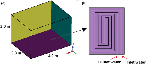
There was one existing study that analyzed the heating output and uniformity of surface temperature distribution, and created a realistic room model same as the full-scale experiment (Zheng et al. 2017), as shown in Figure 1. However, the total computational grid reached 3,014,151 including tetrahedral cells, hexahedral cells and mixed cells resulting in a certain burden of computer hardware.

Figure 1. Schematic diagram of the three-dimensional computational model: (a) isometric view of the simulation; (b) the pipe arrangement of the floor (Zheng et al. 2017).

Although the simplified two dimensional model can capture the distribution of surface temperature and calculate the system cooling capacity (Rhee, Olesen, and Kim 2017), the uniformly surface temperature and minimal surface temperature cannot be correctly evaluated (Xie et al. 2016), correspondingly, the condensation on radiant cooling surfaces cannot be effectively prevented (Xing et al. 2021). Therefore, to upgrade the computational efficiency and ensure the accuracy of calculated surface temperature distribution, the simplified three dimensional heat transfer model should be one important target of this study.

In recent year, the development of neural networks has attracted much attention, and artificial neural network (ANN) models have been widely used in many different studies. The neural network structure mimics the function of the human brain, which is characterized by nonlinear information processing (Ye and Kim 2018). At present, ANN has been used by many researchers to quickly predict radiant air conditioning system (Cao et al. 2022). Çolak et al. (2022) developed three unique ANN models to predict the radiative, convective and total heat transfer coefficient of floor surface of radiant floor heating system in real room. The results of numerical analysis show that the best prediction performance is Levenberg-Marquardt algorithm. This study is the forerunner of ANN for nanofluid floor heating systems. Acikgoz et al. (2022) combined the experiment with ANN to predict the heat transfer coefficient of the radiant cooling system and verified the accuracy of the established ANN model. This approach was the first to use experiment to obtain artificial neural network data. Ge et al. (2012) used neural network to predict the ceiling surface temperature, air dew point temperature and the best opening time of the ventilation system to prevent the condensation. Çolak et al. (2023) designed seven different ANN models to estimate the total heat transfer coefficient, radiative heat transfer coefficient, convective heat transfer coefficient and heat transfer rate. The ANN was found to be superior to well-known correlations in estimating experimental results. However, compared to the radiation ceiling systems (Nasruddin et al. 2019), there are limited studies on radiant floor system combined with neural network for prediction. Su et al. (2022) used ANN to predict the time and pre-dehumidification of radiant floor cooling system to prevent condensation. Lee et al. (2002) proposed the predictive control based on ANN for radiant floor cooling system, and the feasibility of the method is verified by experiments. These studies did not mention the performance of radiant floor, therefore, another important target of this study is to use ANN to rapidly predict the cooling capacity and minimum floor temperature, which can evaluate the cooling performance of the radiant floor.

Aiming at two important targets, a simplified three-dimensional model of a radiant cooling floor is established, and ANSYS Fluent 16.2 software is used to simulate the temperature environment of the floor structural layers. The total cooling capacity (Q_t) and minimum floor temperature (T_f,min) are taken as the parameters to evaluate the cooling performance, and different factors affecting the two indexes are considered as design variables. The backpropagation (BP) neural network adopts error back propagation learning algorithm, which is the most widely used prediction algorithm at present (Kim, Kim, and Srebric 2020). Therefore, based on the CFD simulation and BP neural network model, the influences of different design parameters on Q_t and T_f,min are analyzed. The neural network is found to quickly predict the values of Q_t and T_f,min, and the prediction program was established based on the trained neural network model. This study provides a novel and effective method by which to evaluate the cooling performance of radiant floors.

2. The simplified 3D geometric model

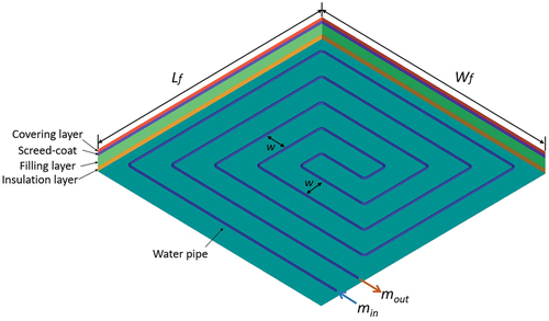
A schematic diagram of a typical radiant floor structure with counterflow water pipes is shown in Figure 2. Four structural layers including a cover layer, screed-coat, filling layer, and insulation layer are presented. The spacing between the pipes is uniformly arranged.

Figure 2. The schematic diagram of a typical radiant floor structure with counterflow water pipes.

For the assumption of a simplified counterflow layout, the following considerations are made to propose a simplified 3D counterflow pipe model, as shown in Figure 2.

1. The counterflow pipe and simplified counterflow pipe located in the filling layer have the same length.

2. The effect of the 90-degree bend of the pipe extremities on the resistance loss and heat transfer is neglected.

3. The spacing between the straight pipes is constant.

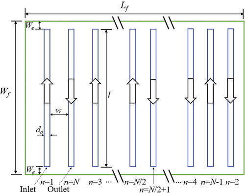
The simplified counterflow configuration is presented in Figure 3. The total pipe length for the original counterflow configuration is averagely divided into N pipe sections arranged in a floor surface area of L_f × W_f. An even number of pipes is alternately arranged from both sides to the center. Their sequence in naming follows the alphabetical order of n₁, n₂, n₃, … n_n/2, n_N/2 + 1, … , n_N-1, and n_N. The water temperature and velocity at each pipe row inlet are the same as those at the previous pipe row outlet. Note that the user-defined function compilation was used to obtain the mean water temperature of each pipe row outlet and then transfer it to the subsequent pipe row inlet. Each straight pipe has the same length l. The spacing between the pipes is w, and the distance between the pipe extremities and side walls of the floor is w_e, as determined by calculating the difference between the width of the floor and the pipe length. The inner and outer pipe diameters are d_i and d_o, respectively.

Figure 3. The top view of a simplified counterflow configuration with their dimensions and the pipes’ sequence.

An example of a simplified procedure is proposed according to a chamber experiment with an underfloor radiant cooling system (Karakoyun et al. 2020), as shown in Figure 4. The total area of the floor is L_f × W_f = 1.8 m × 1.8 m, and the spacing between the pipes is w = 0.12 m. A total pipe length of 23.8 m is obtained and divided into 14 sections with a length of l = 1.7 m for each pipe. Moreover, a distance of w_e = 0.05 m between the pipe extremities and side walls of the floor is calculated.

Figure 4. Two configurations of water flow pipes: (a) counterflow; (b) simplified counterflow. Blue sequence numbers indicate the inlet opening, and red sequence numbers indicate the outlet opening.

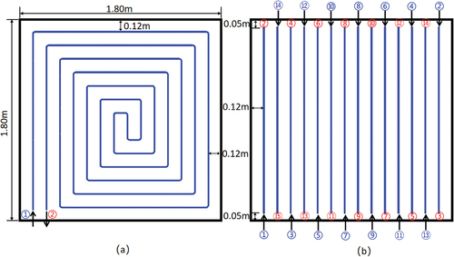
For the counterflow configuration, there is only one inlet and one outlet opening, while the simplified counterflow configuration has up to 14 inlet and 14 outlet openings. In the figure, the water temperature and velocity at outlet No. 1 are used as the boundary conditions of inlet No. 2. Therefore, in sequence, the water temperature and velocity at each pipe row inlet No. n are the same as those of the previous pipe row outlet n - 1.

Moreover, the following assumptions for the numerical simulation are considered.

1. Homogeneous, isotropic, and constant thermophysical properties of solids are assumed.

2. The contact thermal resistance between solids is disregarded.

3. The bottom and the side walls of the floor are considered adiabatic.

4. The physical parameters of the supplied chilling water are regarded as constant.

3. Numerical method

3.1. Description of simulation cases

This study considers the radiant floor structure with a cover layer thickness of 10–30 mm, a screed-coat thickness of 20 mm, a filling layer thickness of 40–60 mm, a pipe outer diameter of 16–25 mm, and an insulation layer thickness of 20 mm. A sectional diagram of a typical radiant floor structure is presented in Figure 5, where R20-w200-δ50/20/20 indicates that this multi-layer floor structure has an outer pipe diameter of 20 mm, a pipe spacing of 200 mm, and thicknesses of 50, 20, and 20 mm for the filling layer, screed-coat, and cover layer, respectively. Note that the insulation layer has a constant thickness (30 mm) in all simulation cases.

Figure 5. The sectional diagram of a typical radiant floor structure (R20-w200-δ50/20/20).

To compare the effects of different thermal conductivities on the cooling performance, five different thermal conductivities for the cover layer, filling layer, and pipe are defined, as shown in Table 2. The pipe considers d_i/d_o of 12/16, 16/20, and 20/25 mm, respectively, so the pipe thicknesses are respectively 2.0, 2.0, and 2.5 mm.

Table 2. The predefined thickness and thermal physical parameters of the floor structure.

Floor component (Inside to outside)	Thickness (mm)	Density (kg/m^3)	Thermal conductivity (W/m·K)	Specific heat capacity (J/kg·K)
Cover layer	10, 20, 30	2000	0.2, 0.5, 0.8, 1.1, 1.4	950
Screed-coat	20	1700	0.9	1000
Filling layer	40, 50, 60	1800	0.8, 1.0, 1.2, 1.4, 1.6	1000
Pipe	2, 2.5	1050	0.28, 0.33, 0.38, 0.43, 0.48	1000
Insulation	20	400	0.035	2000

Detailed descriptions of the pipe length design with different pipe spacings (0.15, 0.20, 0.25, and 0.30 m) are presented in Table 3. Note that the curvature in the 90-degree bend of the pipe extremities is more practically considered as 20 mm.

Table 3. The descriptions of the pipe length design with different pipe spacings.

Pipe spacing (m)	Distance to the side wall (m)	Total pipe length* (m)	Length per pipe (m)	Total sub-pipe number (-)
0.15	0.16	69.98	3.88	18
0.20	0.16	54.49	3.89	14
0.25	0.125	47.10	3.92	12
0.30	0.15	39.20	3.92	10

Note: * The curvature in the 90-degree bend of the pipe extremities is set as 20 mm.

Five floor surface area sizes, including 2 × 3, 3 × 3, 4 × 3, 5 × 3, and 6 × 3 m², are selected to evaluate the effect of the water flow path length on the floor cooling capacity. Table 4 presents the pipe length design with different floor areas when the pipe spacing is 0.20 m.

Table 4. The descriptions of the pipe length design with different floor areas when the pipe spacing is 0.20 m.

Floor surface area, Lf×Wf (m^2)	Total pipe length (m)	Length per pipe (m)
2 × 3	26.62	1.90
3 × 3	4.36	2.88
4 × 3	54.49	3.89
5 × 3	68.44	4.89
6 × 3	82.54	5.90

3.2. Numerical model

ANSYS Fluent 16.2 software was used for numerical simulation (ANSYS Inc 2014). The averaged Navier – Stokes equations including the continuity equation, momentum conservation equation, and energy conservation equation can respectively be expressed as follows (Dastbelaraki et al. 2018):

(1) $\frac{\mathrm{\partial \rho }}{\mathrm{\partial t}}+\frac{\mathrm{\partial }\left(\rho U_i\right)}{\mathrm{\partial }{x}_j}=0,$(1)

(2) $\frac{\mathrm{\partial }\left(\rho U_i\right)}{\mathrm{\partial }\mathit{t}}+\frac{\mathrm{\partial }\left(\rho U_i{U}_j\right)}{\mathrm{\partial }{x}_j}=-\frac{\mathrm{\partial }\mathit{p}}{\mathrm{\partial }{x}_i}+\frac{\mathrm{\partial }}{\mathrm{\partial }{x}_j}\left[{\mu }_{\mathit{eff}}\left(\frac{\mathrm{\partial }{U}_i}{\mathrm{\partial }{x}_j}+\frac{\mathrm{\partial }{U}_j}{\mathrm{\partial }{x}_i}-\frac{2}{3}{\delta }_{\mathit{ij}}\frac{U_i}{x_i}\right)\right]+\frac{\mathrm{\partial }}{\mathrm{\partial }{x}_j}\left(-\mathit{\rho }\overline{u_i^{\prime }{u}_j^{\prime }}\right),$(2)

(3) $\frac{\partial \left(\mathit{\rho E}\right)}{\partial \mathit{t}}+\frac{\partial }{\partial x_i}\left[U_i\left(\mathit{\rho E}+\mathit{p}\right)\right]=\frac{\partial }{\partial x_j}\left(k_{\mathit{eff}}\frac{\partial \mathit{T}}{\partial x_i}+U_i\left(\frac{\partial U_i}{\partial x_j}+\frac{\partial U_j}{\partial x_i}-\frac{2}{3}{\delta }_{\mathit{ij}}\frac{U_i}{x_i}\right)\right)+S_h$(3)

where p is the static pressure, μ_eff is the eddy viscosity, k_eff is the effective conductivity, $-\mathit{\rho }\overline{u_i^{\prime }{u}_j^{\prime }}$ is the Reynolds stress, and S_h is the source term. E is the total energy, which is given as

(4) $\mathit{E}=\mathit{h}-\frac{p}{\rho }+\frac{U_i}{2},$(4)

where h is the sensible enthalpy.

The shear-stress transport (SST) k-ω turbulence model was used in this study (Menter 1994). The model combines the advantages of the k-ω model in the near-wall region and the k-ω model in the far-field. The semi-implicit method for pressure-linked equations (SIMPLE) was used for pressure-velocity coupling. The numerical simulations were based on the finite volume method. The conjugate heat transfer was used to model the heat transfer between the fluid medium and the pipe solid surface. The least-squares cell-based method was used for the gradient. Second-order discretization was specified for other terms. Convergence was achieved when the residuals were less than 10⁻⁶ for the energy term and 10⁻⁴ for all other variables.

3.3. Calculation of heat flux

The total heat exchange between the radiant floor surface and the indoor environment is constituted by the radiation heat flux (Q_r, W/m²) and convective heat flux (Q_c, W/m²). Therefore, the total cooling capacity (Q_t, W/m²) can be expressed as follows (ASHRAE 2012):

(5) $Q_t=Q_r+Q_c,$(5)

(6) $Q_r=\mathit{\epsilon \sigma }\left(\mathit{AUS}{T}^{\ast 4}-T_f^{\ast 4}\right),$(6)

(7) $Q_c=h_c\left(T_{\mathit{air}}-T_f\right),$(7)

where ε is the surface emissivity, σ is the Stefan-Boltzmann constant, 5.8 × 10⁻⁸ W/(m²·K⁴); h_r is the radiative heat transfer coefficient, W/(m².K); h_c is the convective heat transfer coefficient, W/(m².K); AUST^* is the area-weighted average uncooled temperature, K; AUST is the area-weighted average uncooled temperature, °C; T_air is the indoor air temperature, °C; T_f* is the mean radiant floor surface temperature, K; and T_f is the mean radiant floor surface temperature, °C.

According to ASHRAE standard (ASHRAE 2012), when the radiant floor cooling system accounts for the majority of heat exchange between the radiant floor surface and the indoor environment, therefore, the Eqs. (6)(6) $Q_r=\mathit{\epsilon \sigma }\left(\mathit{AUS}{T}^{\ast 4}-T_f^{\ast 4}\right),$(6) and (7(7) $Q_c=h_c\left(T_{\mathit{air}}-T_f\right),$(7) ) can be changed as the following ones that can respectively estimate the radiation heat flux and the convective heat flux from the cold floor surface.

(8) $Q_r=5.0\times {10}^{-8}\left[{\left(\mathit{AUST}+273\right)}^4-{\left(T_f+273\right)}^4\right],$(8)

(9) $Q_c=0.87{\left(T_f-T_{\mathit{air}}\right)}^{1.25},$(9)

For the convective heat flux, Eq. (9)(9) $Q_c=0.87{\left(T_f-T_{\mathit{air}}\right)}^{1.25},$(9) mainly represents the natural convection effect, and the forced convection effect of mechanical ventilation is not included in this study.

3.4. Boundary conditions

The simulation was conducted in a steady state. The insulation layer was set as an adiabatic boundary, and its thickness was 30 mm for all the cases. The settings of the thermal physical parameter conditions for the screed-coat, cover, and filling layers are shown in Table 2. The different layers’ materials, including their specific heat and thermal conductivity, were considered in this study. The inlet of the water pipe was set as the velocity-inlet condition, and the variation of the supply water temperature and the water mass flow rate was taken into account, as shown in Table 5. The turbulence intensity (I) and turbulence length scale (l) were set according to the equations below (EI-Behery and Hamed 2011).

Table 5. The mean water supply temperature and mass flow rate.

Parameters	Value
Supply water temperature, Tsup (°C)	16, 17, 18, 19, 20
Water mass flow rate, mw (kg/s)	0.03, 0.06, 0.09, 0.12

(10) $\mathit{I}=0.16{\left(\mathit{R}{\mathit{e}}_{\mathit{DH}}\right)}^{-1/8}$(10)

(11) $\mathit{l}=\frac{0.07\mathit{L}}{{C_{\mu }}^{3/4}}$(11)

Re_DH is the Reynolds number with the characteristic length scale using the hydraulic diameter; L is the characteristic length, C_μ is the constant with value of 0.09 in the k-ω turbulence model. The outlet of the water pipe was set as the outflow condition. The water pipe surface was no-slip, and the water was set as an incompressible fluid. The floor was set as the mixed thermal boundary condition, and the details are reported in Table 6.

Table 6. The mixed thermal boundary conditions for the floor surface (Ren et al. 2022; Zhu et al. 2022.).

AUST	External emissivity ε	Indoor air temperature Tair	Heat transfer coefficient hc
29 °C	0.9	26.5 °C	0.87 W/(m^2·K)

3.5. Grid independence analysis

Hybrid meshes were used, including triangular meshes around the heating pipe and quadrilateral meshes in other solid zones and the indoor air zone. The grid diagram is exhibited in Figure 6. To test the independence of the grid, coarse, medium, and fine grids with 198,676, 291,772, and 344,672 computing units, respectively, were selected to study the grid independence. The air temperature at a height of 1.1 m and the floor surface temperature were compared, as shown in Table 7. With the increase of the computational units from 198,676 (coarse grids) to 291,772 (medium grids), the relative differences of the floor surface temperature and air temperature at a height of 1.1 m were respectively 0.73% and 0.94%. With the increase of the computational units from 291,772 (medium grids) to 344,672 (fine grids), the relative differences of the floor surface temperature and air temperature at a height of 1.1 m were respectively 0.26% and 0.51%, which are smaller. Therefore, medium grids were selected for subsequent simulation.

Figure 6. The grid distribution in the sectional diagram.

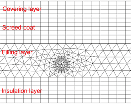
Table 7. The grid independence analysis.

	Pipe element size/Heat source grid size	Total number of grids	ΔT (Floor surface temperature)	ΔT (Air temperature at a height of 1.1 m)
Coarse mesh	1.5 mm/15 m	198,676	-	-
Medium mesh	1 mm/10 mm	291,772	0.73 %	0.94 %
Fine mesh	.8 mm/8 mm	344,672	0.26 %	0.51 %

Note: The boundary layers around the heat source, the grid numbers (≥8) of the inlet and outlet, and the grid number (≥3) for each component in the multilayer structures were kept constant for each case. ΔT means the temperature relative difference.

3.6. Validation of the CFD simplified counterflow model

To verify the accuracy of the simplified counterflow model constructed in this study, the simulated data were compared with existing experimental data (Acikgoz et al. 2019). The schematic diagram of the laboratory used by Acikgoz et al. is shown in Figure 7(a). Nine measurement points were evenly distributed on the floor surface. Figure 7(b) shows the pipe arrangement in the test room. Figure 8 illustrates the comparison between experiment data and CFD simulation results regarding the mean return water temperature (T_w), the mean floor temperature (T_f), and the total heat transfer flux (Q_t, W/m²). As shown in Figure 8(a,b), all the values of T_f and T_w are within the range of ± 5%. Moreover, 88% of the values of Q_t are in the ± 5% range, as shown in Figure 8(c). As shown in Table 8, the average relative errors between the experimental and simulation results for the three parameters were respectively found to be 0.07%, 1.24%, and 2.21%, which are within the allowable error range. The model established in this study was therefore verified via comparison with the experimental results (Acikgoz et al. 2019). The good consistency demonstrates that the accuracy of the model is sufficient for further study.

Figure 7. The schematic diagram of the laboratory: (a) the layout of measurement points; (b) the pipe arrangement in the test room (Acikgoz et al. 2019).

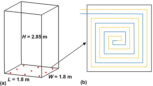
Figure 8. The CFD validation via comparison with the experiment: (a) mean return water temperature; (b) mean floor temperature; (c) total heat transfer flux.

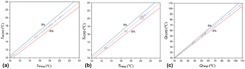
Table 8. The error analysis of the numerical data compared with the experimental data.

	Tw (^oC)	Tf (^oC)	Qt (W/m^2)
Maximum relative error	0.23%	3.56%	5.54%
Average relative error	0.07%	1.24%	2.21%

4. BP neural network

As the most widely used neural network learning algorithm (Hsu 2015), the BP neural network is a multilayer feed-forward neural network, the algorithm of which propagates backward according to the error during training (Ye and Kim 2018). In this study, three neural layers were used, including an input layer, a hidden layer, and an output layer. The sigmoid function was selected as the activation equation. Figure 9 presents the structure of the BP neural network and the sigmoid function.

Figure 9. The structure of the BP neural network (Zhang et al. 2020).

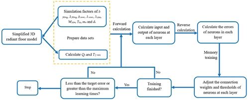
There are multiple influencing factors of T_f,min and Q_t, but there is no linear function to express the relationship between T_f,min (or Q_t) and their influencing factors. Therefore, in the BP neural network model, nine influencing factors, namely the filling thickness (δ_filling), filling conductive heat transfer coefficient (λ_filling), cover thickness (δ_cover), cover conductive heat transfer coefficient (λ_cover), pipe conductive heat transfer coefficient (λ_pipe), pipe width (W_pipe), supply water temperature (T_sp), water mass flow (m_w), and pipe diameter (d_o), were used as input values. Moreover, T_f,min and Q_t were used as output values for training, and the mapping relationship between the input and output was obtained. Figure 10 describes the learning and training process of the BP neural network.

Figure 10. The flow chart of the BP algorithm.

Two statistical indexes are adopted for evaluation in this study, namely the root-mean-square error (RMSE) and the coefficient of determination (R²), as respectively given by the following equations (Nasruddin et al. 2019):

(12) $\mathit{RMSE}=\sqrt{\frac{1}{n}{\sum }_i{\left|{\hat{y}}_{\mathit{i}}-y_i\right|}^2},$(12)

(13) $R^2=1-\frac{{\sum }_{i=0}^n{\left({\hat{y}}_{\mathit{i}}-{\bar{y}}_{\mathit{i}}\right)}^2}{{\sum }_{i=0}^n{\left(y_i-{\bar{y}}_{\mathit{i}}\right)}^2},$(13)

where ${\hat{y}}_{\mathit{i}}$ is the predicted value and y_i is the simulated value.

5. Results

5.1. CFD simulation results

5.1.1. Floor temperature distribution

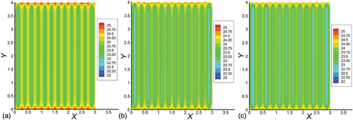
Figure 11 exhibits the floor temperature cloud at distances Y = 0.8, 1.6, 2.4, and 3.2 m from the pipe inlet. The shape of the temperature field is roughly a group of concentric circles centered on the pipe. The temperature changes sharply near the pipe, and the farther away from the pipe, the more slowly the temperature changes. Compared with the vertical Z-direction, there is no significant temperature variation along the Y-direction of the pipe length. Figure 12 shows the temperature distribution of the pipe at different values of d_o, from which can be seen that the water flow temperature in the pipe gradually decreases with the increase of d_o. Furthermore, the variation of the water temperature is more drastic at the inlet and outlet, and is not obvious at greater distances from the inlet and outlet.

Figure 11. The distribution diagram of the floor temperature (°C) at different sections.

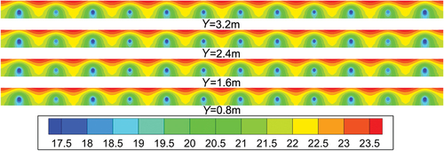
Figure 12. The distribution diagram of the floor temperature (°C) at different values of d_o: (a) d_o = 16 mm; (b) d_o = 20 mm; (c) d_o = 25 mm.

5.1.2. Total cooling capacity

Table 9 describes the effect of the water supply with and without pipe wall thickness on T_w, T_f, and Q_t. When d_i/d_o = 12/16 mm, the pipe wall thickness is 2 mm. As can be seen from the table, the pipe wall thickness has a certain influence on T_w, T_f, and Q_t. When the pipe with wall thickness is considered, T_w, T_f, and Q_t are respectively 19.10 °C, 23.82 °C, and 34.26 W/m². Compared with the pipe without considering the wall thickness, the relative errors are respectively 0.38%, 1.33%, and 6.42%. When d_i/d_o = 20/25 mm, the pipe wall thickness is 2.5 mm, and T_w, T_f, and Q_t exhibit the same trends. The relative errors between these parameters for the pipe with and without considering the wall thickness are respectively 0.35%, 1.28%, and 5.7%. It can be concluded that the cooling effect of the pipe without considering the wall thickness is better than that of the pipe for which the wall thickness is considered. Furthermore, when the pipe wall thickness is 2 mm and d_i/d_o varies from 12/16 to 16/20 mm, Q_t varies from 34.26 to 34.93 W/m², a variation of 1.91%.

Table 9. The effect of the water supply with and without the pipe wall thickness.

		Tw (^oC)	Tf (^oC)	Qt (W/m^2)
di/do = 12/16 mm	With	19.10	23.82	34.26
	Without	19.18	23.50	36.46
	Relative error (%)	0.38	1.33	6.42
di/do = 16/20 mm	With	19.13	23.72	34.93
	Without	19.19	23.46	36.75
	Relative error (%)	0.28	1.11	5.23
di/do = 20/25 mm	With	19.19	23.51	36.43
	Without	19.26	23.21	38.50
	Relative error (%)	0.35	1.28	5.70

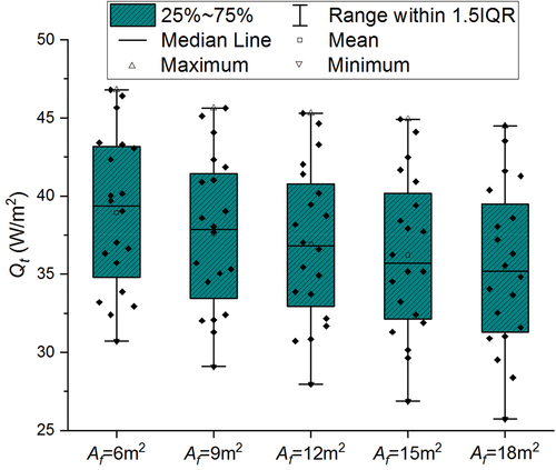
Therefore, increasing the pipe diameter can also enhance the cooling effect, but decreasing the pipe wall thickness has a significant effect. Figure 13 shows the distribution of Q_t for different floor surface areas (A_f). With the increase of the A_f, i.e., with the gradual increase of the length of the pipe, Q_t gradually decreases. When A_f = 6 m², Q_t varies from 33.2 to 43.3 W/m², and when A_f = 18 m², Q_t varies from 31.5 to 36.4 W/m²; thus, the variation range of Q_t is gradually decreasing.

Figure 13. The distribution of Q_t for different floor surface areas.

5.2. Model validation and prediction program

5.2.1. Validation of the prediction model

Note that 80% of the data were randomly selected for neural network training, and the remaining data were used for validation. The number of iterations of the neural network was 1000, and the learning rate was 0.05. After repeated training, a better model was obtained. Figure 14 exhibits the validation results of the prediction model. It can be seen from Figure 14(a,c) that the predicted and simulated data exhibit good consistency. Figure 14(b) shows that the R² and RMSE values for the total cooling capacity were respectively 0.9117 and 1.5849. By comparing the differences between the predicted results and the simulated original data of the Q_t, the maximum error in the validation of Q_t was found to be 10 W/m², and the error in other validation samples was smaller.

Figure 14. The validation results of the simulated and predicted data: (a, b) the comparison results of the total cooling capacity; (c, d) the comparison results of the minimum temperature.

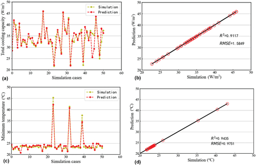
Figure 14d shows that the R² and RMSE values for the T_f,min were respectively 0.9435 and 0.9751. By comparing the differences between the predicted results and the simulated original data of the T_f,min, the maximum error in the validation of T_f,min was found to be 2.5 °C, and the error in the other validation samples was smaller. These findings indicate that the prediction model established in this study can well reflect the relationship between the outputs and inputs. Therefore, the model can be saved for the later direct invocation of predictions. In future practical applications, the BP neural network can be used for the accurate estimation of Q_t and T_f,min according to the operating parameters of the floor environment.

5.2.2. Establishment of prediction program

As shown in Figure 15, the prediction program was established based on the trained BP neural network, which can quickly predict Q_t and T_f,min. Figure 15(a) exhibits the interface of the single prediction. The case with specific value of δ_cover, λ_cover, δ_filling, λ_filling, T_sp, m_w, δ_pipe, λ_pipe, W_pipe and d_o were taken as an example to input into the interface. The difference of Q_t between predicted value and simulated value was 1.05 W/m², and the difference of T_f,min was 1.14 °C, which were within the permissible range. Figure 15(b) exhibits the interface of the batch prediction, which can read a large amount of data for prediction. Figure 15(c) is the image display interface of predicted Q_t and T_f,min. The steps for application of this program are as follows:

Figure 15. Interfaces of the prediction program: (a) single predict; (b) batch predict; (c) image display.

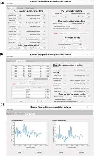
Step1: when the single predict interface is opened, enter the corresponding value in the parameter input box, and then click predict button to predict Q_t and T_f,min. Finally, click reset button to return each parameter to 0.

Step2: when the batch predict interface is opened, click the import data button to locate data file and open it. Subsequently, click predict button to predict the Q_t and T_f,min in batches, and click the download button to download the predicted values to the appropriate path.

Step3: when the image display interface is opened, click the display button to show an image of the predicted values, and click the download button to download the image.

5.3. BP prediction results

5.3.1. Total cooling capacity

Figure 16 shows the 3D diagrams of the variation trends of Q_t. Figure 16(a,b) present the effects of the cover and filling floor structural layers on Q_t, respectively. The thickness and heat transfer coefficients of the two structural layers are considered. It can be seen from the figures that with the increase of δ_cover and δ_filling, Q_t decreases. When λ_cover = 0.5 W/(m·K), with the increase of δ_cover from 0.005 to 0.05 m, Q_t decreases from 33.95 to 30.97 W/m², a variation of 8.77%. When λ_filling = 1.0 W/(m·K), with the increase of δ_filling from 0.02 to 0.065 m, Q_t decreases from 38.46 to 30.19 W/m², a variation of 21.5%. The reason for this phenomenon is that with the increase of δ_cover and δ_filling, the floor surface temperature decreases slowly. The greater the thickness, the higher the temperature of the floor surface. According to Eq. (12)(12) $\mathit{RMSE}=\sqrt{\frac{1}{n}{\sum }_i{\left|{\hat{y}}_{\mathit{i}}-y_i\right|}^2},$(12) , with the increase of the floor surface temperature, the difference decreases, and Q_t decreases.

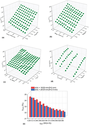
Figure 16. The 3D diagrams of the variation trends of Q_t for different influencing factors: (a) the effects of δ_cover and λ_cover; (b) the effects of δ_filling and λ_filling; (c) the effects of T_sp and m_w; (d) the effects of W_pip and d_o; (e) the effect of λ_pipe.

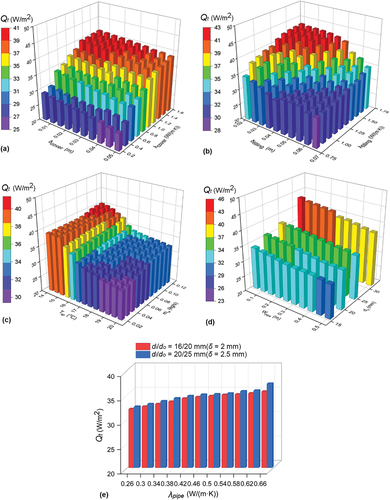
However, with the increase of λ_cover and λ_filling, Q_t increases. When δ_cover = 0.03 m, with the increase of λ_cover from 0.2 to 1.55 W/(m·K), Q_t increases from 27.58 to 39.72 W/m². When δ_filling = 0.03 m, with the increase of λ_filling from 0.8 to 1.7 W/(m·K), Q_t increases from 32.52 to 42.49 W/m². The reason for this phenomenon is that with the increase of λ_cover and λ_filling, the floor surface temperature decreases rapidly. The greater the heat transfer coefficient, the lower the temperature of the floor surface. According to Eq. (12)(12) $\mathit{RMSE}=\sqrt{\frac{1}{n}{\sum }_i{\left|{\hat{y}}_{\mathit{i}}-y_i\right|}^2},$(12) , the temperature difference increases, and Q_t increases.

Figure 16(c) shows the effects of T_sp and m_w on Q_t. With the increase of T_sp, Q_t decreases, and with the increase of m_w, Q_t increases. With the variation of T_sp from 14 to 20 °C, Q_t varies by 24.3%. With the variation of m_w from 0.02 to 0.12 kg/s, Q_t varies by 7.39%. Figures 16(d) and 15(e) present the effects of the water pipe features W_pipe, λ_pipe, and d_o on Q_t. It can be seen that Q_t decreases with the increase of W_pipe. Taking d_o = 20 mm as an example, with the increase of W_pipe from 0.05 to 0.5 m, Q_t decreases from 35.75 to 32.91 W/m². With the increase of λ_pipe and d_o, Q_t exhibits an increasing trend. Taking d_i/d_o = 16/20 mm and W_pipe = 1.3 as examples, with the increase of λ_pipe from 0.026 to 0.66 W/(m·K), and with the increase of d_o from 16 to 32 mm, Q_t respectively increases by 10.05% and 19.89%. This is because with the increase of λ_pipe and d_o, the floor temperature drops rapidly, and the temperature difference increases. With the increase of W_pipe, Q_t exhibits the opposite effect.

5.3.2. Minimum floor temperature

Figure 17 presents the 3D diagrams of the variation trends of T_f,min. Figure 17(a) shows the effects of λ_cover and δ_cover on T_f,min. With the increase of λ_cover, T_f,min increases. When λ_cover = 0.35 W/(m·K), with the increase of δ_cover from 0.005 to 0.05 m, T_f,min increases from 20.68 to 23.23 °C, a variation of 10.97 %. When δ_cover = 0.035 m, with the increase of λ_cover from 0.2 to 1.55 W/(m·K), T_f,min decreases from 22.49 to 21.54 °C. Figure 17(b) shows the effects of λ_filling and δ_filling on T_f,min, from which it can be seen that the trends of the influences of λ_filling and δ_filling on T_f,min are consistent with the trends shown in Figure 17(a). With the increase of the thickness of the cover and filling layers, the temperature transfer becomes slow, and T_f,min increases gradually. Conversely, with the increase of the heat transfer coefficient of the cover and filling layers, the temperature transfer becomes rapid, and T_f,min decreases gradually.

Figure 17. The 3D diagrams of the variation trends of T_f,min for different influencing factors: (a) the effects of δ_cover and λ_cover; (b) the effects of δ_filling and λ_filling; (c) the effects of T_sp and m_w; (d) the effects of W_pip and d_o; (e) the effect of λ_pipe.

Figure 17c shows the effects of T_sp and m_w on T_f,min. With the increase of T_sp, T_f,min increases. When m_w = 0.03 kg/s, with the increase of T_sp from 14 to 20 °C, T_f,min increases from 22.25 to 24.02 °C, a variation of 7.37%. However, with the increase of m_w, T_f,min exhibits a decreasing trend. Figure 17(d,e) present the effects of the water pipe features W_pipe, λ_pipe, and d_o on T_f,min. With the increase of λ_pipe and d_o, the temperature transfer becomes rapid, and T_f,min decreases gradually, which will enhance the cooling effect. With the increase of λ_pipe from 0.26 to 0.66 W/(m·K), T_f,min decreases from 24.34 to 22.02 °C. With the increase of W_pipe, the temperature transfer becomes slow, and T_f,min increases gradually, which will weaken the cooling effect. When d_o = 25 mm, with the increase of W_pipe from 0.15 to 0.5 m, T_f,min increases from 21.52 to 22.86 °C, a variation of 5.8%. When W_pipe = 0.35 m, with the increase of d_o from 16 to 32 mm, T_f,min decreases from 23.16 to 22.08 °C.

6. Discussion

In this study, an artificial intelligence method was proposed to rapidly predict the values of Q_t and T_f,min. The advantages of this study compared to similar studies are the simplification of the 3D model of a radiant floor, which accelerates the simulation, as well as the combination of CFD with a neural network model. However, there are some limitations, e.g., the different forms of the pipeline layout and the phase-change materials (PCM) were not sufficiently considered. Compared with traditional concrete, PCM has a higher latent heat storage capacity which can achieve significant energy saving and improve the thermal comfort of occupants in lightweight buildings (Mohammadzadeh and Kavgic 2020).

Furthermore, solar heat gain was not considered while it was an important factor to influencing the cooling load of a building (Zhao et al. 2022). The radiant floor cooling capacity is related to the solar radiation distribution (Cui et al. 2023). The locality, fluidity and intensity variation were shown when the sunlight on the floor surface, which has an important impact on the floor surface temperature (Tang et al. 2018). More comprehensive factors will be considered in the future studies.

7. Conclusion

CFD was used to generate a database based on a simplified 3D radiant floor structure, and the BP neural network was used to predict the Q_t and T_f,min. Moreover, a prediction program was established based on the trained BP neural network. This study provides an artificial intelligence method for the rapid prediction of Q_t and T_f,min. The main conclusions are as follows.

1. The simulation results showed that the cooling effect of the pipe without considering the wall thickness is better than that of the pipe for which the wall thickness is considered. Additionally, with the increase of the A_f, i.e., with the gradual increase of the length of the pipe, Q_t gradually decreases.

2. The data predicted by the established prediction model based on BP neural network were in good agreement with the CFD simulated data. The R² values of Q_t and T_f,min were respectively 0.9117 and 0.9751, and the RMSE values were respectively 0.9751 and 1.5849. Besides, the prediction program established based on the trained BP neural network could quickly predict Q_t and T_f,min.

3. The prediction results showed that with the increase of the thickness of the floor structural layers, T_f,min increase and Q_t increase gradually. However, with the increase of the heat transfer coefficient of the floor structural layers, the cooling effect is enhanced. With the increase of δ_cover and δ_filling, T_f,min respectively increases by 10.97% and 11.01%. With the increase of λ_cover and λ_filling, Q_t respectively increases by 30.56% and 23.46%.

4. Regarding the water pipe characteristics, with the increase of d_o and λ_pipe, T_f,min decreases and Q_t increases; thus, the cooling capacity is enhanced. With the increase of W_pipe, the cooling capacity is weakened. Furthermore, with the decrease of T_sp and the increase of m_w, Q_t increases gradually and T_f,min decreases gradually.

Disclosure statement

No potential conflict of interest was reported by the authors.

Correction Statement

This article was originally published with errors, which have now been corrected in the online version. Please see Correction (https://doi.org/10.1080/13467581.2023.2251335).

Additional information

Funding

This work was funded by Natural Science Foundation of Shandong Province [ZR2021ME199, ZR2020ME211], and the Support Plan for Outstanding Youth Innovation Team in Colleges and Universities of Shandong Province [2019KJG005]. This work acknowledges the support of the Plan of Introduction and Cultivation for Young Innovative Talents in Colleges and Universities of Shandong Province.

Notes on contributors

Jiying Liu

Jiying Liu is a professor of Shandong Jianzhu University, Jinan, China. He is engaged in urban microclimate and human health, energy-saving and optimization of radiation air conditioning systems, and optimization of regional energy systems.

Meng Su

Meng Su is graduating from Shandong Jianzhu University, Jinan, China. She obtained her Master's degree in Engineering in 2023. Her research interest is radiant floor cooling system and computational fluid dynamics.

Moon Keun Kim

Moon Keun Kim is an associate professor of Oslo Metropolitan University, Oslo, Norway. He is interested in research of ventilation and air quality, building energy efficiency and radiant cooling system.

Shoujie Song

Shoujie Song is a senior engineer of Shandong Jianzhu University, Jinan, China. His major research field is the radiant floor cooling and heating system and building energy-saving technology.

References

- Acikgoz, O., A. B. Çolak, M. Camci, Y. Karakoyun, and A. S. Dalkilic. 2022. “Machine Learning Approach to Predict the Heat Transfer Coefficients Pertaining to a Radiant Cooling System Coupled with Mixed and Forced Convection.” International Journal of Thermal Sciences 178:107624. https://doi.org/10.1016/j.ijthermalsci.2022.107624.
- Acikgoz, O., Y. Karakoyun, Z. Yumurtacı, N. Dukhan, and A. S. Dalkılıç. 2019. “Realistic Experimental Heat Transfer Characteristics of Radiant Floor Heating Using Sidewalls as Heat Sinks.” Energy and Buildings 183:515–526. https://doi.org/10.1016/j.enbuild.2018.11.022.
- Almeida, R. M. S. F., R. D. S. Vicente, A. Ventura-Gouveia, A. Figueiredo, F. Rebelo, E. Roque, and V. M. Ferreira. 2022. “Experimental and Numerical Simulation of a Radiant Floor System: The Impact of Different Screed Mortars and Floor Finishings.” Materials 15 (3): 1015. https://doi.org/10.3390/ma15031015.
- Amini, M., R. Maddahian, and S. Saemi. 2020. “Numerical Investigation of a New Method to Control the Condensation Problem in Ceiling Radiant Cooling Panels.” Journal of Building Engineering 32:101707. https://doi.org/10.1016/j.jobe.2020.101707.
- ANSYS Inc. 2014. ANSYS FLUENT Theory Guide, Release 16.1. Canonsburg, PA: ANSYS Inc press.
- ASHRAE. 2012. HVAC Systems and Equipment, Chapter 6: Panel Heating and Cooling. Atlanta, GA: American Society of Heating Air-Conditioning and Refrigeration Engineers.
- Benzar, B.-E., M. Park, H.-S. Lee, I. Yoon, and J. Cho. 2020. “Determining Retrofit Technologies for Building Energy Performance.” Journal of Asian Architecture and Building Engineering 19 (4): 367–383. https://doi.org/10.1080/13467581.2020.1748037.
- Cao, S., S. Zhou, J. Liu, X. Liu, and Y. Zhou. 2022. “Wood Classification Study Based on Thermal Physical Parameters with Intelligent Method of Artificial Neural Networks.” BioResources 17 (1): 1187–1204. https://doi.org/10.15376/biores.17.1.1187-1204.
- Cholewa, T., M. Rosiński, Z. Spik, M. R. Dudzińska, and A. Siuta-Olcha. 2013. “On the Heat Transfer Coefficients Between Heated/Cooled Radiant Floor and Room.” Energy and Buildings 66:599–606. https://doi.org/10.1016/j.enbuild.2013.07.065.
- Çolak, A. B., O. Acikgoz, Y. K. Karakoyun, A. Koca, and A. S. Dalkılıç. 2023. “Experimental and Numerical Investigations on the Heat Transfer Characteristics of a Real-Sized Radiant Cooled Wall System Supported by Machine Learning.” International Journal of Thermal Sciences 191:108355. https://doi.org/10.1016/j.ijthermalsci.2023.108355.
- Çolak, A. B., Y. K. Karakoyun, O. Acikgoz, Z. Yumurtaci, and A. S. Dalkılıç. 2022. “A Numerical Study Aimed at Finding Optimal Artificial Neural Network Model Covering Experimentally Obtained Heat Transfer Characteristics of Hydronic Underfloor Radiant Heating Systems Running Various Nanofluids.” Heat Transfer Research 53 (5): 51–71. https://doi.org/10.1615/HeatTransRes.2022041668.
- Cui, M., J. Liu, M. K. Kim, and X. Wu. 2023. “Application Potential Analysis of Different Control Strategies for Radiant Floor Cooling Systems in Office Buildings in Different Climate Zones of China.” Energy and Buildings 282:112772. https://doi.org/10.1016/j.enbuild.2023.112772.
- Dastbelaraki, A. H., M. Yaghoubi, M. M. Tavakol, and A. Rahmatmand. 2018. “Numerical Analysis of Convection Heat Transfer from an Array of Perforated Fins Using the Reynolds Averaged Navier–Stokes Equations and Large-Eddy Simulation Method.” Applied Mathematical Modelling 63:660–687. https://doi.org/10.1016/j.apm.2018.06.005.
- Duarte, C. C., and N. D. Cortiços. 2022. “The Energy Efficiency Post-COVID-19 in China’s Office Buildings.” Clean Technologies 4 (1): 174–233. https://doi.org/10.3390/cleantechnol4010012.
- EI-Behery, S. M., and M. H. Hamed. 2011. “A Comparative Study of Turbulence Models Performance for Separating Flow in a Planar Asymmetric Diffuse.” Computers and Fluids 44 (1): 248–257. https://doi.org/10.1016/j.compfluid.2011.01.009.
- Feng, J., S. Schiavon, and F. Bauman. 2016. “New Method for the Design of Radiant Floor Cooling Systems with Solar Radiation.” Energy and Buildings 125:9–18. https://doi.org/10.1016/j.enbuild.2016.04.048.
- Fernández-Hernández, F., A. Fernández-Gutiérrez, J. J. Martínez-Almansa, C. Del Pino, and L. Parras. 2020. “Flow Patterns and Heat Transfer Coefficients Using a Rotational Diffuser Coupled with a Radiant Floor Cooling.” Applied Thermal Engineering 168:114827. https://doi.org/10.1016/j.applthermaleng.2019.114827.
- Ge, G., F. Xiao, and S. Wang. 2012. “Neural Network Based Prediction Method for Preventing Condensation in Chilled Ceiling Systems.” Energy and Buildings 45:290–298. https://doi.org/10.1016/j.enbuild.2011.11.017.
- Gu, X., M. Cheng, X. Zhang, Z. Qi, J. Liu, and Z. Li. 2021. “Performance Analysis of a Hybrid Non-Centralized Radiant Floor Cooling System in Hot and Humid Regions.” Case Studies in Thermal Engineering 28:101645. https://doi.org/10.1016/j.csite.2021.101645.
- Hsu, D. 2015. “Comparison of Integrated Clustering Methods for Accurate and Stable Prediction of Building Energy Consumption Data.” Applied Energy 160:153–163. https://doi.org/10.1016/j.apenergy.2015.08.126.
- Jin, Z., Y. Zheng, and Y. Zhang. 2022. “A Novel Method for Building Air Conditioning Energy Saving Potential Pre-Estimation Based on Thermodynamic Perfection Index for Space Cooling.” Journal of Asian Architecture and Building Engineering 22 (4): 1–17. https://doi.org/10.1080/13467581.2022.2109645.
- Karakoyun, Y., O. Acikgoz, Z. Yumurtacı, and A. S. Dalkilic. 2020. “An Experimental Investigation on Heat Transfer Characteristics Arising Over an Underfloor Cooling System Exposed to Different Radiant Heating Loads Through Walls.” Applied Thermal Engineering 164:114517. https://doi.org/10.1016/j.applthermaleng.2019.114517.
- Khatri, R., V. R. Khare, and H. Kumar. 2020. “Spatial Distribution of Air Temperature and Air Flow Analysis in Radiant Cooling System Using CFD Technique.” Energy Reports 6:268–275. https://doi.org/10.1016/j.egyr.2019.11.073.
- Kim, M. K., Y.-S. Kim, and J. Srebric. 2020. “Impact of Correlation of Plug Load Data, Occupancy Rates and Local Weather Conditions on Electricity Consumption in a Building Using Four Back-Propagation Neural Network Models.” Sustainable Cities and Society 62:102321. https://doi.org/10.1016/j.scs.2020.102321.
- Kim, M. K., J. Liu, and S.-J. Cao. 2018. “Energy Analysis of a Hybrid Radiant Cooling System Under Hot and Humid Climates: A Case Study at Shanghai in China.” Building and Environment 137:208–214. https://doi.org/10.1016/j.buildenv.2018.04.006.
- Krusaa, M. R., and C. A. Hviid. 2022. “Numerical Feasibility Study of Self-Regulating Radiant Ceiling in Combination with Diffuse Ceiling Ventilation.” Energies 15 (4): 1319. https://doi.org/10.3390/en15041319.
- Lee, J.-Y., M.-S. Yeo, and K.-W. Kim. 2002. “Predictive Control of the Radiant Floor Heating System in Apartment Buildings.” Journal of Asian Architecture and Building Engineering 1 (1): 105–112. https://doi.org/10.3130/jaabe.1.105.
- Li, Q.-Q., C. Chen, Y. Zhang, J. Lin, and H.-S. Ling. 2014. “Simplified Thermal Calculation Method for Floor Structure in Radiant Floor Cooling System.” Energy and Buildings 74:182–190. https://doi.org/10.1016/j.enbuild.2014.01.032.
- Liu, J., D. A. Dalgo, S. Zhu, H. Li, L. Zhang, and J. Srebric. 2019. “Performance Analysis of a Ductless Personalized Ventilation Combined with Radiant Floor Cooling System and Displacement Ventilation.” Building Simulation 12 (5): 905–919. https://doi.org/10.1007/s12273-019-0521-9.
- Liu, J., M. K. Kim, and J. Srebric. 2022. “Numerical Analysis of Cooling Potential and Indoor Thermal Comfort with a Novel Hybrid Radiant Cooling System in Hot and Humid Climates.” Indoor and Built Environment 31 (4): 929–943. https://doi.org/10.1177/1420326X211040853.
- Liu, J., Z. Li, M. K. Kim, S. Zhu, L. Zhang, and J. Srebric. 2020. “A Comparison of the Thermal Comfort Performances of a Radiation Floor Cooling System When Combined with a Range of Ventilation Systems.” Indoor and Built Environment 29 (4): 527–542. https://doi.org/10.1177/1420326x19869412.
- Liu, J., S. Zhu, M. K. Kim, and J. Srebric. 2019. “A Review of CFD Analysis Methods for Personalized Ventilation (PV) in Indoor Built Environments.” Sustainability 11 (15): 4166. https://doi.org/10.3390/su11154166.
- Menter, F. R. 1994. “Two-Equation Eddy-Viscosity Turbulence Models for Engineering Applications.” AIAA Journal 32 (8): 1598–1605. https://doi.org/10.2514/3.12149.
- Mohammadzadeh, A., and M. Kavgic. 2020. “Multivariable Optimization of PCM-Enhanced Radiant Floor of a Highly Glazed Study Room in Cold Climates.” Building Simulation 13 (3): 559–574. https://doi.org/10.1007/s12273-019-0592-7.
- Nasruddin, S., P. Satrio, T. M. I. Mahlia, N. Giannetti, and K. Saito. 2019. “Optimization of HVAC System Energy Consumption in a Building Using Artificial Neural Network and Multi-Objective Genetic Algorithm.” Sustainable Energy Technologies and Assessments 35:48–57. https://doi.org/10.1016/j.seta.2019.06.002.
- Ning, B., M. Zhang, J. Li, and Y. Chen. 2022. “A Revised Radiant Time Series Method (RTSM) to Calculate the Cooling Load for Pipe-Embedded Radiant Systems.” Energy and Buildings 268:112199. https://doi.org/10.1016/j.enbuild.2022.112199.
- Pantelic, J., S. Schiavon, B. Ning, E. Burdakis, P. Raftery, and F. Bauman. 2018. “Full Scale Laboratory Experiment on the Cooling Capacity of a Radiant Floor System.” Energy and Buildings 170:134–144. https://doi.org/10.1016/j.enbuild.2018.03.002.
- Pérez-Lombard, L., J. Ortiz, and C. Pout. 2008. “A Review on Buildings Energy Consumption Information.” Energy and Buildings 40 (3): 394–398. https://doi.org/10.1016/j.enbuild.2007.03.007.
- Ren, F., J. Du, Y. Cai, Z. Xu, D. Zhang, and Y. Liu. 2021. “Numerical Simulation Study on Thermal Performance of Sub-Tropical Double-Layer Energy Storage Floor Combined with Ceiling Energy Storage Radiant Air Conditioning.” Case Studies in Thermal Engineering 28:101696. https://doi.org/10.1016/j.csite.2021.101696.
- Ren, J., J. Liu, S. Zhou, M. K. Kim, and J. Miao. 2022. “Developing a Collaborative Control Strategy of a Combined Radiant Floor Cooling and Ventilation System: A PMV-Based Model.” Journal of Building Engineering 54:104648. https://doi.org/10.1016/j.jobe.2022.104648.
- Ren, J., J. Liu, S. Zhou, M. K. Kim, and S. Song. 2022. “Experimental Study on Control Strategies of Radiant Floor Cooling System with Direct-Ground Cooling Source and Displacement Ventilation System: A Case Study in an Office Building.” Energy 239:122410. https://doi.org/10.1016/j.energy.2021.122410.
- Rhee, K.-N., and K. W. Kim. 2015. “A 50 Year Review of Basic and Applied Research in Radiant Heating and Cooling Systems for the Built Environment.” Building and Environment 91:166–190. https://doi.org/10.1016/j.buildenv.2015.03.040.
- Rhee, K.-N., B. W. Olesen, and K. W. Kim. 2017. “Ten Questions About Radiant Heating and Cooling Systems.” Building and Environment 112:367–381. https://doi.org/10.1016/j.buildenv.2016.11.030.
- Saberi-Derakhtenjani, A., A. K. Athienitis, U. Eicker, and E. Rodriguez-Ubinas. 2022. “Energy Flexibility Comparison of Different Control Strategies for Zones with Radiant Floor Systems.” Buildings 12 (6): 837. https://doi.org/10.3390/buildings12060837.
- Seong, Y.-B., H.-H. Lee, S.-Y. Song, J. Lee, and J.-H. Lim. 2015. “Heating Performance and Occupants′ Comfort Sensation of Low Temperature Radiant Floor Heating System in Apartment Buildings of Korea.” Journal of Asian Architecture and Building Engineering 14 (3): 733–740. https://doi.org/10.3130/jaabe.14.733.
- Su, M., J. Liu, S. Zhou, J. Miao, and M. K. Kim. 2022. “Dynamic Prediction of the Pre-Dehumidification of a Radiant Floor Cooling and Displacement Ventilation System Based on Computational Fluid Dynamics and a Back-Propagation Neural Network: A Case Study of an Office Room.” Indoor and Built Environment 31 (10): 2386–2410. https://doi.org/10.1177/1420326x221107110.
- Tang, H., T. Zhang, X. Liu, and Y. Jiang. 2018. “Novel Method for the Design of Radiant Floor Cooling Systems Through Homogenizing Spatial Solar Radiation Distribution.” Solar Energy 170:885–895. https://doi.org/10.1016/j.solener.2018.06.039.
- Tang, H., T. Zhang, X. Liu, and C. Li. 2020. “A Novel Approximate Harmonic Method for the Dynamic Cooling Capacity Prediction of Radiant Slab Floors with Time Variable Solar Radiation.” Energy and Buildings 223:110117. https://doi.org/10.1016/j.enbuild.2020.110117.
- Xie, D., Y. Wang, H. Wang, S. Mo, and M. Liao. 2016. “Numerical Analysis of Temperature Non-Uniformity and Cooling Capacity for Capillary Ceiling Radiant Cooling Panel.” Renewable Energy 87:1154–1161. https://doi.org/10.1016/j.renene.2015.08.029.
- Xing, D., N. Li, C. Zhang, and P. Heiselberg. 2021. “A Critical Review of Passive Condensation Prevention for Radiant Cooling.” Building and Environment 205:108230. https://doi.org/10.1016/j.buildenv.2021.108230.
- Ye, Z., and M. K. Kim. 2018. “Predicting Electricity Consumption in a Building Using an Optimized Back-Propagation and Levenberg–Marquardt Back-Propagation Neural Network: Case Study of a Shopping Mall in China.” Sustainable Cities and Society 42:176–183. https://doi.org/10.1016/j.scs.2018.05.050.
- Yu, G., L. Xiong, C. Du, and H. Chen. 2018. “Simplified Model and Performance Analysis for Top Insulated Metal Ceiling Radiant Cooling Panels with Serpentine Tube Arrangement.” Case Studies in Thermal Engineering 11:35–42. https://doi.org/10.1016/j.csite.2017.12.006.
- Zarrella, A., M. De Carli, and C. Peretti. 2014. “Radiant Floor Cooling Coupled with Dehumidification Systems in Residential Buildings: A Simulation-Based Analysis.” Energy Conversion and Management 85:254–263. https://doi.org/10.1016/j.enconman.2014.05.097.
- Zhang, L., J. Liu, M. Heidarinejad, M. K. Kim, and J. Srebric. 2020. “A Two-Dimensional Numerical Analysis for Thermal Performance of an Intermittently Operated Radiant Floor Heating System in a Transient External Climatic Condition.” Heat Transfer Engineering 41 (9–10): 825–839. https://doi.org/10.1080/01457632.2019.1576422.
- Zhang, L., X.-H. Liu, and Y. Jiang. 2012. “Simplified Calculation for Cooling/Heating Capacity, Surface Temperature Distribution of Radiant Floor.” Energy and Buildings 55:397–404. https://doi.org/10.1016/j.enbuild.2012.08.026.
- Zhang, T., Y. Liu, Y. Rao, X. Li, and Q. Zhao. 2020. “Optimal Design of Building Environment with Hybrid Genetic Algorithm, Artificial Neural Network, Multivariate Regression Analysis and Fuzzy Logic Controller.” Building & Environment 175:106810. https://doi.org/10.1016/j.buildenv.2020.106810.
- Zhao, K., X.-H. Liu, and Y. Jiang. 2015. “Cooling Capacity Prediction of Radiant Floors in Large Spaces of an Airport.” Solar Energy 113:221–235. https://doi.org/10.1016/j.solener.2015.01.003.
- Zhao, K., G. Lv, C. Shen, and J. Ge. 2022. “Investigating the Effect of Solar Heat Gain on Intermittent Operation Characteristics of Radiant Cooling Floor.” Energy and Buildings 255:111628. https://doi.org/10.1016/j.enbuild.2021.111628.
- Zheng, X., Y. Han, H. Zhang, W. Zheng, and D. Kong. 2017. “Numerical Study on Impact of Non-Heating Surface Temperature on the Heat Output of Radiant Floor Heating System.” Energy and Buildings 155:198–206. https://doi.org/10.1016/j.enbuild.2017.09.022.
- Zhu, X., J. Liu, X. Zhu, X. Wang, Y. Du, and J. Miao. 2022. “Experimental Study on Operating Characteristic of a Combined Radiant Floor and Fan Coil Cooling System in a High Humidity Environment.” Buildings 12 (4): 499. https://doi.org/10.3390/buildings12040499.
- Zhu, X., H. Wang, X. Han, C. Zheng, J. Liu, and Y. Cheng. 2023. “Experimental Study on the Operating Characteristic of a Combined Radiant Floor and Fan Coil Heating System: A Case Study in a Cold Climate Zone.” Energy and Buildings 291:113087. https://doi.org/10.1016/j.enbuild.2023.113087.