An optimization of round reinforced concrete columns subject to multiple loads using an artificial neural network (ANN)

ABSTRACT

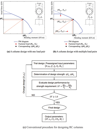
Design optimizations of round reinforced concrete columns based on artificial neural networks (ANNs) have been investigated in previous studies with only one pair of axial load ($P_u$) and bending moment ($M_u$). In this study, ANNs are generalized to be applicable to multiple load pairs by reshaping weight matrices of ANNs to prevent retraining of ANNs on the large datasets. Generalized ANN-based Lagrange optimizations are proposed for structural designs of round reinforced concrete columns with multiple load combinations. The present study modularizes the weight matrix of ANNs which considers one load pair to completely capture multiple factored loads. An optimal design by ANNs based on the modularized weight matrix and Lagrange optimization techniques using the Karush–Kuhn–Tucker (KKT) conditions was performed and validated with large datasets. Design examples performed by an ANN-based method and structural mechanics demonstrate accuracies of safety factors (SF) as small as 1% − 2%, which confirms the applicability of the proposed ANNs. Based on the present study, ANNs with modularized weight matrices aid engineers in optimizing round reinforced concrete columns subject to multiple loads.

KEYWORDS:

• Artificial neural networks
• modularized weight matrices
• reinforced concrete columns
• multiple load combinations
• Lagrange with Karush-Kuhn-Tucker conditions

1. Introduction

A breakthrough in applying machine learning (ML) techniques and optimization algorithms in the area of the civil engineering has been recently seen. ANN is an information-processing technique inspired by the human biological system, which aims to discover certain trends among input and output parameters of large datasets. Hong et al. (2021a) implemented ANN-based design charts for doubly reinforced concrete beams in reverse design problems. Other studies use ANN’s learning algorithm to allow ANNs to learn from material and structural behaviors. ANN-based models for structural analysis and design of RC columns were addressed by Kaarthikeyan(2016) and Charalampakis and Papanikolaou (2021) Although these studies developed rapid designs, they did not validate the developed ML models in practical design.

In the present study, conventional designs of round concrete columns subject to multiple loads are replaced by ANNs. Round reinforced concrete columns are usually designed to sustain axial forces ($P_u$) and bending moments ($M_u$). A pair of $P_u$, $M_u$ is regarded as one load pair or one load point on an interaction axial force–bending moment (P-M) diagram when designing columns. However, multiple load pairs must be sustained to practically design columns. This pivotal design aspect was rarely examined in previous studies. Lagaros and Papadrakakis (2015) tested six cases for optimization designs of RC columns while the investigated columns sustained one pair of $P_u$ and $M_u$ in each case. Hong and Cuong Nguyen, (2022a) performed design optimization of round concrete columns based on ANNs with only one pair of axial load ($P_u$) and bending moment ($M_u$). Hong et al. (2022b and Hong and Nguyen 2021) also studied a gradient-based approach utilizing Lagrange multiplier method (LMM) to optimize designs of RC uniaxial columns taking into account one load pair in strength limit state. Recently, Hong et al. (2022c) implemented ANNs and Lagrange optimization method to design RC round columns optimizing three objectives simultaneously and verified the method using a non-gradient Nondominated Sorting Genetic Algorithm – II. The suggested approach exhibited potential for structural designs. Specifically, uncommon structures such as tuned mass dampers were devised by Wang, L. et al. in their research [Wang et al. (2019a, 2019b, 2020a, 2020b, 2023a, 2022a, Wang et al. 2022b, 2023b; Wang, Zhou, and Shi 2023a, 2023b)].

The present study is divided into four main parts besides an introduction and research significance. Section 3 discusses a methodology of an ANN-based design of a round reinforced concrete column section to construct a generalized neural network considering multiple load pairs. Section 4 develops a hybrid optimization design method by implementing the Lagrange techniques based on an ANN. Section 5 validates the ANN-based optimization design, followed by a final section that concludes the study. In the present study, conventional design procedures of round concrete columns subject to multiple loads are replaced by ANN-based methods to optimize them. Safety factors (SF) were validated as small as 1% − 2% based on design examples performed by the ANN-based method and structural mechanics, which confirmed the accuracy of the proposed ANNs. The present study is developed on the basis of ANN-based structure designs shown in the books by Hong (2019, Hong 2023b, 2023c).

2. Research significance

Design optimizations of round reinforced concrete columns based on ANNs have been investigated in previous studies with only one pair of axial load ($P_u$) and bending moment ($M_u$), as shown in Figure 1 (a). In this study, ANNs are generalized to be applicable to any number of load pairs by reshaping an architecture of ANNs without needs of retraining the ANNs. A comprehensive objective function is also extracted from ANNs, which captures multiple load combinations, as illustrated in Figure 1(b), to allow an implementation of Lagrange Multiplier Method and Karush–Kuhn–Tucker (KKT) conditions ([Peel and Moon 2020)].

Figure 1. Conventional design of RC columns.

3. ANN-based design of round reinforced concrete column

3.1. Generation of large structural datasets

3.1.1. Forward design analysis and selection of design parameters

Figure 1(c) shows the conventional forward analysis to design an RC column. Design parameters include column dimensions ($\mathit{D}$), ${\rho }_s$, strain in the rebars (${\epsilon }_s$), and material properties, such as $f_c^{\prime }$ and $f_y$ to determine $\mathit{SF}$ which is a ratio of nominal section capacity to factored load $\left(\mathit{SF}=\mathit{\varphi }{P}_n/P_u=\mathit{\varphi }{M}_n/M_u\right)$. A design performance is evaluated in terms of strength requirements based on the condition of $\mathit{SF}\ge 1.0$, referring to section 10.5 – ACI 318–19. Economy and design sustainability are estimated based on $\mathit{C}{I}_c$,$\mathit{\hspace{0.17em}}{W}_c$, and $\mathit{C}{O}_2$ emissions, while design parameters are calculated accordingly. An interaction P-M diagram based on a nominal capacity of column sections ($M_n$, $P_n$) needs to be calculated when designing an RC column. A conventional design fits all load pairs inside a P-M diagram based on a trial-and-error process. $\mathit{SF}$s are selected as random variables instead of factored loads $P_u$ and $M_u$ when generating large datasets. Parameter (${\alpha }_{\mathit{e}/h}$) representing an eccentricity of applied axial loads is calculated when constructing P-M diagrams. However, ${\alpha }_{\mathit{e}/h}$ is not generated in large datasets, and not trained by the network either. Six inputs ($\mathit{D},\mathit{\hspace{0.17em}}{\rho }_s,f_c^{\prime },f_y,P_u,M_u$) are selected to represent the design requirements as shown in Table 1 whereas other parameters such as $\mathit{SF}$ and ${\epsilon }_s$, are calculated on an output-side. $\mathit{C}{I}_c$, $W_c$, and $\mathit{C}{O}_2$ emissions are also treated as output parameters.

Table 1. Design parameters’ nomenclature.

Notation	Nomenclature	Note
D	Column section diameter	Input parameters used in ANN to design RC columns
${\rho }_s$	Rebar ratio
$f_c^{\prime }$	Concrete strength
$f_y$	Rebar yield strength
$P_u$	Factored axial load
$M_u$	Factored bending moment
$\mathit{SF}$	Safety factor	Output parameters used in ANN to design RC columns
${\epsilon }_s$	Rebar strain
CIc	Cost index of column per height
CO2	CO2 emission per column height
Wc	Weight of column per column height
${\alpha }_{\mathit{e}/h}$	Angular eccentricity of applied load	Only applied to generate large dataset.

3.1.2. Generation of large structural datasets

Forward analysis of round RC columns was initially performed to select design input and output parameters when generating big datasets. A strain-compatibility-based structural analysis software of RC columns (called AutoCC) was written with MATLAB code. The software AutoCC is based on a conventional design following Building Code Requirements (Structural Concrete ACI 318–19 ([ACI Committee 2019])) shown in Figure 2). Big structural datasets are generated by AutoCC in which each input parameter will be randomly selected within its defined range shown in Table 2 whereas the corresponding outputs are calculated. Each data sample represents a set of randomly selected inputs and correspondingly calculated outputs. The generated datasets are divided into three subsets, such as training (70%), testing (15%), and validation datasets (15%). 70% of the generated datasets are used to train the ANN. The remaining datasets are divided equally into testing and validation datasets to test and validate the trained ANN.

Figure 2. ANN-based design of RC columns.

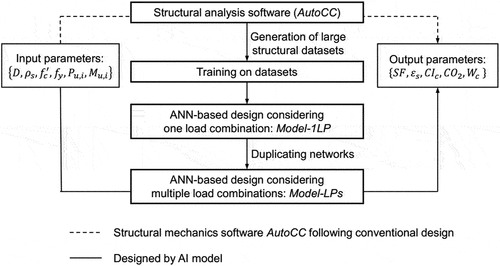
Table 2. Ranges to generate large dataset using structural mechanics-based software AutoCC.

Parameters	Random range to generate large datasets
D	400 mm ~1200 mm
	0.01 ~ 0.08
	20 MPa ~ 70 MPa
	300 MPa ~ 550 MPa
SF	0.1 ~ 3.0
	0 ~Π/2

One hundred thousand structural datasets are generated based on AutoCC. $\mathit{D},{\rho }_s,f_c^{\prime },f_y,\mathit{SF},{\alpha }_{\mathit{e}/h}$ are randomized input parameters within their ranges specified in Table 2. The corresponding output parameters $P_u,M_u,{\epsilon }_s,\mathit{C}{I}_c,\mathit{C}{O}_2,W_c$ are calculated on an output side of the AutoCC based on randomly selected inputs ($\mathit{D},{\rho }_s,f_c^{\prime },f_y,\mathit{SF},{\alpha }_{\mathit{e}/h}$). In particular, random ranges for $f_c^{\prime }$ and $f_y$ are 20–70 MPa and 300–550 MPa, respectively, for $\mathit{D}$ varying from 400 to 2000 mm. ${\rho }_s$ is restricted by minimum and maximum rebar ratios of 0.01 and 0.08 based on the design code ACI 318–19. The random values of $\mathit{SF}$ are controlled within 0.1–3.0, whereas those of ${\alpha }_{\mathit{e}/h}\mathit{\hspace{0.17em}}$which are not generated in large datasets are within the range of $0$–$\mathit{\pi }/2$. After generation, the large datasets are normalized in a range of − 1 to 1 before training, testing, and validating.

3.2. Formulation of networks with multiple load pairs by reusing weight matrices with one load pair

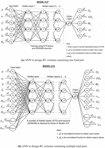
3.2.1. Topology of Model-1LP and Model-LPs

An ANN-based design of round RC columns with one load pair (Model-1LP) is performed based on design parameters including column diameter $\mathit{D}$, rebar ratio ${\rho }_s$, material properties (such as compressive strength of concrete ($f_c^{\prime }$), and yield strength of reinforcement ($f_y$)), and factored loads (axial load $P_u$ and bending moment $M_u$). These parameters are inputs of an ANN. The corresponding outputs include safety factor$\mathit{\hspace{0.17em}}\mathit{SF}$, strain of rebar ${\epsilon }_s$, cost index ($\mathit{C}{I}_c$), column weight ($W_c$), and $\mathit{C}{O}_2$ emission. A number of inputs and outputs used for ANNs with one load pair (Model-1LP) adjust and increase when multiple load pairs are considered for ANNs (Model-LPs) with multiple load pairs. An adjusted number of inputs and outputs, then, disturb the topology of Model-LPs. As a first step to fix the disturbance, Model-1LP with one load pair is trained, after which components of weight matrices, Model-1LP, corresponding to one load pair of are re-used to formulate weight matrices for a generalized ANN (Model-LPs) with multiple load pairs. The duplicated weight matrices of Model-LPs remove the needs of re-training Model-LPs to derive weight matrices with multiple loads. The duplicated weight matrices of Model-LPs help one derive objective functions, such as cost and $\mathit{C}{O}_2$ emissions which are used for optimizing Lagrange functions with LMM (refer to Section 4). The Lagrange function is well-behaved and well-defined to replace explicit mathematical functions because input parameters are mapped into output parameters through training. Figure 2 shows a design process implemented by ANN which is compared with the conventional design.

3.2.2. Network duplication

n multiple inputs load pairs $P_{\mathit{u},\mathit{i}}$, $M_{\mathit{u},\mathit{i}}$ result in n numbers of outputs $\mathit{S}{F}_i$ and ${\epsilon }_{\mathit{s},\mathit{i}}$, respectively. Output parameters in ANN are mapped by input parameters, such that mapped networks represent interconnected neural relationships between output and input parameters. Weight matrices with one load pair alter between the input layer and Hidden Layer 1 when input parameters increase when considering multiple load pairs for Model-LPs and hence, the components of weight matrices of Model-1LP corresponding to one load pair are reused to formulate weight matrices for a generalized ANN (Model-LPs) with multiple load pairs. Components of weight matrices of ANN (Model-1LP) corresponding to one load pair during mapping between input layer and Hidden Layer 1 can be duplicated and modularized to formulate a generalized ANN (Model-LPs) with multiple load pairs. However, after Hidden Layer 1, the topology of an ANN (Model-LPs) with multiple load pairs is unaltered because the hidden layers and neurons after Hidden Layer 1 are identical to those of ANN (Model-1LP), and hence, mapped networks for Model-LPs with multiple load pairs which links output parameters $\mathit{S}{F}_1,\mathit{S}{F}_2,\mathit{\hspace{0.17em}}\dots ,\mathit{\hspace{0.17em}}\mathit{S}{F}_n$ to input parameters can be treated similarly to the link of one SF to input parameters of ANN (Model-1LP) with one load pair after Hidden Layer 1.

Figure 3a shows the topology of Model-1LP for designing round RC columns subject to one load pair. However, the practical designs of round RC columns must simultaneously capture multiple load pairs. In generalized Model-LPs for n load pairs ($P_{\mathit{u},\mathit{i}},\mathit{\hspace{0.17em}}{M}_{\mathit{u},\mathit{i}}$, i = 1, … , n) shown in Figures 3b, 2n +4 input variables are considered in the input layers rather than six input parameters ($\mathit{D},{\rho }_s,f_c^{\prime },f_y,\mathit{SF},{\alpha }_{\mathit{e}/h}$) adapted for Model-1LP shown in Figure 3a. Input parameters 2n + 4 represent 2 × n load pairs ($P_{\mathit{u},\mathit{i}},\mathit{\hspace{0.17em}}{M}_{\mathit{u},\mathit{i}}$) + four input parameters ($\mathit{D},{\rho }_s,f_c^{\prime },f_y$) which are unaffected by duplications. Output parameters corresponding to n load pairs ($P_{\mathit{u},\mathit{i}},\mathit{\hspace{0.17em}}{M}_{\mathit{u},\mathit{i}}$, i = 1, … , n) are also adjusted by adding $\mathit{S}{F}_i$ and ${\epsilon }_{\mathit{s},\mathit{i}}$ on an output-side as shown in Figure 3b. The altered input parameters (2n + 4) directly affect the mapping input parameters to Hidden Layer 1, altering only weight matrices in the first hidden layer ${\omega }_{in\mathrm{put}}^{\left(1\right)}$. However, the rest of the hidden layers of Model-LPs do not alter, remaining the same as those of Model-1LP.

Figure 3. Topology of ANN to design RC columns.

Equation 1(1) $\underset{\mathit{\hspace{0.17em}}}{\underbrace{y_4\left(\mathit{SF}\right)}}\left[1\times 1\right]=g_{SF}^D\left(f_{\mathit{linear}}\left(\underset{\left[1\times 20\right]}{\underbrace{{\omega }_{SF}^{\left(out\right)}}}{f}_{\mathit{tanh}}\left(\underset{\left[20\times 20\right]}{\underbrace{{\omega }_{SF}^k}}\dots f_{\mathit{tanh}}\left(\underset{\left[20\times 6\right]}{\underbrace{{\omega }_{SF}^{\left(1\right)}}}\mathit{\hspace{0.17em}}\underset{\left[6\times 1\right]}{\underbrace{g^N\left(\mathit{x}\right)}}+\underset{\left[20\times 1\right]}{\underbrace{b_{SF}^{\left(1\right)}}}\right)\dots +\underset{\left[20\times 1\right]}{\underbrace{b_{SF}^{\left(k\right)}}}\right)+\mathit{\hspace{0.17em}}\underset{\left[1\times 1\right]}{\underbrace{b_{SF}^{\left(out\right)}}}\mathit{\hspace{0.17em}}\right)\mathit{\hspace{0.17em}}\right)$(1) represents an ANN for an output parameter $\mathit{SF}$ with one load pair Villarrubia et al. (2018) in which the input vector $\mathbf{x}$ contains normalized values of $\left\{\mathit{D},{\rho }_s,\mathit{\hspace{0.17em}}{f}_c^{\prime },\mathit{\hspace{0.17em}}{f}_y,\mathit{\hspace{0.17em}}{P}_u,M_u\right\}$. Neural values of the first hidden layer (Hidden Layer 1) are calculated based on the input parameters $\mathbf{x}$ using the first weight matrix ${\omega }_{SF}^{\left(1\right)}$ and bias matrix$\mathit{\hspace{0.17em}}{b}_{SF}^{\left(1\right)}$. Neural values in Hidden Layer 1 are activated by the tansig activation function ($f_{\mathit{tansig}})$. Neural values of the successive hidden layers are calculated using weight matrix ${\omega }_{SF}^{\left(k\right)}$ and bias matrix $b_{SF}^{\left(k\right)}$, where k represents a k^th hidden layer under consideration. Note that the best training of the output parameter $\mathit{SF}$ is based on 10 layers and 20 neurons as shown in Table 3. Only one neuron value is calculated at the output layer which is activated by the linear activation function ($f_{\mathit{linear}}$) before being de-normalized to obtain output ${\mathit{y}}_4$ of the original scale as $\mathit{SF}$.

Table 3. Training results and accuracies from using tansig activation function.

6 Inputs ($\mathit{D},{\rho }_s,f_c^{\prime },f_y,P_u,M_u$) − 5 Outputs ($\mathit{SF},{\epsilon }_s,\mathit{C}{I}_c,\mathit{C}{O}_2,W_c$)
PTM − 100,000 data − 100,000 suggested epochs – tansig activation function
Output	Layers	Neurons	Best Epoch	Stopped Epoch	Test MSE	R at Best Epoch
$\mathit{SF}$	10	20	98,390	99,390	4.0.E–04	0.9994
${\epsilon }_s$	10	80	66,717	66,817	2.0.E–05	0.9998
$\mathit{C}{I}_c$	10	20	13,224	14,224	7.6.E–07	1.0000
$\mathit{C}{O}_2$	5	20	43,211	44,211	6.8.E–08	1.0000
$W_c$	5	80	40,073	41,073	5.9.E–07	1.0000

Equation 2(2) $\begin{array}{rl}& \underset{\left[1\times 1\right]}{\underbrace{y\left(S{F}_i\right)}}=g_{S{F}_i}^{\mathit{D}}\left.\left(f_{\mathit{linear}}\left(\underset{\left[1\times 20\right]}{\underbrace{{\mathit{\omega }}_{S{F}_i}^{\left(\mathit{out}\right)}}}{f}_{\mathit{tanh}}\right.\right.\left.\left(\underset{\left[20\times 20\right]}{\underbrace{{\mathit{\omega }}_{S{F}_i}^{\mathit{k}}}}\dots f_{\mathit{tanh}}\left(\underset{\left[20\times \left(2\mathit{n}+4\right)\right]}{\underbrace{{\mathit{\omega }}_{S{F}_i}^{\left(1\right)}}}\underset{\left[\left(2\mathit{n}+4\right)\times 1\right]}{\underbrace{g^N\left(\mathit{x}\right)}}\text{break}+\underset{\left[20\times 1\right]}{\underbrace{{\mathit{b}}_{S{F}_i}^{\left(1\right)}}}\right)\dots +\underset{\left[20\times 1\right]}{\underbrace{{\mathit{b}}_{S{F}_i}^{\left(\mathit{k}\right)}}}\right)+\underset{\left[1\times 1\right]}{\underbrace{{\mathit{b}}_{S{F}_i}^{\left(\mathit{out}\right)}}}\right)\right)\\ & \mathit{i}\mathit{\hspace{0.17em}}=\mathit{\hspace{0.17em}}1,\mathit{\hspace{0.17em}}2,\mathit{\hspace{0.17em}}\dots ,\mathit{\hspace{0.17em}}\mathit{n}\left(\mathit{n}\mathit{\hspace{0.17em}}=\mathit{\hspace{0.17em}}\mathit{number}\mathit{\hspace{0.17em}}\mathit{of}\mathit{\hspace{0.17em}}\mathit{load}\mathit{\hspace{0.17em}}\mathit{pairs}\right)\end{array}$(2) describes an ANN for output parameters $\mathit{S}{F}_i$ with i = n load pairs Villarrubia et al. (2018). Weight matrix Model-LPs is obtained from Model-1LP. The increased input parameters $\mathbf{x}$ contain (2n +4) normalized variables, which increase the size of the weight matrix of the first hidden layer ${\mathit{\omega }}_{S{F}_i}^{\left(1\right)}$ to a $20\times \left(2\mathit{n}+4\right)$ matrix shown in Equation 2(2) $\begin{array}{rl}& \underset{\left[1\times 1\right]}{\underbrace{y\left(S{F}_i\right)}}=g_{S{F}_i}^{\mathit{D}}\left.\left(f_{\mathit{linear}}\left(\underset{\left[1\times 20\right]}{\underbrace{{\mathit{\omega }}_{S{F}_i}^{\left(\mathit{out}\right)}}}{f}_{\mathit{tanh}}\right.\right.\left.\left(\underset{\left[20\times 20\right]}{\underbrace{{\mathit{\omega }}_{S{F}_i}^{\mathit{k}}}}\dots f_{\mathit{tanh}}\left(\underset{\left[20\times \left(2\mathit{n}+4\right)\right]}{\underbrace{{\mathit{\omega }}_{S{F}_i}^{\left(1\right)}}}\underset{\left[\left(2\mathit{n}+4\right)\times 1\right]}{\underbrace{g^N\left(\mathit{x}\right)}}\text{break}+\underset{\left[20\times 1\right]}{\underbrace{{\mathit{b}}_{S{F}_i}^{\left(1\right)}}}\right)\dots +\underset{\left[20\times 1\right]}{\underbrace{{\mathit{b}}_{S{F}_i}^{\left(\mathit{k}\right)}}}\right)+\underset{\left[1\times 1\right]}{\underbrace{{\mathit{b}}_{S{F}_i}^{\left(\mathit{out}\right)}}}\right)\right)\\ & \mathit{i}\mathit{\hspace{0.17em}}=\mathit{\hspace{0.17em}}1,\mathit{\hspace{0.17em}}2,\mathit{\hspace{0.17em}}\dots ,\mathit{\hspace{0.17em}}\mathit{n}\left(\mathit{n}\mathit{\hspace{0.17em}}=\mathit{\hspace{0.17em}}\mathit{number}\mathit{\hspace{0.17em}}\mathit{of}\mathit{\hspace{0.17em}}\mathit{load}\mathit{\hspace{0.17em}}\mathit{pairs}\right)\end{array}$(2) from a $20\times 6$ matrix of ${\omega }_{SF}^{\left(1\right)}$ shown in Equation 1(1) $\underset{\mathit{\hspace{0.17em}}}{\underbrace{y_4\left(\mathit{SF}\right)}}\left[1\times 1\right]=g_{SF}^D\left(f_{\mathit{linear}}\left(\underset{\left[1\times 20\right]}{\underbrace{{\omega }_{SF}^{\left(out\right)}}}{f}_{\mathit{tanh}}\left(\underset{\left[20\times 20\right]}{\underbrace{{\omega }_{SF}^k}}\dots f_{\mathit{tanh}}\left(\underset{\left[20\times 6\right]}{\underbrace{{\omega }_{SF}^{\left(1\right)}}}\mathit{\hspace{0.17em}}\underset{\left[6\times 1\right]}{\underbrace{g^N\left(\mathit{x}\right)}}+\underset{\left[20\times 1\right]}{\underbrace{b_{SF}^{\left(1\right)}}}\right)\dots +\underset{\left[20\times 1\right]}{\underbrace{b_{SF}^{\left(k\right)}}}\right)+\mathit{\hspace{0.17em}}\underset{\left[1\times 1\right]}{\underbrace{b_{SF}^{\left(out\right)}}}\mathit{\hspace{0.17em}}\right)\mathit{\hspace{0.17em}}\right)$(1) . The other components of the weight and bias matrices of the hidden and output layers are unchanged, which is shown in Equation 2(2) $\begin{array}{rl}& \underset{\left[1\times 1\right]}{\underbrace{y\left(S{F}_i\right)}}=g_{S{F}_i}^{\mathit{D}}\left.\left(f_{\mathit{linear}}\left(\underset{\left[1\times 20\right]}{\underbrace{{\mathit{\omega }}_{S{F}_i}^{\left(\mathit{out}\right)}}}{f}_{\mathit{tanh}}\right.\right.\left.\left(\underset{\left[20\times 20\right]}{\underbrace{{\mathit{\omega }}_{S{F}_i}^{\mathit{k}}}}\dots f_{\mathit{tanh}}\left(\underset{\left[20\times \left(2\mathit{n}+4\right)\right]}{\underbrace{{\mathit{\omega }}_{S{F}_i}^{\left(1\right)}}}\underset{\left[\left(2\mathit{n}+4\right)\times 1\right]}{\underbrace{g^N\left(\mathit{x}\right)}}\text{break}+\underset{\left[20\times 1\right]}{\underbrace{{\mathit{b}}_{S{F}_i}^{\left(1\right)}}}\right)\dots +\underset{\left[20\times 1\right]}{\underbrace{{\mathit{b}}_{S{F}_i}^{\left(\mathit{k}\right)}}}\right)+\underset{\left[1\times 1\right]}{\underbrace{{\mathit{b}}_{S{F}_i}^{\left(\mathit{out}\right)}}}\right)\right)\\ & \mathit{i}\mathit{\hspace{0.17em}}=\mathit{\hspace{0.17em}}1,\mathit{\hspace{0.17em}}2,\mathit{\hspace{0.17em}}\dots ,\mathit{\hspace{0.17em}}\mathit{n}\left(\mathit{n}\mathit{\hspace{0.17em}}=\mathit{\hspace{0.17em}}\mathit{number}\mathit{\hspace{0.17em}}\mathit{of}\mathit{\hspace{0.17em}}\mathit{load}\mathit{\hspace{0.17em}}\mathit{pairs}\right)\end{array}$(2) and the topology of network Model-LPs shown in Figure 3. The output parameter $\mathit{SF}$ shown in Equation 1(1) $\underset{\mathit{\hspace{0.17em}}}{\underbrace{y_4\left(\mathit{SF}\right)}}\left[1\times 1\right]=g_{SF}^D\left(f_{\mathit{linear}}\left(\underset{\left[1\times 20\right]}{\underbrace{{\omega }_{SF}^{\left(out\right)}}}{f}_{\mathit{tanh}}\left(\underset{\left[20\times 20\right]}{\underbrace{{\omega }_{SF}^k}}\dots f_{\mathit{tanh}}\left(\underset{\left[20\times 6\right]}{\underbrace{{\omega }_{SF}^{\left(1\right)}}}\mathit{\hspace{0.17em}}\underset{\left[6\times 1\right]}{\underbrace{g^N\left(\mathit{x}\right)}}+\underset{\left[20\times 1\right]}{\underbrace{b_{SF}^{\left(1\right)}}}\right)\dots +\underset{\left[20\times 1\right]}{\underbrace{b_{SF}^{\left(k\right)}}}\right)+\mathit{\hspace{0.17em}}\underset{\left[1\times 1\right]}{\underbrace{b_{SF}^{\left(out\right)}}}\mathit{\hspace{0.17em}}\right)\mathit{\hspace{0.17em}}\right)$(1) calculated by network Model-1LP is equivalent to $\mathit{S}{F}_i$ shown in Equation 2 calculated by Model-LPs which is governed by the i-th load pair ($P_{\mathit{u},\mathit{i}},\mathit{\hspace{0.17em}}{M}_{\mathit{u},\mathit{i}}$) .

(1) $\underset{\mathit{\hspace{0.17em}}}{\underbrace{y_4\left(\mathit{SF}\right)}}\left[1\times 1\right]=g_{SF}^D\left(f_{\mathit{linear}}\left(\underset{\left[1\times 20\right]}{\underbrace{{\omega }_{SF}^{\left(out\right)}}}{f}_{\mathit{tanh}}\left(\underset{\left[20\times 20\right]}{\underbrace{{\omega }_{SF}^k}}\dots f_{\mathit{tanh}}\left(\underset{\left[20\times 6\right]}{\underbrace{{\omega }_{SF}^{\left(1\right)}}}\mathit{\hspace{0.17em}}\underset{\left[6\times 1\right]}{\underbrace{g^N\left(\mathit{x}\right)}}+\underset{\left[20\times 1\right]}{\underbrace{b_{SF}^{\left(1\right)}}}\right)\dots +\underset{\left[20\times 1\right]}{\underbrace{b_{SF}^{\left(k\right)}}}\right)+\mathit{\hspace{0.17em}}\underset{\left[1\times 1\right]}{\underbrace{b_{SF}^{\left(out\right)}}}\mathit{\hspace{0.17em}}\right)\mathit{\hspace{0.17em}}\right)$(1)

(2) $\begin{array}{rl}& \underset{\left[1\times 1\right]}{\underbrace{y\left(S{F}_i\right)}}=g_{S{F}_i}^{\mathit{D}}\left.\left(f_{\mathit{linear}}\left(\underset{\left[1\times 20\right]}{\underbrace{{\mathit{\omega }}_{S{F}_i}^{\left(\mathit{out}\right)}}}{f}_{\mathit{tanh}}\right.\right.\left.\left(\underset{\left[20\times 20\right]}{\underbrace{{\mathit{\omega }}_{S{F}_i}^{\mathit{k}}}}\dots f_{\mathit{tanh}}\left(\underset{\left[20\times \left(2\mathit{n}+4\right)\right]}{\underbrace{{\mathit{\omega }}_{S{F}_i}^{\left(1\right)}}}\underset{\left[\left(2\mathit{n}+4\right)\times 1\right]}{\underbrace{g^N\left(\mathit{x}\right)}}\text{break}+\underset{\left[20\times 1\right]}{\underbrace{{\mathit{b}}_{S{F}_i}^{\left(1\right)}}}\right)\dots +\underset{\left[20\times 1\right]}{\underbrace{{\mathit{b}}_{S{F}_i}^{\left(\mathit{k}\right)}}}\right)+\underset{\left[1\times 1\right]}{\underbrace{{\mathit{b}}_{S{F}_i}^{\left(\mathit{out}\right)}}}\right)\right)\\ & \mathit{i}\mathit{\hspace{0.17em}}=\mathit{\hspace{0.17em}}1,\mathit{\hspace{0.17em}}2,\mathit{\hspace{0.17em}}\dots ,\mathit{\hspace{0.17em}}\mathit{n}\left(\mathit{n}\mathit{\hspace{0.17em}}=\mathit{\hspace{0.17em}}\mathit{number}\mathit{\hspace{0.17em}}\mathit{of}\mathit{\hspace{0.17em}}\mathit{load}\mathit{\hspace{0.17em}}\mathit{pairs}\right)\end{array}$(2)

3.2.3. Formulation of weight matrices with multiple load pairs

An output parameter $\mathit{S}{F}_i$ in Model-LPs should have a mapping trait similar to that of an output $\mathit{SF}$ in Model-1LP because their components related to the applied load pairs of weight matrices (${\mathit{\omega }}_{S{F}_i}^{\left(1\right)})$for Hidden Layer 1 of in Model-LPs is duplicated from ${\omega }_{SF}^{\left(1\right)}$ of Model-1LP shown in Equation 3(3) $\begin{array}{rl}& {\left[\begin{array}{c}Ne\mathrm{uron}1\\ Ne\mathrm{uron}2\\ ⋮\\ Ne\mathrm{uron}20\end{array}\right]}_{20\times 1}^{(1),SF}\\ & =\mathit{f}tan\mathit{sig}\left({\left[\begin{array}{cccccc}1\mathit{st}& 2\mathit{nd}& 3\mathit{rd}& 4\mathit{th}& 5\mathit{th}& 6\mathit{th}\\ {\mathit{\omega }}_{1,1}& {\omega }_{1,2}& {\omega }_{1,3}& {\omega }_{1,4}& {\omega }_{1,5}& {\omega }_{1,6}\\ {\omega }_{2,1}& {\omega }_{2,2}& {\omega }_{2,3}& {\omega }_{2,4}& {\omega }_{2,5}& {\omega }_{2,6}\\ ⋮& ⋮& ⋮& ⋮& ⋮& ⋮\\ {\omega }_{20,1}& {\omega }_{20,2}& {\omega }_{20,3}& {\omega }_{20,4}& {\omega }_{20,5}& {\omega }_{20,6}\end{array}\right]}_{20\mathit{x}6}^{(1),\mathit{SF}}\text{break}{\left[\begin{array}{cc}\mathit{D}& 1\mathit{st}\\ {\rho }_S& 2\mathit{nd}\\ f_c& 3\mathit{rd}\\ f_y& 4\mathit{th}\\ P_u& 5\mathit{th}\\ M_u& 6\mathit{th}\end{array}\right]}_{6\times 1}+{\left[\begin{array}{c}{b}_1\\ b_2\\ ⋮\\ b_{20}\end{array}\right]}_{20\times 1}^{(1),\mathit{SF}}\right)\end{array}$(3) (Hong 2023a).

Let’s derive the weight matrix at the first hidden layer of the ANN Model-LPs subject to multiple load pairs. Firstly, the weight matrix of $\mathit{S}{F}_1\left(\mathit{i}=1\right)$at the first hidden layer of the ANN Model-LPs is derived when Load Pair 1 ($P_{\mathit{u},1},\mathit{\hspace{0.17em}}{M}_{\mathit{u},1}$) is applied. The weight matrix of Hidden Layer 1 for $\mathit{S}{F}_1$ of Model-LPs ${\mathit{\omega }}_{S{F}_1}^{\left(1\right)}$ shown in Equation 4(4) $\begin{array}{rl}& {\left[\begin{array}{c}\mathit{Neuron}1\\ \mathit{Neuron}2\\ ⋮\\ \mathit{Neuron}20\end{array}\right]}_{20\times (2\mathit{n}+4)}^{(1),S{F}_1}=f_{\mathit{tansig}}\left(\begin{array}{ccc}\underset{[20\times (2\mathit{n}+4)]\mathit{\hspace{0.17em}}}{\underbrace{{\mathit{\omega }}_{S{F}_1}^{(1)}}}& \underset{[(2\mathit{n}+4)\times 1]}{\underbrace{{\mathbf{x}}^{\mathrm{in}}}}& \underset{[20\times 1]}{\underbrace{{\mathbf{b}}_{S{F}_1}^{(1)}}}\end{array}\right)\\ & =f_{\mathit{tanh}}{\left[\begin{array}{ccccccccccc}1\mathit{st}& 2\mathit{nd}& 3\mathit{rd}& 4\mathit{th}& 5\mathit{th}& 6\mathit{th}& 7\mathit{th}& 8\mathit{th}& \dots & (2\mathit{n}+3)\mathit{th}& (2\mathit{n}+4)\mathit{th}\\ {\mathit{\omega }}_{1,1}& {\omega }_{1,2}& {\omega }_{1,3}& {\omega }_{1,4}& {\omega }_{1,5}& {\omega }_{1,6}& 0& 0& \cdots & 0& 0\\ {\omega }_{2,1}& {\omega }_{2,2}& {\omega }_{2,3}& {\omega }_{2,4}& {\omega }_{2,5}& {\omega }_{2,6}& 0& 0& \cdots & 0& 0\\ ⋮& ⋮& ⋮& ⋮& ⋮& ⋮& ⋮& ⋮& \ddots & ⋮& ⋮\\ {\omega }_{20,1}& {\omega }_{20,2}& {\omega }_{20,3}& {\omega }_{20,4}& {\omega }_{20,5}& {\omega }_{20,6}& 0& 0& \cdots & 0& 0\end{array}\right]}_{20\times (2\mathit{n}+4)}^{(1),\mathit{S}{F}_1}\text{break}\times {\left[\begin{array}{cc}\mathit{D}& 1\mathit{st}\\ {\rho }_S& 2\mathit{nd}\\ {f^{\prime }}_{\mathit{C}}& 3\mathit{rd}\\ f_y& 4\mathit{th}\\ P_{\mathit{u},1}& 5\mathit{th}\\ M_{\mathit{u},2}& 6\mathit{th}\\ P_{\mathit{u},2}& 7\mathit{th}\\ M_{\mathit{u},2}& 8\mathit{th}\\ ⋮& ⋮\\ P_{\mathit{u},\mathit{n}}& (2\mathit{n}+3)\mathit{th}\\ M_{\mathit{u},\mathit{n}}& (2\mathit{n}+4)\mathit{th}\end{array}\right]}_{(2\mathit{n}+4)\times 1}+{\left[\begin{array}{c}{b}_1\\ b_2\\ ⋮\\ b_{20}\end{array}\right]}_{20\times 1}^{(1),\mathit{S}{F}_1}\end{array}$(4) (Hong 2023a) is modified from the weight matrix of Model-1LP shown in Equation 3(3) $\begin{array}{rl}& {\left[\begin{array}{c}Ne\mathrm{uron}1\\ Ne\mathrm{uron}2\\ ⋮\\ Ne\mathrm{uron}20\end{array}\right]}_{20\times 1}^{(1),SF}\\ & =\mathit{f}tan\mathit{sig}\left({\left[\begin{array}{cccccc}1\mathit{st}& 2\mathit{nd}& 3\mathit{rd}& 4\mathit{th}& 5\mathit{th}& 6\mathit{th}\\ {\mathit{\omega }}_{1,1}& {\omega }_{1,2}& {\omega }_{1,3}& {\omega }_{1,4}& {\omega }_{1,5}& {\omega }_{1,6}\\ {\omega }_{2,1}& {\omega }_{2,2}& {\omega }_{2,3}& {\omega }_{2,4}& {\omega }_{2,5}& {\omega }_{2,6}\\ ⋮& ⋮& ⋮& ⋮& ⋮& ⋮\\ {\omega }_{20,1}& {\omega }_{20,2}& {\omega }_{20,3}& {\omega }_{20,4}& {\omega }_{20,5}& {\omega }_{20,6}\end{array}\right]}_{20\mathit{x}6}^{(1),\mathit{SF}}\text{break}{\left[\begin{array}{cc}\mathit{D}& 1\mathit{st}\\ {\rho }_S& 2\mathit{nd}\\ f_c& 3\mathit{rd}\\ f_y& 4\mathit{th}\\ P_u& 5\mathit{th}\\ M_u& 6\mathit{th}\end{array}\right]}_{6\times 1}+{\left[\begin{array}{c}{b}_1\\ b_2\\ ⋮\\ b_{20}\end{array}\right]}_{20\times 1}^{(1),\mathit{SF}}\right)\end{array}$(3) .

Equations 3(3) $\begin{array}{rl}& {\left[\begin{array}{c}Ne\mathrm{uron}1\\ Ne\mathrm{uron}2\\ ⋮\\ Ne\mathrm{uron}20\end{array}\right]}_{20\times 1}^{(1),SF}\\ & =\mathit{f}tan\mathit{sig}\left({\left[\begin{array}{cccccc}1\mathit{st}& 2\mathit{nd}& 3\mathit{rd}& 4\mathit{th}& 5\mathit{th}& 6\mathit{th}\\ {\mathit{\omega }}_{1,1}& {\omega }_{1,2}& {\omega }_{1,3}& {\omega }_{1,4}& {\omega }_{1,5}& {\omega }_{1,6}\\ {\omega }_{2,1}& {\omega }_{2,2}& {\omega }_{2,3}& {\omega }_{2,4}& {\omega }_{2,5}& {\omega }_{2,6}\\ ⋮& ⋮& ⋮& ⋮& ⋮& ⋮\\ {\omega }_{20,1}& {\omega }_{20,2}& {\omega }_{20,3}& {\omega }_{20,4}& {\omega }_{20,5}& {\omega }_{20,6}\end{array}\right]}_{20\mathit{x}6}^{(1),\mathit{SF}}\text{break}{\left[\begin{array}{cc}\mathit{D}& 1\mathit{st}\\ {\rho }_S& 2\mathit{nd}\\ f_c& 3\mathit{rd}\\ f_y& 4\mathit{th}\\ P_u& 5\mathit{th}\\ M_u& 6\mathit{th}\end{array}\right]}_{6\times 1}+{\left[\begin{array}{c}{b}_1\\ b_2\\ ⋮\\ b_{20}\end{array}\right]}_{20\times 1}^{(1),\mathit{SF}}\right)\end{array}$(3) and 4(4) $\begin{array}{rl}& {\left[\begin{array}{c}\mathit{Neuron}1\\ \mathit{Neuron}2\\ ⋮\\ \mathit{Neuron}20\end{array}\right]}_{20\times (2\mathit{n}+4)}^{(1),S{F}_1}=f_{\mathit{tansig}}\left(\begin{array}{ccc}\underset{[20\times (2\mathit{n}+4)]\mathit{\hspace{0.17em}}}{\underbrace{{\mathit{\omega }}_{S{F}_1}^{(1)}}}& \underset{[(2\mathit{n}+4)\times 1]}{\underbrace{{\mathbf{x}}^{\mathrm{in}}}}& \underset{[20\times 1]}{\underbrace{{\mathbf{b}}_{S{F}_1}^{(1)}}}\end{array}\right)\\ & =f_{\mathit{tanh}}{\left[\begin{array}{ccccccccccc}1\mathit{st}& 2\mathit{nd}& 3\mathit{rd}& 4\mathit{th}& 5\mathit{th}& 6\mathit{th}& 7\mathit{th}& 8\mathit{th}& \dots & (2\mathit{n}+3)\mathit{th}& (2\mathit{n}+4)\mathit{th}\\ {\mathit{\omega }}_{1,1}& {\omega }_{1,2}& {\omega }_{1,3}& {\omega }_{1,4}& {\omega }_{1,5}& {\omega }_{1,6}& 0& 0& \cdots & 0& 0\\ {\omega }_{2,1}& {\omega }_{2,2}& {\omega }_{2,3}& {\omega }_{2,4}& {\omega }_{2,5}& {\omega }_{2,6}& 0& 0& \cdots & 0& 0\\ ⋮& ⋮& ⋮& ⋮& ⋮& ⋮& ⋮& ⋮& \ddots & ⋮& ⋮\\ {\omega }_{20,1}& {\omega }_{20,2}& {\omega }_{20,3}& {\omega }_{20,4}& {\omega }_{20,5}& {\omega }_{20,6}& 0& 0& \cdots & 0& 0\end{array}\right]}_{20\times (2\mathit{n}+4)}^{(1),\mathit{S}{F}_1}\text{break}\times {\left[\begin{array}{cc}\mathit{D}& 1\mathit{st}\\ {\rho }_S& 2\mathit{nd}\\ {f^{\prime }}_{\mathit{C}}& 3\mathit{rd}\\ f_y& 4\mathit{th}\\ P_{\mathit{u},1}& 5\mathit{th}\\ M_{\mathit{u},2}& 6\mathit{th}\\ P_{\mathit{u},2}& 7\mathit{th}\\ M_{\mathit{u},2}& 8\mathit{th}\\ ⋮& ⋮\\ P_{\mathit{u},\mathit{n}}& (2\mathit{n}+3)\mathit{th}\\ M_{\mathit{u},\mathit{n}}& (2\mathit{n}+4)\mathit{th}\end{array}\right]}_{(2\mathit{n}+4)\times 1}+{\left[\begin{array}{c}{b}_1\\ b_2\\ ⋮\\ b_{20}\end{array}\right]}_{20\times 1}^{(1),\mathit{S}{F}_1}\end{array}$(4) show that the components of the weight matrices related to the first four input parameters $\mathit{D},{\rho }_s,\mathit{\hspace{0.17em}}{f}_c^{\prime },\mathit{\hspace{0.17em}}{f}_y$ are unaffected when formulating weight matrices of Model-LPs. Note that $\mathit{S}{F}_i$ is determined as a ratio of the nominal strength to factored load ($\mathit{S}{F}_i=\mathit{\varphi }{P}_{\mathit{n},\mathit{i}}/P_{\mathit{u},\mathit{i}}=\mathit{\varphi }{M}_{\mathit{n},\mathit{i}}/M_{\mathit{u},\mathit{i}}$), indicating that each value of $\mathit{S}{F}_i$ is governed by its corresponding load pair ($P_{\mathit{u},\mathit{i}},\mathit{\hspace{0.17em}}{M}_{\mathit{u},\mathit{i}}$). The components of ${\mathit{\omega }}_{S{F}_1}^{\left(1\right)}$ matrix corresponding to factored loads $P_{\mathit{u},1}$ and $M_{\mathit{u},1}$ shown in Equation 4(4) $\begin{array}{rl}& {\left[\begin{array}{c}\mathit{Neuron}1\\ \mathit{Neuron}2\\ ⋮\\ \mathit{Neuron}20\end{array}\right]}_{20\times (2\mathit{n}+4)}^{(1),S{F}_1}=f_{\mathit{tansig}}\left(\begin{array}{ccc}\underset{[20\times (2\mathit{n}+4)]\mathit{\hspace{0.17em}}}{\underbrace{{\mathit{\omega }}_{S{F}_1}^{(1)}}}& \underset{[(2\mathit{n}+4)\times 1]}{\underbrace{{\mathbf{x}}^{\mathrm{in}}}}& \underset{[20\times 1]}{\underbrace{{\mathbf{b}}_{S{F}_1}^{(1)}}}\end{array}\right)\\ & =f_{\mathit{tanh}}{\left[\begin{array}{ccccccccccc}1\mathit{st}& 2\mathit{nd}& 3\mathit{rd}& 4\mathit{th}& 5\mathit{th}& 6\mathit{th}& 7\mathit{th}& 8\mathit{th}& \dots & (2\mathit{n}+3)\mathit{th}& (2\mathit{n}+4)\mathit{th}\\ {\mathit{\omega }}_{1,1}& {\omega }_{1,2}& {\omega }_{1,3}& {\omega }_{1,4}& {\omega }_{1,5}& {\omega }_{1,6}& 0& 0& \cdots & 0& 0\\ {\omega }_{2,1}& {\omega }_{2,2}& {\omega }_{2,3}& {\omega }_{2,4}& {\omega }_{2,5}& {\omega }_{2,6}& 0& 0& \cdots & 0& 0\\ ⋮& ⋮& ⋮& ⋮& ⋮& ⋮& ⋮& ⋮& \ddots & ⋮& ⋮\\ {\omega }_{20,1}& {\omega }_{20,2}& {\omega }_{20,3}& {\omega }_{20,4}& {\omega }_{20,5}& {\omega }_{20,6}& 0& 0& \cdots & 0& 0\end{array}\right]}_{20\times (2\mathit{n}+4)}^{(1),\mathit{S}{F}_1}\text{break}\times {\left[\begin{array}{cc}\mathit{D}& 1\mathit{st}\\ {\rho }_S& 2\mathit{nd}\\ {f^{\prime }}_{\mathit{C}}& 3\mathit{rd}\\ f_y& 4\mathit{th}\\ P_{\mathit{u},1}& 5\mathit{th}\\ M_{\mathit{u},2}& 6\mathit{th}\\ P_{\mathit{u},2}& 7\mathit{th}\\ M_{\mathit{u},2}& 8\mathit{th}\\ ⋮& ⋮\\ P_{\mathit{u},\mathit{n}}& (2\mathit{n}+3)\mathit{th}\\ M_{\mathit{u},\mathit{n}}& (2\mathit{n}+4)\mathit{th}\end{array}\right]}_{(2\mathit{n}+4)\times 1}+{\left[\begin{array}{c}{b}_1\\ b_2\\ ⋮\\ b_{20}\end{array}\right]}_{20\times 1}^{(1),\mathit{S}{F}_1}\end{array}$(4) are ${\mathit{\omega }}_{1,5},\mathit{\hspace{0.17em}}{\mathit{\omega }}_{1,6}$ which are the same weight components with respect to $P_u$ and $\mathit{\hspace{0.17em}}{M}_u$ in Model-1LP shown in Equation 3(3) $\begin{array}{rl}& {\left[\begin{array}{c}Ne\mathrm{uron}1\\ Ne\mathrm{uron}2\\ ⋮\\ Ne\mathrm{uron}20\end{array}\right]}_{20\times 1}^{(1),SF}\\ & =\mathit{f}tan\mathit{sig}\left({\left[\begin{array}{cccccc}1\mathit{st}& 2\mathit{nd}& 3\mathit{rd}& 4\mathit{th}& 5\mathit{th}& 6\mathit{th}\\ {\mathit{\omega }}_{1,1}& {\omega }_{1,2}& {\omega }_{1,3}& {\omega }_{1,4}& {\omega }_{1,5}& {\omega }_{1,6}\\ {\omega }_{2,1}& {\omega }_{2,2}& {\omega }_{2,3}& {\omega }_{2,4}& {\omega }_{2,5}& {\omega }_{2,6}\\ ⋮& ⋮& ⋮& ⋮& ⋮& ⋮\\ {\omega }_{20,1}& {\omega }_{20,2}& {\omega }_{20,3}& {\omega }_{20,4}& {\omega }_{20,5}& {\omega }_{20,6}\end{array}\right]}_{20\mathit{x}6}^{(1),\mathit{SF}}\text{break}{\left[\begin{array}{cc}\mathit{D}& 1\mathit{st}\\ {\rho }_S& 2\mathit{nd}\\ f_c& 3\mathit{rd}\\ f_y& 4\mathit{th}\\ P_u& 5\mathit{th}\\ M_u& 6\mathit{th}\end{array}\right]}_{6\times 1}+{\left[\begin{array}{c}{b}_1\\ b_2\\ ⋮\\ b_{20}\end{array}\right]}_{20\times 1}^{(1),\mathit{SF}}\right)\end{array}$(3) , respectively. The components of other weight matrix with respect to load pairs ($P_{\mathit{u},\mathit{i}},\mathit{\hspace{0.17em}}{M}_{\mathit{u},\mathit{i}}$, i = 2, … , n) are equal to zero because $\mathit{S}{F}_1$ is only controlled by Load Pair 1 ($P_{\mathit{u},1},\mathit{\hspace{0.17em}}{M}_{\mathit{u},1}$).

Similarly, as shown in Equation 5(5) $\begin{array}{rl}& {\left[\begin{array}{c}\mathit{Neuron}1\\ \mathit{Neuron}2\\ ⋮\\ \mathit{Neuron}20\end{array}\right]}_{20\times (2\mathit{n}+4)}^{(1),S{F}_2}=f_{\mathit{tansig}}\left(\begin{array}{ccc}\underset{[20\times (2\mathit{n}+4)]\mathit{\hspace{0.17em}}}{\underbrace{{\mathit{\omega }}_{S{F}_2}^{(1)}}}& \underset{[(2\mathit{n}+4)\times 1]}{\underbrace{{\mathbf{x}}^{\mathrm{in}}}}& \underset{[20\times 1]}{\underbrace{{\mathbf{b}}_{S{F}_2}^{(1)}}}\end{array}\right)\\ & =f_{\mathit{tanh}}\left(\begin{array}{c}{\left[\begin{array}{cccccccccccc}1\mathit{st}& 2\mathit{nd}& 3\mathit{rd}& 4\mathit{th}& 5\mathit{th}& 6\mathit{th}& 7\mathit{th}& 8\mathit{th}& 9\mathit{th}& \cdots & (2\mathit{n}+3)\mathit{th}& (2\mathit{n}+4)\mathit{th}\\ {\mathit{\omega }}_{1,1}& {\omega }_{1,2}& {\omega }_{1,3}& {\omega }_{1,4}& 0& 0& {\omega }_{1,5}& {\omega }_{1,6}& 0& \cdots & 0& 0\\ {\omega }_{2,1}& {\omega }_{2,2}& {\omega }_{2,3}& {\omega }_{2,4}& 0& 0& {\omega }_{2,5}& {\omega }_{2,6}& 0& \cdots & 0& 0\\ ⋮& ⋮& ⋮& ⋮& ⋮& ⋮& ⋮& ⋮& ⋮& \ddots & ⋮& ⋮\\ {\omega }_{20,1}& {\omega }_{20,2}& {\omega }_{20,3}& {\omega }_{20,4}& 0& 0& {\omega }_{20,5}& {\omega }_{20,6}& 0& \cdots & 0& 0\end{array}\right]}_{20\times (2\mathit{n}+4)}^{(1),\mathit{S}{F}_2}\\ \times {\left[\begin{array}{cc}\mathit{D}& 1\mathit{st}\\ {\rho }_S& 2\mathit{nd}\\ {f^{\prime }}_{\mathit{C}}& 3\mathit{rd}\\ f_y& 4\mathit{th}\\ P_{\mathit{u},1}& 5\mathit{th}\\ M_{\mathit{u},2}& 6\mathit{th}\\ P_{\mathit{u},2}& 7\mathit{th}\\ M_{\mathit{u},2}& 8\mathit{th}\\ P_{\mathit{u},3}& 9\mathit{th}\\ ⋮& ⋮\\ P_{\mathit{u},\mathit{n}}& (2\mathit{n}+3)\mathit{th}\\ M_{\mathit{u},\mathit{n}}& (2\mathit{n}+4)\mathit{th}\end{array}\right]}_{(2\mathit{n}+4)\times 1}+{\left[\begin{array}{c}{b}_1\\ b_2\\ ⋮\\ b_{20}\end{array}\right]}_{20\times 1}^{(1),\mathit{S}{F}_2}\end{array}\right)\end{array}$(5) (Hong 2023a), the modified weight matrix of $\mathit{S}{F}_2$ corresponding to the Load Pair ($P_{\mathit{u},2},\mathit{\hspace{0.17em}}{M}_{\mathit{u},2}$) of Model-LPs is achieved by reusing the same weight components of ${\mathit{\omega }}_{1,5},\mathit{\hspace{0.17em}}{\mathit{\omega }}_{1,6}$ with respect to $P_u$ and $\mathit{\hspace{0.17em}}{M}_u$in Model-1LP, respectively, shown in Equation 3(3) $\begin{array}{rl}& {\left[\begin{array}{c}Ne\mathrm{uron}1\\ Ne\mathrm{uron}2\\ ⋮\\ Ne\mathrm{uron}20\end{array}\right]}_{20\times 1}^{(1),SF}\\ & =\mathit{f}tan\mathit{sig}\left({\left[\begin{array}{cccccc}1\mathit{st}& 2\mathit{nd}& 3\mathit{rd}& 4\mathit{th}& 5\mathit{th}& 6\mathit{th}\\ {\mathit{\omega }}_{1,1}& {\omega }_{1,2}& {\omega }_{1,3}& {\omega }_{1,4}& {\omega }_{1,5}& {\omega }_{1,6}\\ {\omega }_{2,1}& {\omega }_{2,2}& {\omega }_{2,3}& {\omega }_{2,4}& {\omega }_{2,5}& {\omega }_{2,6}\\ ⋮& ⋮& ⋮& ⋮& ⋮& ⋮\\ {\omega }_{20,1}& {\omega }_{20,2}& {\omega }_{20,3}& {\omega }_{20,4}& {\omega }_{20,5}& {\omega }_{20,6}\end{array}\right]}_{20\mathit{x}6}^{(1),\mathit{SF}}\text{break}{\left[\begin{array}{cc}\mathit{D}& 1\mathit{st}\\ {\rho }_S& 2\mathit{nd}\\ f_c& 3\mathit{rd}\\ f_y& 4\mathit{th}\\ P_u& 5\mathit{th}\\ M_u& 6\mathit{th}\end{array}\right]}_{6\times 1}+{\left[\begin{array}{c}{b}_1\\ b_2\\ ⋮\\ b_{20}\end{array}\right]}_{20\times 1}^{(1),\mathit{SF}}\right)\end{array}$(3) whereas the other components of the weight matrix are also zero because Load Pair 2 ($P_{\mathit{u},2},\mathit{\hspace{0.17em}}{M}_{\mathit{u},2}$) only controls the $\mathit{S}{F}_2$.

The weight matrices for the rest of the load pairs are obtained similarly. As shown in Equation 6(6) $\begin{array}{rl}& {\left[\begin{array}{c}\mathit{Neuron}1\\ \mathit{Neuron}2\\ ⋮\\ \mathit{Neuron}20\end{array}\right]}_{20\times (2\mathit{n}+4)}^{(1),S{F}_n}=f_{\mathit{tansig}}\left(\begin{array}{ccc}\underset{[20\times (2\mathit{n}+4)]\mathit{\hspace{0.17em}}}{\underbrace{{\mathit{\omega }}_{S{F}_2}^{(1)}}}& \underset{[(2\mathit{n}+4)\times 1]}{\underbrace{{\mathbf{x}}^{\mathrm{in}}}}& \underset{[20\times 1]}{\underbrace{{\mathbf{b}}_{S{F}_2}^{(1)}}}\end{array}\right)\\ & =f_{\mathit{tanh}}{\left[\begin{array}{ccccccccccc}1\mathit{st}& 2\mathit{nd}& 3\mathit{rd}& 4\mathit{th}& 5\mathit{th}& 6\mathit{th}& \cdots & (2\mathit{n}+1)\mathit{th}& (2\mathit{n}+2)\mathit{th}& (2\mathit{n}+3)\mathit{th}& (2\mathit{n}+4)\mathit{th}\\ {\mathit{\omega }}_{1,1}& {\omega }_{1,2}& {\omega }_{1,3}& {\omega }_{1,4}& 0& 0& \cdots & 0& 0& {\omega }_{1,5}& {\omega }_{1,6}\\ {\omega }_{2,1}& {\omega }_{2,2}& {\omega }_{2,3}& {\omega }_{2,4}& 0& 0& \dots & 0& 0& {\omega }_{2,5}& {\omega }_{2,6}\\ ⋮& ⋮& ⋮& ⋮& ⋮& ⋮& \ddots & ⋮& ⋮& ⋮& ⋮\\ {\omega }_{20,1}& {\omega }_{20,2}& {\omega }_{20,3}& {\omega }_{20,4}& 0& 0& \dots & 0& 0& {\omega }_{20,5}& {\omega }_{20,6}\end{array}\right]}_{20\times (2\mathit{n}+4)}^{(1),\mathit{S}{F}_2}\\ & \times {\left[\begin{array}{cc}\mathit{D}& 1\mathit{st}\\ {\rho }_S& 2\mathit{nd}\\ {f^{\prime }}_{\mathit{C}}& 3\mathit{rd}\\ f_y& 4\mathit{th}\\ P_{\mathit{u},1}& 5\mathit{th}\\ M_{\mathit{u},1}& 6\mathit{th}\\ ⋮& ⋮\\ P_{\mathit{u},\mathit{n}-1}& (2\mathit{n}+1)\mathit{th}\\ M_{\mathit{u},\mathit{n}-1}& (2\mathit{n}+2)\mathit{th}\\ P_{\mathit{u},\mathit{n}}& (2\mathit{n}+3)\mathit{th}\\ M_{\mathit{u},\mathit{n}}& (2\mathit{n}+4)\mathit{th}\end{array}\right]}_{(2\mathit{n}+4)\times 1}+{\left[\begin{array}{c}{b}_1\\ b_2\\ ⋮\\ b_{20}\end{array}\right]}_{20\times 1}^{(1),\mathit{S}{F}_2}\end{array}$(6) (Hong 2023a), the modified weight matrix of $\mathit{S}{F}_n$ corresponding to the Load Pair n ($P_{\mathit{u},\mathit{n}},\mathit{\hspace{0.17em}}{M}_{\mathit{u},\mathit{n}}$) of Model-LPs is achieved by reusing the same weight components of ${\mathit{\omega }}_{1,5},\mathit{\hspace{0.17em}}{\mathit{\omega }}_{1,6}$with respect to $P_u$ and $\mathit{\hspace{0.17em}}{M}_u$ in Model-1LP, respectively, shown in Equation 3(3) $\begin{array}{rl}& {\left[\begin{array}{c}Ne\mathrm{uron}1\\ Ne\mathrm{uron}2\\ ⋮\\ Ne\mathrm{uron}20\end{array}\right]}_{20\times 1}^{(1),SF}\\ & =\mathit{f}tan\mathit{sig}\left({\left[\begin{array}{cccccc}1\mathit{st}& 2\mathit{nd}& 3\mathit{rd}& 4\mathit{th}& 5\mathit{th}& 6\mathit{th}\\ {\mathit{\omega }}_{1,1}& {\omega }_{1,2}& {\omega }_{1,3}& {\omega }_{1,4}& {\omega }_{1,5}& {\omega }_{1,6}\\ {\omega }_{2,1}& {\omega }_{2,2}& {\omega }_{2,3}& {\omega }_{2,4}& {\omega }_{2,5}& {\omega }_{2,6}\\ ⋮& ⋮& ⋮& ⋮& ⋮& ⋮\\ {\omega }_{20,1}& {\omega }_{20,2}& {\omega }_{20,3}& {\omega }_{20,4}& {\omega }_{20,5}& {\omega }_{20,6}\end{array}\right]}_{20\mathit{x}6}^{(1),\mathit{SF}}\text{break}{\left[\begin{array}{cc}\mathit{D}& 1\mathit{st}\\ {\rho }_S& 2\mathit{nd}\\ f_c& 3\mathit{rd}\\ f_y& 4\mathit{th}\\ P_u& 5\mathit{th}\\ M_u& 6\mathit{th}\end{array}\right]}_{6\times 1}+{\left[\begin{array}{c}{b}_1\\ b_2\\ ⋮\\ b_{20}\end{array}\right]}_{20\times 1}^{(1),\mathit{SF}}\right)\end{array}$(3) , whereas the other components of the weight matrix are also zero because Load Pair n ($P_{\mathit{u},\mathit{n}},\mathit{\hspace{0.17em}}{M}_{\mathit{u},\mathit{n}}$) only controls the $\mathit{S}{F}_n$.

At the first hidden layer of the ANN Model-1LP considering $\mathit{SF}$:

(3) $\begin{array}{rl}& {\left[\begin{array}{c}Ne\mathrm{uron}1\\ Ne\mathrm{uron}2\\ ⋮\\ Ne\mathrm{uron}20\end{array}\right]}_{20\times 1}^{(1),SF}\\ & =\mathit{f}tan\mathit{sig}\left({\left[\begin{array}{cccccc}1\mathit{st}& 2\mathit{nd}& 3\mathit{rd}& 4\mathit{th}& 5\mathit{th}& 6\mathit{th}\\ {\mathit{\omega }}_{1,1}& {\omega }_{1,2}& {\omega }_{1,3}& {\omega }_{1,4}& {\omega }_{1,5}& {\omega }_{1,6}\\ {\omega }_{2,1}& {\omega }_{2,2}& {\omega }_{2,3}& {\omega }_{2,4}& {\omega }_{2,5}& {\omega }_{2,6}\\ ⋮& ⋮& ⋮& ⋮& ⋮& ⋮\\ {\omega }_{20,1}& {\omega }_{20,2}& {\omega }_{20,3}& {\omega }_{20,4}& {\omega }_{20,5}& {\omega }_{20,6}\end{array}\right]}_{20\mathit{x}6}^{(1),\mathit{SF}}\text{break}{\left[\begin{array}{cc}\mathit{D}& 1\mathit{st}\\ {\rho }_S& 2\mathit{nd}\\ f_c& 3\mathit{rd}\\ f_y& 4\mathit{th}\\ P_u& 5\mathit{th}\\ M_u& 6\mathit{th}\end{array}\right]}_{6\times 1}+{\left[\begin{array}{c}{b}_1\\ b_2\\ ⋮\\ b_{20}\end{array}\right]}_{20\times 1}^{(1),\mathit{SF}}\right)\end{array}$(3)

At the first hidden layer of the ANN Model-LPs considering $\mathit{S}{F}_1\left(\mathit{i}=1\right):$

(4) $\begin{array}{rl}& {\left[\begin{array}{c}\mathit{Neuron}1\\ \mathit{Neuron}2\\ ⋮\\ \mathit{Neuron}20\end{array}\right]}_{20\times (2\mathit{n}+4)}^{(1),S{F}_1}=f_{\mathit{tansig}}\left(\begin{array}{ccc}\underset{[20\times (2\mathit{n}+4)]\mathit{\hspace{0.17em}}}{\underbrace{{\mathit{\omega }}_{S{F}_1}^{(1)}}}& \underset{[(2\mathit{n}+4)\times 1]}{\underbrace{{\mathbf{x}}^{\mathrm{in}}}}& \underset{[20\times 1]}{\underbrace{{\mathbf{b}}_{S{F}_1}^{(1)}}}\end{array}\right)\\ & =f_{\mathit{tanh}}{\left[\begin{array}{ccccccccccc}1\mathit{st}& 2\mathit{nd}& 3\mathit{rd}& 4\mathit{th}& 5\mathit{th}& 6\mathit{th}& 7\mathit{th}& 8\mathit{th}& \dots & (2\mathit{n}+3)\mathit{th}& (2\mathit{n}+4)\mathit{th}\\ {\mathit{\omega }}_{1,1}& {\omega }_{1,2}& {\omega }_{1,3}& {\omega }_{1,4}& {\omega }_{1,5}& {\omega }_{1,6}& 0& 0& \cdots & 0& 0\\ {\omega }_{2,1}& {\omega }_{2,2}& {\omega }_{2,3}& {\omega }_{2,4}& {\omega }_{2,5}& {\omega }_{2,6}& 0& 0& \cdots & 0& 0\\ ⋮& ⋮& ⋮& ⋮& ⋮& ⋮& ⋮& ⋮& \ddots & ⋮& ⋮\\ {\omega }_{20,1}& {\omega }_{20,2}& {\omega }_{20,3}& {\omega }_{20,4}& {\omega }_{20,5}& {\omega }_{20,6}& 0& 0& \cdots & 0& 0\end{array}\right]}_{20\times (2\mathit{n}+4)}^{(1),\mathit{S}{F}_1}\text{break}\times {\left[\begin{array}{cc}\mathit{D}& 1\mathit{st}\\ {\rho }_S& 2\mathit{nd}\\ {f^{\prime }}_{\mathit{C}}& 3\mathit{rd}\\ f_y& 4\mathit{th}\\ P_{\mathit{u},1}& 5\mathit{th}\\ M_{\mathit{u},2}& 6\mathit{th}\\ P_{\mathit{u},2}& 7\mathit{th}\\ M_{\mathit{u},2}& 8\mathit{th}\\ ⋮& ⋮\\ P_{\mathit{u},\mathit{n}}& (2\mathit{n}+3)\mathit{th}\\ M_{\mathit{u},\mathit{n}}& (2\mathit{n}+4)\mathit{th}\end{array}\right]}_{(2\mathit{n}+4)\times 1}+{\left[\begin{array}{c}{b}_1\\ b_2\\ ⋮\\ b_{20}\end{array}\right]}_{20\times 1}^{(1),\mathit{S}{F}_1}\end{array}$(4)

At the first hidden layer of the ANN Model-LPs considering $\mathit{S}{F}_2$ i = 2:

(5) $\begin{array}{rl}& {\left[\begin{array}{c}\mathit{Neuron}1\\ \mathit{Neuron}2\\ ⋮\\ \mathit{Neuron}20\end{array}\right]}_{20\times (2\mathit{n}+4)}^{(1),S{F}_2}=f_{\mathit{tansig}}\left(\begin{array}{ccc}\underset{[20\times (2\mathit{n}+4)]\mathit{\hspace{0.17em}}}{\underbrace{{\mathit{\omega }}_{S{F}_2}^{(1)}}}& \underset{[(2\mathit{n}+4)\times 1]}{\underbrace{{\mathbf{x}}^{\mathrm{in}}}}& \underset{[20\times 1]}{\underbrace{{\mathbf{b}}_{S{F}_2}^{(1)}}}\end{array}\right)\\ & =f_{\mathit{tanh}}\left(\begin{array}{c}{\left[\begin{array}{cccccccccccc}1\mathit{st}& 2\mathit{nd}& 3\mathit{rd}& 4\mathit{th}& 5\mathit{th}& 6\mathit{th}& 7\mathit{th}& 8\mathit{th}& 9\mathit{th}& \cdots & (2\mathit{n}+3)\mathit{th}& (2\mathit{n}+4)\mathit{th}\\ {\mathit{\omega }}_{1,1}& {\omega }_{1,2}& {\omega }_{1,3}& {\omega }_{1,4}& 0& 0& {\omega }_{1,5}& {\omega }_{1,6}& 0& \cdots & 0& 0\\ {\omega }_{2,1}& {\omega }_{2,2}& {\omega }_{2,3}& {\omega }_{2,4}& 0& 0& {\omega }_{2,5}& {\omega }_{2,6}& 0& \cdots & 0& 0\\ ⋮& ⋮& ⋮& ⋮& ⋮& ⋮& ⋮& ⋮& ⋮& \ddots & ⋮& ⋮\\ {\omega }_{20,1}& {\omega }_{20,2}& {\omega }_{20,3}& {\omega }_{20,4}& 0& 0& {\omega }_{20,5}& {\omega }_{20,6}& 0& \cdots & 0& 0\end{array}\right]}_{20\times (2\mathit{n}+4)}^{(1),\mathit{S}{F}_2}\\ \times {\left[\begin{array}{cc}\mathit{D}& 1\mathit{st}\\ {\rho }_S& 2\mathit{nd}\\ {f^{\prime }}_{\mathit{C}}& 3\mathit{rd}\\ f_y& 4\mathit{th}\\ P_{\mathit{u},1}& 5\mathit{th}\\ M_{\mathit{u},2}& 6\mathit{th}\\ P_{\mathit{u},2}& 7\mathit{th}\\ M_{\mathit{u},2}& 8\mathit{th}\\ P_{\mathit{u},3}& 9\mathit{th}\\ ⋮& ⋮\\ P_{\mathit{u},\mathit{n}}& (2\mathit{n}+3)\mathit{th}\\ M_{\mathit{u},\mathit{n}}& (2\mathit{n}+4)\mathit{th}\end{array}\right]}_{(2\mathit{n}+4)\times 1}+{\left[\begin{array}{c}{b}_1\\ b_2\\ ⋮\\ b_{20}\end{array}\right]}_{20\times 1}^{(1),\mathit{S}{F}_2}\end{array}\right)\end{array}$(5)

At the first hidden layer of the ANN Model-LPs considering $\mathit{S}{F}_n\left(\mathit{i}=\mathit{n}\right):$

(6) $\begin{array}{rl}& {\left[\begin{array}{c}\mathit{Neuron}1\\ \mathit{Neuron}2\\ ⋮\\ \mathit{Neuron}20\end{array}\right]}_{20\times (2\mathit{n}+4)}^{(1),S{F}_n}=f_{\mathit{tansig}}\left(\begin{array}{ccc}\underset{[20\times (2\mathit{n}+4)]\mathit{\hspace{0.17em}}}{\underbrace{{\mathit{\omega }}_{S{F}_2}^{(1)}}}& \underset{[(2\mathit{n}+4)\times 1]}{\underbrace{{\mathbf{x}}^{\mathrm{in}}}}& \underset{[20\times 1]}{\underbrace{{\mathbf{b}}_{S{F}_2}^{(1)}}}\end{array}\right)\\ & =f_{\mathit{tanh}}{\left[\begin{array}{ccccccccccc}1\mathit{st}& 2\mathit{nd}& 3\mathit{rd}& 4\mathit{th}& 5\mathit{th}& 6\mathit{th}& \cdots & (2\mathit{n}+1)\mathit{th}& (2\mathit{n}+2)\mathit{th}& (2\mathit{n}+3)\mathit{th}& (2\mathit{n}+4)\mathit{th}\\ {\mathit{\omega }}_{1,1}& {\omega }_{1,2}& {\omega }_{1,3}& {\omega }_{1,4}& 0& 0& \cdots & 0& 0& {\omega }_{1,5}& {\omega }_{1,6}\\ {\omega }_{2,1}& {\omega }_{2,2}& {\omega }_{2,3}& {\omega }_{2,4}& 0& 0& \dots & 0& 0& {\omega }_{2,5}& {\omega }_{2,6}\\ ⋮& ⋮& ⋮& ⋮& ⋮& ⋮& \ddots & ⋮& ⋮& ⋮& ⋮\\ {\omega }_{20,1}& {\omega }_{20,2}& {\omega }_{20,3}& {\omega }_{20,4}& 0& 0& \dots & 0& 0& {\omega }_{20,5}& {\omega }_{20,6}\end{array}\right]}_{20\times (2\mathit{n}+4)}^{(1),\mathit{S}{F}_2}\\ & \times {\left[\begin{array}{cc}\mathit{D}& 1\mathit{st}\\ {\rho }_S& 2\mathit{nd}\\ {f^{\prime }}_{\mathit{C}}& 3\mathit{rd}\\ f_y& 4\mathit{th}\\ P_{\mathit{u},1}& 5\mathit{th}\\ M_{\mathit{u},1}& 6\mathit{th}\\ ⋮& ⋮\\ P_{\mathit{u},\mathit{n}-1}& (2\mathit{n}+1)\mathit{th}\\ M_{\mathit{u},\mathit{n}-1}& (2\mathit{n}+2)\mathit{th}\\ P_{\mathit{u},\mathit{n}}& (2\mathit{n}+3)\mathit{th}\\ M_{\mathit{u},\mathit{n}}& (2\mathit{n}+4)\mathit{th}\end{array}\right]}_{(2\mathit{n}+4)\times 1}+{\left[\begin{array}{c}{b}_1\\ b_2\\ ⋮\\ b_{20}\end{array}\right]}_{20\times 1}^{(1),\mathit{S}{F}_2}\end{array}$(6)

Duplication of the weight matrix is performed similarly for other output parameters such as ${\epsilon }_{\mathit{s},\mathit{i}}$. The other outputs, $\mathit{C}{I}_c$, $\mathit{C}{O}_2$ and $W_c$, are not directly affected by multiple load pairs, such that their modularized weight matrices are obtained by adding zero components. Network Model-LPs with multiple load pairs are not obtained through training, but obtained by adding components related to applied load pairs, and hence, their outputs inherit the same characteristics as those of Model-1LP. For example, an output $\mathit{S}{F}_i$ in Model-LPs should have a mapping trait similar to that of an output $\mathit{SF}$ in Model-1LP because their components related to applied load pairs of weight matrices for Hidden Layer 1 ${\mathit{\omega }}_{S{F}_i}^{\left(1\right)}$ are reused from ${\omega }_{SF}^{\left(1\right)}$ of Model-1LP shown in Equation 3(3) $\begin{array}{rl}& {\left[\begin{array}{c}Ne\mathrm{uron}1\\ Ne\mathrm{uron}2\\ ⋮\\ Ne\mathrm{uron}20\end{array}\right]}_{20\times 1}^{(1),SF}\\ & =\mathit{f}tan\mathit{sig}\left({\left[\begin{array}{cccccc}1\mathit{st}& 2\mathit{nd}& 3\mathit{rd}& 4\mathit{th}& 5\mathit{th}& 6\mathit{th}\\ {\mathit{\omega }}_{1,1}& {\omega }_{1,2}& {\omega }_{1,3}& {\omega }_{1,4}& {\omega }_{1,5}& {\omega }_{1,6}\\ {\omega }_{2,1}& {\omega }_{2,2}& {\omega }_{2,3}& {\omega }_{2,4}& {\omega }_{2,5}& {\omega }_{2,6}\\ ⋮& ⋮& ⋮& ⋮& ⋮& ⋮\\ {\omega }_{20,1}& {\omega }_{20,2}& {\omega }_{20,3}& {\omega }_{20,4}& {\omega }_{20,5}& {\omega }_{20,6}\end{array}\right]}_{20\mathit{x}6}^{(1),\mathit{SF}}\text{break}{\left[\begin{array}{cc}\mathit{D}& 1\mathit{st}\\ {\rho }_S& 2\mathit{nd}\\ f_c& 3\mathit{rd}\\ f_y& 4\mathit{th}\\ P_u& 5\mathit{th}\\ M_u& 6\mathit{th}\end{array}\right]}_{6\times 1}+{\left[\begin{array}{c}{b}_1\\ b_2\\ ⋮\\ b_{20}\end{array}\right]}_{20\times 1}^{(1),\mathit{SF}}\right)\end{array}$(3) .

The procedure to obtain a generalized ANN capturing multiple load pairs in the design of round RC columns is summarized in the following four steps.

Step 1: Selection of input and output parameters for ANNs based on a forward analysis of round RC columns considering one load pair.

Step 2: Large datasets are generated by structural analysis software (AutoCC) after the selection of input and output parameters in Step 1.

Step 3: Weight matrices to formulate ANNs with one load pair, Model-1LP, is obtained after training ANN on the large datasets.

Step 4: The weight components with respect to $P_u$ and $\mathit{\hspace{0.17em}}{M}_u$ in Model-1LP is re-used for weight components in Model-LPs to obtain a generalized ANN with multiple load pairs.

3.3. Network training

Model-1LP, which represents an ANN with one load pair, is trained based on 5 and 10 hidden layers, each containing 20, 50, and 80 neurons, respectively. The ANNs are trained based on the parallel training method ([Hong, Dat Pham, and Tien Nguyen 2022]) in which each output parameter shown in Table 1 is mapped by all input parameters using the MATLAB training toolbox [MathWorks (2022b-f)], leading to five networks. A validation sub-dataset is used to avoid an overfitting, whereas a test subset is used to assess a training performance. Test MSE (mean squared error) against unseen datasets is used for demonstrating training efficiency. Table 3 lists the training results, which indicates the best layers and neurons with respect to two types of activation functions. The ReLU activation function is employed at the nodes of hidden layers, and compared with the tansig function based on 5 and 10 layers with 20, 50, and 80 neurons. As shown in Table 3, networks trained using the tansig activation function perform better than those using the ReLU activation function (Table 4), ad hence, the tansig activation function is used at the hidden layers of the present study, whereas the linear activation function is used at an output layer.

Table 4. Training results and accuracies from using ReLU activation function.

6 Inputs ($\mathit{D},{\rho }_s,f_c^{\prime },f_y,P_u,M_u$) − 5 Outputs ($\mathit{SF},{\epsilon }_s,\mathit{C}{I}_c,\mathit{C}{O}_2,W_c$)
PTM − 100,000 data − 100,000 suggested epochs – ReLU activation function
Output	Layers	Neurons	Best Epoch	Stopped Epoch	Test MSE	R at Best Epoch
SF	5	20	76,790	77,790	0.0235	.9705
εs	10	20	33,183	34,183	0.0374	.5423
CIc	10	20	7,200	8,200	0.021	.9474
CO2	5	20	41,096	42,096	3.37E–05	.9999
Wc	5	20	10,684	11,684	1.62E–04	.9998

4. Optimization design using Lagrange multiplier method

4.1. Formulation of Lagrange optimization function

Eq 7(7) $\begin{array}{rl}& \mathit{minimize}/\mathit{maximize}\mathit{f}\left(\mathbf{x}\right)\\ & \mathit{subject}\mathit{\hspace{0.17em}}\mathit{to}\mathit{c}(\mathbf{x}\mathbf{)}=[c_1(\mathit{x}),\dots ,c_m(\mathbf{x}){]}^{\mathrm{T}}=0\\ & \mathit{v}(\mathbf{x}\mathbf{)}=[v_1(\mathbf{x}),v_2(\mathbf{x}),\dots ,v_m(\mathbf{x}){]}^{\mathrm{T}}\ge 0\end{array}$(7) describes a general constrained optimization problem, where $\mathit{f}\left(\mathbf{x}\right)$ is the objective function with an input vector $\mathbf{x}={\left[x_1,\mathit{\hspace{0.17em}}{x}_2,\dots ,\mathit{\hspace{0.17em}}{x}_{2\mathit{n}+4}\right]}^{\mathit{T}}$, and $\mathit{c}\left(\mathbf{x}\right)={\left[c_1\left(\mathbf{x}\right),\mathit{\hspace{0.17em}}{c}_2\left(\mathbf{x}\right),\dots ,c_m\left(\mathbf{x}\right)\right]}^{\mathit{T}}$ and $\mathit{v}\left(\mathbf{x}\right)={\left[v_1\left(\mathbf{x}\right),\mathit{\hspace{0.17em}}{v}_2\left(\mathbf{x}\right),\mathit{\hspace{0.17em}}\dots ,\mathit{\hspace{0.17em}}{v}_l\left(\mathbf{x}\right)\right]}^{\mathit{T}}\ge 0$ are equality and inequality constraints equations, respectively. Any optimal solution of Equation 7(7) $\begin{array}{rl}& \mathit{minimize}/\mathit{maximize}\mathit{f}\left(\mathbf{x}\right)\\ & \mathit{subject}\mathit{\hspace{0.17em}}\mathit{to}\mathit{c}(\mathbf{x}\mathbf{)}=[c_1(\mathit{x}),\dots ,c_m(\mathbf{x}){]}^{\mathrm{T}}=0\\ & \mathit{v}(\mathbf{x}\mathbf{)}=[v_1(\mathbf{x}),v_2(\mathbf{x}),\dots ,v_m(\mathbf{x}){]}^{\mathrm{T}}\ge 0\end{array}$(7) belongs to a feasible set $\mathrm{\Gamma }=\left\{\mathbf{x}\in \mathit{X}:c_i\left(\mathbf{x}\right)=0,\mathit{i}=1,\dots ,\right.\mathit{m},v_j\left(\mathbf{x}\right)\ge 0,$$\left.\mathit{j}=1,\dots ,\mathit{l}\right\}$. LMM associates the objective function $\mathit{f}\left(\mathbf{x}\right)$ with constrained conditions by applying Lagrange multipliers ${\mathit{\lambda }}_c={\left[{\lambda }_1,\mathit{\hspace{0.17em}}{\lambda }_2,\dots ,\mathit{\hspace{0.17em}}{\lambda }_m\right]}^{\mathit{T}}$and ${\mathit{\lambda }}_v={\left[{\lambda }_1,\mathit{\hspace{0.17em}}{\lambda }_2,\dots ,\mathit{\hspace{0.17em}}{\lambda }_l\right]}^{\mathit{T}}\mathit{\hspace{0.17em}}$for equality and inequality constraints, respectively. These multipliers transfer $\mathit{f}\left(\mathbf{x}\right)$ as a multivariate objective function subjected to multiple constraints in a non-boundary Lagrange function (Equation 8(8) $\mathcal{L}(\mathbf{x},{\mathit{\lambda }}_c,{\mathit{\lambda }}_v)=\mathit{f}(\mathbf{x})-{\lambda }_c^T\mathit{c}(\mathbf{x})-{\lambda }_v^T\mathbf{S}\mathit{v}(\mathbf{x})$(8) ) ([Lagrange 1804]), which allows conventional optimization algorithms to be implemented. The solutions of optimization problems ${\mathbf{x}}^{\ast }$ are critical points at which the gradient of $\mathit{f}\left(\mathbf{x}\right)$ and the gradient of the constraint functions $\mathit{c}\left(\mathbf{x}\right)$ and $\mathit{v}\left(\mathbf{x}\right)$ are aligned by multiples of ${\lambda }_c^{\ast }\mathit{\hspace{0.17em}}$and ${\lambda }_v^{\ast }$. The stationary points of the Lagrange optimization function, $\mathit{f}\left({\mathbf{x}}^{\ast },{\lambda }_c^{\ast }\mathit{\hspace{0.17em}},\mathit{\hspace{0.17em}}{\lambda }_v^{\ast }\right)$, must satisfy the first-order necessary conditions for optimality known as the KKT conditions ([Peel and Moon 2020]).

A diagonal matrix $\mathit{S}\mathit{\hspace{0.17em}}$(Equation 9(9) $\mathrm{S}=\left[\begin{array}{ccc}{s}_1& \dots & 0\\ \mathrm{M}& \mathrm{O}& \mathrm{M}\\ 0& \dots & s_l\end{array}\right]$(9) ) comprises the inequality term of the Lagrange function, which takes a complementary slackness condition into $\mathbf{S}\mathit{v}\left(\mathbf{x}\right)\mathit{\hspace{0.17em}}=\mathit{\hspace{0.17em}}0.$ Each value $s_1,\mathit{\hspace{0.17em}}{s}_2,\mathit{\hspace{0.17em}}\dots ,\mathit{\hspace{0.17em}}{s}_l$ indicates a status of inequalities $v_1\left(\mathbf{x}\right),\mathit{\hspace{0.17em}}{v}_2\left(\mathbf{x}\right),\mathit{\hspace{0.17em}}\dots ,\mathit{\hspace{0.17em}}{v}_l\left(\mathbf{x}\right)$, respectively. An activated inequality $v_j$ is demonstrated by setting the $s_j$ value = 1, whereas $s_j$ is set as 0 when the inequality $v_j$ is inactive.

(7) $\begin{array}{rl}& \mathit{minimize}/\mathit{maximize}\mathit{f}\left(\mathbf{x}\right)\\ & \mathit{subject}\mathit{\hspace{0.17em}}\mathit{to}\mathit{c}(\mathbf{x}\mathbf{)}=[c_1(\mathit{x}),\dots ,c_m(\mathbf{x}){]}^{\mathrm{T}}=0\\ & \mathit{v}(\mathbf{x}\mathbf{)}=[v_1(\mathbf{x}),v_2(\mathbf{x}),\dots ,v_m(\mathbf{x}){]}^{\mathrm{T}}\ge 0\end{array}$(7)

(8) $\mathcal{L}(\mathbf{x},{\mathit{\lambda }}_c,{\mathit{\lambda }}_v)=\mathit{f}(\mathbf{x})-{\lambda }_c^T\mathit{c}(\mathbf{x})-{\lambda }_v^T\mathbf{S}\mathit{v}(\mathbf{x})$(8)

(9) $\mathrm{S}=\left[\begin{array}{ccc}{s}_1& \dots & 0\\ \mathrm{M}& \mathrm{O}& \mathrm{M}\\ 0& \dots & s_l\end{array}\right]$(9)

4.2. Solution of Lagrange function based on KKT conditions

Solutions of an optimization problem are obtained by solving the KKT systems of equations and inequalities with the complementary slackness as $\mathbf{S}\mathit{v}\left(\mathbf{x}\right)\mathit{\hspace{0.17em}}=\mathit{\hspace{0.17em}}0.$ Partial differential equations of the Lagrange function with respect to x_i and ${\mathit{\lambda }}_c$ and ${\mathit{\lambda }}_v$ are initially derived in the form of a gradient matrix (Equations 10(10) ${\mathrm{\nabla }}_{\mathit{x},{\mathit{\lambda }}_c,{\mathit{\lambda }}_v}\mathcal{L}(\mathit{x},{\mathit{\lambda }}_c,{\mathit{\lambda }}_v)=\left[\begin{array}{c}{\mathrm{\nabla }}_{\mathit{x}}\mathcal{L}(\mathit{x},{\mathit{\lambda }}_c,{\mathit{\lambda }}_v)\\ {\mathrm{\nabla }}_{{\mathit{\lambda }}_c}\mathcal{L}(\mathit{x},{\mathit{\lambda }}_c,{\mathit{\lambda }}_v)\\ {\mathrm{\nabla }}_{{\mathit{\lambda }}_v}\mathcal{L}(\mathit{x},{\mathit{\lambda }}_c,{\mathit{\lambda }}_v)\end{array}\right]=\left[\begin{array}{c}{\mathrm{\nabla }}_{\mathit{x}}\mathit{f}(\mathit{x})-{\left({\mathrm{\nabla }}_{\mathit{c}}(\mathit{x})\right)}^{\mathrm{T}}{\mathit{\lambda }}_c-{\left({\mathrm{\nabla }}_{\mathit{v}}(\mathit{x})\right)}^{\mathrm{T}}\mathrm{S}{\mathit{\lambda }}_v\\ -\mathit{c}(\mathit{x})\\ -\mathit{S}\mathit{v}(\mathit{x})\end{array}\right]$(10) and 11(11) ${\mathrm{\nabla }}_{\mathit{c}}(\mathit{x})=\left[\begin{array}{c}{\mathrm{\nabla }}_{c_1}(\mathit{x})\\ {\mathrm{\nabla }}_{c_2}(\mathit{x})\\ \mathit{M}\\ {\mathrm{\nabla }}_{c_m}(\mathit{x})\end{array}\right]\mathrm{and}{\mathrm{\nabla }}_{\mathit{v}}(\mathit{x})=\left[\begin{array}{c}{\mathrm{\nabla }}_{v_1}(\mathit{x})\\ {\mathrm{\nabla }}_{v_2}(\mathit{x})\\ \mathit{M}\\ {\mathrm{\nabla }}_{v_l}(\mathit{x})\end{array}\right]$(11) ) to solve the first KKT condition to seek the stationary points. Since the Lagrange function is multi-dimensional, its first-order derivative function is nonlinear and difficult to be solved analytically. Gradient matrix (Equations 10(10) ${\mathrm{\nabla }}_{\mathit{x},{\mathit{\lambda }}_c,{\mathit{\lambda }}_v}\mathcal{L}(\mathit{x},{\mathit{\lambda }}_c,{\mathit{\lambda }}_v)=\left[\begin{array}{c}{\mathrm{\nabla }}_{\mathit{x}}\mathcal{L}(\mathit{x},{\mathit{\lambda }}_c,{\mathit{\lambda }}_v)\\ {\mathrm{\nabla }}_{{\mathit{\lambda }}_c}\mathcal{L}(\mathit{x},{\mathit{\lambda }}_c,{\mathit{\lambda }}_v)\\ {\mathrm{\nabla }}_{{\mathit{\lambda }}_v}\mathcal{L}(\mathit{x},{\mathit{\lambda }}_c,{\mathit{\lambda }}_v)\end{array}\right]=\left[\begin{array}{c}{\mathrm{\nabla }}_{\mathit{x}}\mathit{f}(\mathit{x})-{\left({\mathrm{\nabla }}_{\mathit{c}}(\mathit{x})\right)}^{\mathrm{T}}{\mathit{\lambda }}_c-{\left({\mathrm{\nabla }}_{\mathit{v}}(\mathit{x})\right)}^{\mathrm{T}}\mathrm{S}{\mathit{\lambda }}_v\\ -\mathit{c}(\mathit{x})\\ -\mathit{S}\mathit{v}(\mathit{x})\end{array}\right]$(10) and 11(11) ${\mathrm{\nabla }}_{\mathit{c}}(\mathit{x})=\left[\begin{array}{c}{\mathrm{\nabla }}_{c_1}(\mathit{x})\\ {\mathrm{\nabla }}_{c_2}(\mathit{x})\\ \mathit{M}\\ {\mathrm{\nabla }}_{c_m}(\mathit{x})\end{array}\right]\mathrm{and}{\mathrm{\nabla }}_{\mathit{v}}(\mathit{x})=\left[\begin{array}{c}{\mathrm{\nabla }}_{v_1}(\mathit{x})\\ {\mathrm{\nabla }}_{v_2}(\mathit{x})\\ \mathit{M}\\ {\mathrm{\nabla }}_{v_l}(\mathit{x})\end{array}\right]$(11) ) is introduced to linearize first-order derivative of the Lagrange function described in Eq. 12, where ${\mathbf{H}}_{\mathcal{L}}\left(\mathbf{x},{\mathit{\lambda }}_c\mathit{\hspace{0.17em}},\mathit{\hspace{0.17em}}{\mathit{\lambda }}_v\right)$ is the second-order derivative Hessian matrix. The Newton–Raphson’s method ([Upton and Cook 2014]) updates the initial vector after the j-th iteration following a multivariate form (Equation 13(13) $\left[\begin{array}{c}{\mathit{x}}^{(\mathit{j}+1)}\mathit{DD}\\ {{\mathit{\lambda }}_c}^{(\mathit{j}+1)}\\ {{\mathit{\lambda }}_v}^{(\mathit{j}+1)}\end{array}\right]=\left[\begin{array}{c}{\mathit{x}}^{(\mathit{j})}\mathit{DD}\\ {{\mathit{\lambda }}_c}^{(\mathit{j})}\\ {{\mathit{\lambda }}_v}^{(\mathit{j})}\end{array}\right]-{\left[{\mathit{H}}_{\mathcal{L}}({\mathit{x}}^{(\mathit{j})},{{\mathit{\lambda }}_c}^{(\mathit{j})},{{\mathit{\lambda }}_v}^{(\mathit{j})})\right]}^{-1}\mathrm{\nabla }\mathcal{L}({\mathit{x}}^{(\mathit{j})},{{\mathit{\lambda }}_c}^{(\mathit{j})},{{\mathit{\lambda }}_v}^{(\mathit{j})})$(13) ) until convergence is achieved.

(10) ${\mathrm{\nabla }}_{\mathit{x},{\mathit{\lambda }}_c,{\mathit{\lambda }}_v}\mathcal{L}(\mathit{x},{\mathit{\lambda }}_c,{\mathit{\lambda }}_v)=\left[\begin{array}{c}{\mathrm{\nabla }}_{\mathit{x}}\mathcal{L}(\mathit{x},{\mathit{\lambda }}_c,{\mathit{\lambda }}_v)\\ {\mathrm{\nabla }}_{{\mathit{\lambda }}_c}\mathcal{L}(\mathit{x},{\mathit{\lambda }}_c,{\mathit{\lambda }}_v)\\ {\mathrm{\nabla }}_{{\mathit{\lambda }}_v}\mathcal{L}(\mathit{x},{\mathit{\lambda }}_c,{\mathit{\lambda }}_v)\end{array}\right]=\left[\begin{array}{c}{\mathrm{\nabla }}_{\mathit{x}}\mathit{f}(\mathit{x})-{\left({\mathrm{\nabla }}_{\mathit{c}}(\mathit{x})\right)}^{\mathrm{T}}{\mathit{\lambda }}_c-{\left({\mathrm{\nabla }}_{\mathit{v}}(\mathit{x})\right)}^{\mathrm{T}}\mathrm{S}{\mathit{\lambda }}_v\\ -\mathit{c}(\mathit{x})\\ -\mathit{S}\mathit{v}(\mathit{x})\end{array}\right]$(10)

(11) ${\mathrm{\nabla }}_{\mathit{c}}(\mathit{x})=\left[\begin{array}{c}{\mathrm{\nabla }}_{c_1}(\mathit{x})\\ {\mathrm{\nabla }}_{c_2}(\mathit{x})\\ \mathit{M}\\ {\mathrm{\nabla }}_{c_m}(\mathit{x})\end{array}\right]\mathrm{and}{\mathrm{\nabla }}_{\mathit{v}}(\mathit{x})=\left[\begin{array}{c}{\mathrm{\nabla }}_{v_1}(\mathit{x})\\ {\mathrm{\nabla }}_{v_2}(\mathit{x})\\ \mathit{M}\\ {\mathrm{\nabla }}_{v_l}(\mathit{x})\end{array}\right]$(11)

(12) $\mathrm{\nabla }\mathcal{L}(\mathit{x}+\mathrm{\Delta }\mathit{x}\mathit{DD},{\mathit{\lambda }}_c+\mathrm{\Delta }{\mathit{\lambda }}_c,{\mathit{\lambda }}_v+\mathrm{\Delta }{\mathit{\lambda }}_v)\cong \mathrm{\nabla }\mathcal{L}(\mathit{x},{\mathit{\lambda }}_c,{\mathit{\lambda }}_v)+\left[{\mathit{H}}_{\mathcal{L}}(\mathit{x},{\mathit{\lambda }}_c,{\mathit{\lambda }}_v)\right]\left[\begin{array}{c}\mathrm{\Delta }\mathit{x}\mathit{DD}\\ \mathrm{\Delta }{\mathit{\lambda }}_c\\ \mathrm{\Delta }{\mathit{\lambda }}_v\end{array}\right]$(12)

(13) $\left[\begin{array}{c}{\mathit{x}}^{(\mathit{j}+1)}\mathit{DD}\\ {{\mathit{\lambda }}_c}^{(\mathit{j}+1)}\\ {{\mathit{\lambda }}_v}^{(\mathit{j}+1)}\end{array}\right]=\left[\begin{array}{c}{\mathit{x}}^{(\mathit{j})}\mathit{DD}\\ {{\mathit{\lambda }}_c}^{(\mathit{j})}\\ {{\mathit{\lambda }}_v}^{(\mathit{j})}\end{array}\right]-{\left[{\mathit{H}}_{\mathcal{L}}({\mathit{x}}^{(\mathit{j})},{{\mathit{\lambda }}_c}^{(\mathit{j})},{{\mathit{\lambda }}_v}^{(\mathit{j})})\right]}^{-1}\mathrm{\nabla }\mathcal{L}({\mathit{x}}^{(\mathit{j})},{{\mathit{\lambda }}_c}^{(\mathit{j})},{{\mathit{\lambda }}_v}^{(\mathit{j})})$(13)

Any solution of Equation 10(10) ${\mathrm{\nabla }}_{\mathit{x},{\mathit{\lambda }}_c,{\mathit{\lambda }}_v}\mathcal{L}(\mathit{x},{\mathit{\lambda }}_c,{\mathit{\lambda }}_v)=\left[\begin{array}{c}{\mathrm{\nabla }}_{\mathit{x}}\mathcal{L}(\mathit{x},{\mathit{\lambda }}_c,{\mathit{\lambda }}_v)\\ {\mathrm{\nabla }}_{{\mathit{\lambda }}_c}\mathcal{L}(\mathit{x},{\mathit{\lambda }}_c,{\mathit{\lambda }}_v)\\ {\mathrm{\nabla }}_{{\mathit{\lambda }}_v}\mathcal{L}(\mathit{x},{\mathit{\lambda }}_c,{\mathit{\lambda }}_v)\end{array}\right]=\left[\begin{array}{c}{\mathrm{\nabla }}_{\mathit{x}}\mathit{f}(\mathit{x})-{\left({\mathrm{\nabla }}_{\mathit{c}}(\mathit{x})\right)}^{\mathrm{T}}{\mathit{\lambda }}_c-{\left({\mathrm{\nabla }}_{\mathit{v}}(\mathit{x})\right)}^{\mathrm{T}}\mathrm{S}{\mathit{\lambda }}_v\\ -\mathit{c}(\mathit{x})\\ -\mathit{S}\mathit{v}(\mathit{x})\end{array}\right]$(10) is a critical point (${\mathbf{x}}^{\ast },{\lambda }_c^{\ast },{\lambda }_v^{\ast }$). These points can be local minima, global minima, or saddle points. Consequently, the test for optimality is required by comparing the values of $\mathit{f}({\mathbf{x}}^{\ast },{\lambda }_c^{\ast },{\lambda }_v^{\ast }$) to assure targeted solutions are the global extremum values at the critical points. Note that certain possible critical points correspond to some KKT conditions regarding the status of inequalities.

5. Results and validations of ANN-based optimization design

5.1. Application of generalized model-LPs to an optimization of round RC columns

The accuracies of training ANNs are illustrated by MSE presented in Table 3. Two forward designs are discussed in which the designed sections shown in Figure 4 are verified for strength requirements. Each load pair is presented by one point, which is inside an interaction P-M diagram. An input parameters x are the preassigned values of $\mathit{D}$,$\mathit{\hspace{0.17em}}{\rho }_s$, $f_c^{\prime }$, $f_y$, $P_{\mathit{u},\mathit{i}},\mathrm{and}{M}_{\mathit{u},\mathit{i}}$. The output parameters are determined by the generalized ANN (Model-LPs), and validated by structural analysis software AutoCC to investigate the design accuracy. Table 5 presents the results of Design Case 1, considering five load pairs to design columns with $\mathit{D}$ = 1100 mm and ${\rho }_s$ = 0.055. Table 6 presents Design Case 2 capturing ten load pairs, $\mathit{D}$ = 1450 mm, and ${\rho }_s$ = 0.03. $f_c^{\prime }$ = 40 MPa and $f_y$ = 500 MPa are used in both cases. Design parameters obtained by Model-LPs are well compared with those calculated by structural mechanics AutoCC. The calculation errors of both cases commonly range from 0% to 3%.

Figure 4. Two design cases.

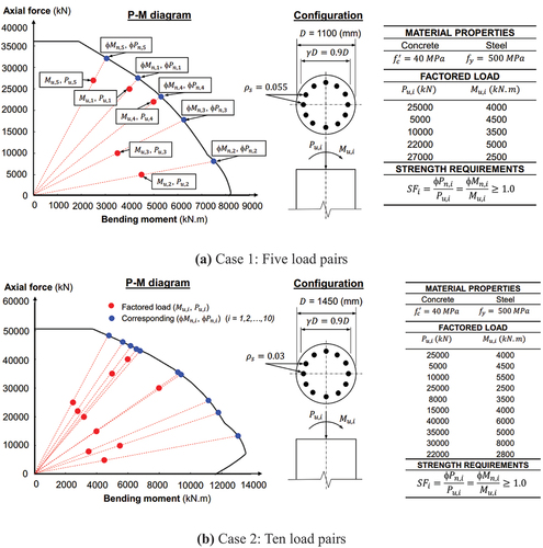
Table 5. ANN-based design Case 1.

Table 6. ANN-based design Case 2.

5.2. Application of hybrid optimization design

Table 5 shows two forward design cases with five and ten load pairs where output parameters are calculated using the preassigned input parameters without optimizations. Table 8 describes the optimized design with five load pairs where column diameters and rebars are optimized by ANN-based Lagrange optimizations. The rebar ratios range from 0.01 to 0.08, which is imposed by the minimum and maximum rebar requirements in the design code ACI 318–19 for RC columns. $\mathit{D}$ is limited between 400 and 2000 mm for its practical applicability. The given factored loads ($P_{\mathit{u},\mathit{i}},\mathit{\hspace{0.17em}}{M}_{\mathit{u},\mathit{i}}$) are five load pairs similar to those in Design Case 1 (Table 5). The preassigned load factors and material properties (steel and concrete) are determined by the equality constraint equations, whereas the limitations of rebar ratio and column diameter are formulated into inequality constraint functions (Table 7). $\mathit{S}{F}_i$ governed by load pair $P_{\mathit{u},\mathit{i}},\mathit{\hspace{0.17em}}{M}_{\mathit{u},\mathit{i}}$ are set as inequalities ($\mathit{S}{F}_i\ge 1.0$) to meet design strength requirements. Figure 5a shows an optimization design in terms of minimizing $\mathit{C}{I}_c$, $\mathit{C}{O}_2$, or $W_c$. The design objective in this example is to minimize cost. An objective function of $\mathit{C}{I}_c$ is derived from the generalized ANNs - Model-LPs. The constraint equations (Table 7) and the objective function are adopted to formulate the Lagrange optimization function. The first-order derivative is implemented, and partial differential equations are linearized before applying the Newton – Raphson method, as discussed in Section 4. Optimal values of $\mathit{D}$ and ${\rho }_s$ are found with respect to the constraint conditions at the input vector ${\mathbf{x}}^{\ast }$ reported during the Lagrange optimization. The output parameters, $\mathit{C}{I}_c$, $\mathit{C}{O}_2$, $W_c$, $\mathit{S}{F}_i$, and ${\epsilon }_{\mathit{s},\mathit{i}}$, corresponding to each load pair are obtained by Model-LPs and calculated by structural mechanics AutoCC to confirm the design accuracies of ANN. $\mathit{D}$ and ${\rho }_s$ are optimized as 1272.8 mm and 0.01, respectively, when the cost $\mathit{C}{I}_c$ is optimized as 225,772 KRW/m based on Lagrange optimization as shown in Table 8. An optimized P-M diagram shown in Figure 5b is plotted based on optimized design results shown in Table 8, in which all load points (red points) are placed inside the optimized P-M diagram. In particular, the $\mathit{S}{F}_i$ are close to 1.0, which indicates an adequate design that is challenging to obtain by the conventional design procedure.

(14) $\underset{[1\times 1]}{\underbrace{\mathrm{y}(C{I}_c)}}=g_{C{I}_c}^{\mathit{D}}\left(f_{\mathit{linear}}\left(\underset{\left[1\times 20\right]}{\underbrace{{\mathit{\omega }}_{C{I}_c}^{(\mathit{out})}}}{f}_{tansig}\left(\underset{\left[20\times 20\right]}{\underbrace{{\mathit{\omega }}_{C{I}_c}^{\left(\mathit{k}\right)}}}\dots f_{tansig}\left(\underset{\left[20\times (2\mathit{n}+4)\right]}{\underbrace{{\mathit{\omega }}_{C{I}_c}^{(1)}}}\underset{\left[(2\mathit{n}+4)\times 1\right]}{\underbrace{{\mathbf{x}}^{(\mathit{in})}}}+\underset{\left[20\times 1\right]}{\underbrace{{\mathbf{b}}_{C{I}_c}^{(1)}}}\right)\dots +\underset{\left[20\times 1\right]}{\underbrace{{\mathbf{b}}_{C{I}_c}^{(\mathit{k})}}}\right)+\underset{\left[1\times 1\right]}{\underbrace{{\mathbf{b}}_{C{I}_c}^{(\mathit{out})}}}\right)\right)$(14)

Figure 5. ANN-based Lagrange optimization.

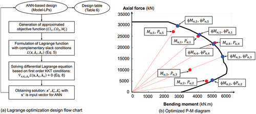
Table 7. Factored load and formulation of inequality and equality constraints.

Equality constraint $\mathit{c}\left(\mathit{x}\right)$	Inequality constraints $\mathit{v}\left(\mathit{x}\right)$
$c_1\left(\mathrm{x}\right)=f_c^{\prime }-40=0$	$v_1\left(\mathit{x}\right)={\rho }_s-0.01\ge 0$
$c_2\left(\mathrm{x}\right)=f_y^{-}500=0$	$v_2\left(\mathit{x}\right)=-{\rho }_s+0.08\ge 0$
$c_3\left(\mathrm{x}\right)=P_{u,1}^{-}25000=0$	$v_3\left(\mathit{x}\right)=\mathit{D}-400\ge 0$
$c_4\left(\mathrm{x}\right)=M_{u,1}^{-}4000=0$	$v_4\left(\mathit{x}\right)=-\mathit{D}+2000\ge 0$
$c_5\left(\mathrm{x}\right)=P_{u,2}^{-}5000=0$	$v_5\left(\mathit{x}\right)=\mathit{S}{F}_1^{-}1.0\ge 0$
$c_6\left(\mathrm{x}\right)=M_{u,2}^{-}4500=0$	$v_6\left(\mathit{x}\right)=\mathit{S}{F}_2^{-}1.0\ge 0$
$c_7\left(\mathrm{x}\right)=P_{u,3}^{-}10000=0$	$v_7\left(\mathit{x}\right)=\mathit{S}{F}_3^{-}1.0\ge 0$
$c_8\left(\mathrm{x}\right)=M_{u,3}^{-}3500=0$	$v_8\left(\mathit{x}\right)=\mathit{S}{F}_4^{-}1.0\ge 0$
$c_9\left(\mathrm{x}\right)=P_{u,4}^{-}22000=0$	$v_9\left(\mathit{x}\right)=\mathit{S}{F}_5^{-}1.0\ge 0$
$c_{10}\left(\mathrm{x}\right)=M_{u,4}^{-}5000=0$
$c_{11}\left(\mathrm{x}\right)=P_{u,5}^{-}27000=0$
$c_{12}\left(\mathrm{x}\right)=M_{u,5}^{-}2500=0$

Table 8. Design table for ANN-based Lagrange optimization.

5.3. Validation of optimized design by large datasets

Five million datasets were generated to validate the optimized design efficiency obtained by a generalized ANN (Model-LPs). Figure 6 shows the contour lines of the objective function ($\mathit{C}{I}_c)$ and $\mathit{S}{F}_i$ values corresponding to five load pairs. $\mathit{D}$ is constrained in a range of 400–2000 mm presented in the x-axis, whereas the y-axis shows the ${\rho }_s$ values. The optimal design identified by brute force method (large datasets) for cost minimization (Table 9) is 228,061 KRW/m, which is 1.01% different from that calculated by ANN Model-LPs. $\mathit{D}$ and ${\rho }_s$ were optimized as 1280 mm and 0.01001, respectively, as indicated in Figure 6. An optimal design lies at a black line indicating that $\mathit{S}{F}_4$ = 1.0, noticeably seen in Figure 6. The acceptable design is located inside a feasible set (Figure 6), demonstrating that all constraint conditions are satisfied. It is noted that any region below $\mathit{S}{F}_4$ = 1.0 is infeasible, while $\mathit{S}{F}_1$ = 1.0, $\mathit{S}{F}_2=\mathit{\hspace{0.17em}}1.0$, $\mathit{S}{F}_3=\mathit{\hspace{0.17em}}1.0$, and $\mathit{S}{F}_5$ = 1.0 are found below $\mathit{S}{F}_4$ = 1.0, indicating that $\mathit{S}{F}_1$, $\mathit{S}{F}_2$, $\mathit{S}{F}_3$, and $\mathit{S}{F}_5$ did not reach 1.0 as shown in Table 8. The optimized design (225,772 KRW/m shown in Table 8) based on ANN-based Lagrange optimization is obtained when ${\rho }_s$ = 0.01 based on KKT condition with active inequality $v_1\left(\mathbf{x}\right)$, and $\mathit{S}{F}_4$ = 1.0 with active inequality $v_8\left(\mathbf{x}\right)$. Other inequalities related to $\mathit{S}{F}_i$ are inactive.

Figure 6. Verification of Lagrange optimization by five million datasets for a P-M diagram capturing five load pairs shown in Figure 5b.

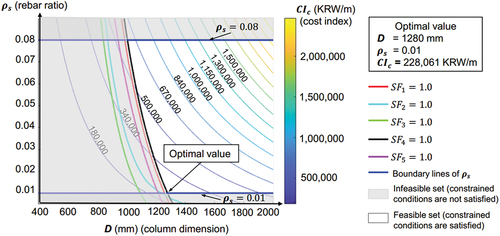
Table 9. Verification of AI-based optimization by large datasets.

Parameters	Model-LPs	Verified by large dataset	Error
CIc (KRW/m)	225,772	228,061	−1.01%
D (mm)	1272.8	1280.0	−0.57%
	0.0100	0.0100	0.00%

Other design parameters are controlled by constraint conditions similar to those with five load pairs for the Lagrange optimization described in Table 8. The $\mathit{S}{F}_i$ in these design examples are controlled within 1.0–1.2 to avoid conservative designs. In Table 10, the cost minimized by ANN-based Lagrange hybrid optimization is compared with a typical cost provided by the probable design of engineers. This probable cost is estimated as the average of 251,496 datasets sorted from five million datasets. Each data in these sorted datasets represents one design completed by each engineer based on a P-M diagram capturing five load points illustrated in Figure 5b. Table 10 compares the probable cost (calculated as 470,508 KRW/m by engineers) and the cost optimized by the Lagrange hybrid design (225,772 KRW/m), which shows a benefit of 51.53% saving.

Table 10. Cost comparison between ANN-based hybrid Lagrange optimization and probable design.

Parameters	Model-LPs	Probable design	Saving
CIc (KRW/m)	225,772	470,508	51.53%

The present study develops the data generating, training, and optimizing codes based on MATLAB Deep Learning Toolbox [MathWorks (2022b)], MATLAB Parallel Computing Toolbox ([MathWorks 2022e]), MATLAB Statistics and Machine Learning Toolbox [MathWorks (2022f)], MATLAB Global Optimization Toolbox [MathWorks (2022c)], MATLAB Global Optimization Toolbox [MathWorks (2022d)], and MATLAB R2022a [MathWorks (2022a)].

6. Summary and conclusions

This study presented an ANN-based modularized weight matrix to design RC round columns capturing multiple load pairs. Cost, CO₂ emission, or weight in the round RC columns was optimized with acceptable accuracies based on a combination of ANN and Lagrange optimization techniques. Their applicability is wide; they are advantageous for round RC columns, and can be applied to any structure, such as beam and frames. This study will aid engineers in making rational design decisions instead of intuitive ones when seeking optimality in their designs. The conclusions drawn from this study are listed below.

1. A design of round concrete column considering one load pair limits the applicability of ANN-based designs, and hence, a generalized ANN (Model-LPs) is proposed to consider multiple load pairs such as multiple factored loads ($P_{\mathit{u},\mathit{i}},M_{\mathit{u},\mathit{i}}$) and their corresponding outputs ($\mathit{S}{F}_i,{\epsilon }_{\mathit{s},\mathit{i}}$). Weight matrices of ANNs are reshaped, preventing re-training of the large datasets. Generation of large structural datasets and training of ANN were performed once with networks considering one load pair, but applied to a design of round concrete column subject to multiple load pairs by duplicating the weight components with respect to $P_u$ and $\mathit{\hspace{0.17em}}{M}_u$in Model-1LP, which leads to a generalized Model-LPs subject to multiple load pairs. The proposed method is to derive networks considering multiple load pairs while removing the needs to re-train networks, contributing to reducing computational time for the practical applications.

2. Lagrange functions are modified to enable an optimization of structural designs to cope with various complex constraint conditions, transforming them into an unbounded optimization problem, which allows derivative methods to be implemented.

3. Cost is minimized by implementing LMM with a generalized ANN (Model-LPs), from which an objective function $\mathit{C}{I}_c$ is extracted while considering multiple load points.

4. Minimized costs accessed by the ANN-based hybrid optimization proposed are validated by those extracted from five million datasets. Besides, design results show negligible errors with those calculated by structural mechanics AutoCC. Designs based on hybrid optimization are significantly beneficial for material savings compared to probable costs by engineers. The cost optimized by the Lagrange hybrid design (225,772 KRW/m) shows a benefit of 51.53% saving compared with the probable cost (calculated as 470,508 KRW/m by engineers). Conservative designs are also avoided by controlling $\mathit{S}{F}_i$ values within 1.0–1.2 in these design examples.

5. Some AI-based structural researches are implemented in specific structures where analytical equations are not available, in which the big data should be collected through experiments. However, the novel holistic ANN-based structural designs for real engineering applications introduced in this study collects big data from structural codes such as ACI, ASCE, AISI, AISE, and EC, etc. directly. All the standards and equations of the codes that are used to generate the big data were already verified by experiments from various researchers. For example, strength reduction factors in ACI 318-19 were established by a study by MacGregor in 1976 [MacGregor, J. G. (1976)], which reviewed test data from multiple studies to develop strength reduction factors, accounting for variabilities in material strengths, overloading, and severities of failure consequences.

Acknowledgements

This work was supported by the National Research Foundation of Korea (NRF) grant funded by the Korean government (MSIT 2019R1A2C2004965).

Disclosure statement

No potential conflict of interest was reported by the author(s).

Additional information

Funding

The work was supported by the National Research Foundation of Korea (NRF) [MSIT 2019R1A2C2004965].

Notes on contributors

Won-Kee Hong

Dr. Won-Kee Hong is a Professor of Architectural Engineering at Kyung Hee University. Dr. Hong received his Master’s and Ph.D. degrees from UCLA, and he worked for Englelkirk and Hart, Inc. (USA), Nihhon Sekkei (Japan) and Samsung Engineering and Construction Company (Korea) before joining Kyung Hee University (Korea). He also has professional engineering licenses from both Korea and the USA. Dr. Hong has more than 30 years of professional experience in structural engineering. His research interests include a new approach to construction technologies based on value engineering with hybrid composite structures. He has provided many useful solutions to issues in current structural design and construction technologies as a result of his research that combines structural engineering with construction technologies. He is the author of numerous papers and patents both in Korea and the USA. Currently, Dr. Hong is developing new connections that can be used with various types of frames including hybrid steel–concrete precast composite frames, precast frames and steel frames. These connections would help enable the modular construction of heavy plant structures and buildings. He recently published a book titled as ”Hybrid Composite Precast Systems: Numerical Investigation to Construction” (Elsevier).

Thuc Anh Le

Thuc Anh Le is currently enrolled as a master candidate in the Department of Architectural Engineering at Kyung Hee University, Republic of Korea. Her research interest includes AI and precast structures.

Manh Cuong Nguyen

Manh Cuong Nguyen is currently enrolled as a master candidate in the Department of Architectural Engineering at Kyung Hee University, Republic of Korea. His research interest includes AI and precast structures.

References

- ACI Committee. 2019. Technical Documents. Farmington Hills, USA: American Concrete Institute.
- Charalampakis, A. E., and V. K. Papanikolaou. 2021. “Machine Learning Design of R/C Columns.” Engineering Structures 226 (March 2020): 111412. https://doi.org/10.1016/j.engstruct.2020.111412.
- Hong, W.-K. 2019. Hybrid Composite Precast Systems (Numerical Investigation to Construction). Alpharetta, USA: Elsevier.
- Hong, W.-K. 2023a. Artificial Neural Network-Based Optimized Design of Reinforced Concrete Structures. Tayor & Francis (CRC press). https://doi.org/10.1201/9781003314684.
- Hong, W.-K. 2023b. Artificial Neural Network-Based Prestressed Concrete and Composite Structures. Milton Park, Abingdon-on-Thames, Oxfordshire United Kingdom: Taylor and Francis.
- Hong, W.-K. 2023c. “(Artificial Neural Networks for Engineering Applications).” In Artificial Intelligence-Based Design of Reinforced Concrete Structures, 329–394. Elsevier. https://doi.org/10.1016/B978-0-443-15252-8.00004-2.
- Hong, W.-K., and M. Cuong Nguyen. 2022. “AI-Based Lagrange Optimization for Designing Reinforced Concrete Columns.” Journal of Asian Architecture & Building Engineering 21 (6): 2330–2344. https://doi.org/10.1080/13467581.2021.1971998.
- Hong, W.-K., M. Cuong Nguyen, and T. Dat Pham. 2022. “Optimized Interaction P-M Diagram for Rectangular Reinforced Concrete Column Based on Artificial Neural Networks Abstract.” Journal of Asian Architecture and Building Engineering 22 (1): null–null. https://doi.org/10.1080/13467581.2021.2018697.
- Hong, W.-K., T. Dat Pham, and V. Tien Nguyen. 2022. “Feature Selection Based Reverse Design of Doubly Reinforced Concrete Beams.” Journal of Asian Architecture and Building Engineering 21 (4): 1472–1496. https://doi.org/10.1080/13467581.2021.1928510.
- Hong, W.-K., T. A. Le, M. C. Nguyen, and T. D. Pham. 2022. “ANN-Based Lagrange Optimization for RC Circular Columns Having Multiobjective Functions.” Journal of Asian Architecture and Building Engineering 22 (2): 961–976. https://doi.org/10.1080/13467581.2022.2064864.
- Hong, W.-K., and M. C. Nguyen. 2021. “AI-Based Lagrange Optimization for Designing Reinforced Concrete Columns.” Journal of Asian Architecture and Building Engineering TABE 21 (6): 2330–2344. https://doi.org/10.1080/13467581.2021.1971998.
- Hong, W.-K., V. T. Nguyen, and M. C. Nguyen. 2021. “Artificial Intelligence-Based Noble Design Charts for Doubly Reinforced Concrete Beams.” Journal of Asian Architecture and Building Engineering 21 (4): 1497–1519. https://doi.org/10.1080/13467581.2021.1928511.
- Kaarthikeyan, K., and D.R.M. Shanthi. 2016. “Optimization of RC Columns Using Artificial Neural Network.” 7 (4): 219–230.
- Lagaros, N. D., and M. Papadrakakis. 2015. “Preface.” Computational Methods in Applied Sciences 38 (c): ix–xii. https://doi.org/10.1007/978-3-319-18320-6.
- Lagrange, J. L. 1804. Leçons sur le calcul des fonctions. Paris: Imperiale.
- MacGregor, J. G. 1976. “Safety and Limit States Design for Reinforced Concrete.” Canadian Journal of Civil Engineering 3 (4): 484–513. https://doi.org/10.1139/l76-055.
- MathWorks, (2022a). MATLAB (R2022a).
- MathWorks, (2022b).” Deep Learning Toolbox: User’s Guide (R2022a).” Accessed July 26, 2012. https://www.mathworks.com/help/pdf_doc/deeplearning/nnet_ug.pdf.
- MathWorks, (2022c). “Global Optimization: User’s Guide (R2022a).” Accessed July 26, 2012. https://www.mathworks.com/help/pdf_doc/gads/gads.pdf.
- MathWorks, (2022d). “Optimization Toolbox: Documentation (R2022a).” Accessed July 26, 2022. https://uk.mathworks.com/help/optim/.
- MathWorks, (2022e). “Parallel Computing Toolbox: Documentation (R2022a).” Accessed July 26, 2022. https://uk.mathworks.com/help/parallel-computing/.
- MathWorks, (2022f). Statistics and Machine Learning Toolbox: Documentation (R2022a). Accessed July 26, 2022. https://uk.mathworks.com/help/stats/.
- Peel, C., and T. K. Moon. 2020. “Algorithms for Optimization [Bookshelf].” IEEE Control Systems 40 (2): 92–94. https://doi.org/10.1109/MCS.2019.2961589.
- Upton, G., and I. Cook. 2014. A Dictionary of Statistics 3e. Oxford university press.
- Villarrubia, G., J. F. De Paz, P. Chamoso, and F. De la Prieta. 2018. “Artificial Neural Networks Used in Optimization Problems.” Neurocomputing 272:10–16. https://doi.org/10.1016/j.neucom.2017.04.075.
- Wang, L., S. Nagarajaiah, W. Shi, and Y. Zhou. 2022b. “Seismic Performance Improvement of Base-Isolated Structures Using a Semi-Active Tuned Mass Damper.” Engineering Structures 271:114963. https://doi.org/10.1016/j.engstruct.2022.114963.
- Wang, L., S. Nagarajaiah, Y. Zhou, and W. Shi. 2023b. “Experimental Study on Adaptive-Passive Tuned Mass Damper with Variable Stiffness for Vertical Human-Induced Vibration Control.” Engineering Structures 280:115714. https://doi.org/10.1016/j.engstruct.2023.115714.
- Wang, L., W. Shi, X. Li, Q. Zhang, and Y. Zhou. 2019a. “An Adaptive‐Passive Retuning Device for a Pendulum Tuned Mass Damper Considering Mass Uncertainty and Optimum Frequency.” Structural Control and Health Monitoring 26 (7): e2377. https://doi.org/10.1002/stc.2377.
- Wang, L., W. Shi, Q. Zhang, and Y. Zhou. 2020a. “Study on Adaptive-Passive Multiple Tuned Mass Damper with Variable Mass for a Large-Span Floor Structure.” Engineering Structures 209:110010. https://doi.org/10.1016/j.engstruct.2019.110010.
- Wang, L., W. Shi, and Y. Zhou. 2019b. “Study on Self‐Adjustable Variable Pendulum Tuned Mass Damper.” The Structural Design of Tall & Special Buildings 28 (1): e1561. https://doi.org/10.1002/tal.1561.
- Wang, L., W. Shi, and Y. Zhou. 2022a. “Adaptive-Passive Tuned Mass Damper for Structural Aseismic Protection Including Soil–Structure Interaction.” Soil Dynamics and Earthquake Engineering 158:107298. https://doi.org/10.1016/j.soildyn.2022.107298.
- Wang, L., W. Shi, Y. Zhou, and Q. Zhang. 2020b. “Semi-Active Eddy Current Pendulum Tuned Mass Damper with Variable Frequency and Damping.” Smart Structures and Systems 25 (1): 65–80. https://doi.org/10.12989/sss.2020.25.1.065.
- Wang, L., Y. Zhou, S. Nagarajaiah, and W. Shi. 2023a. “Bi-Directional Semi-Active Tuned Mass Damper for Torsional Asymmetric Structural Seismic Response Control.” Engineering Structures 293:116744. https://doi.org/10.1016/j.engstruct.2023.116744.
- Wang, L., Y. Zhou, and W. Shi. 2023a. “Seismic Control of a Smart Structure with Semiactive Tuned Mass Damper and Adaptive Stiffness Property.” Earthquake Engineering and Resilience 2 (1): 74–93. https://doi.org/10.1002/eer2.38.
- Wang, L., Y. Zhou, and W. Shi. 2023b. “Seismic Response Control of a Nonlinear Tall Building Under Mainshock-Aftershock Sequences Using Semi-Active Tuned Mass Damper.” International Journal of Structural Stability and Dynamics. https://doi.org/10.1142/S0219455423400278.