A data-driven framework for conceptual cost estimation of infrastructure projects using XGBoost and Bayesian optimization

ABSTRACT

Cost estimation is a key component of project plans, yet it is challenging to provide reliable and efficient estimations using conventional methods in the conceptual phase of infrastructure projects. This study proposes a framework that integrates feature selection, extreme gradient boosting (XGBoost), Bayesian optimization (BO), and SHapley Additive exPlanations (SHAP) to provide conceptual cost estimations and explain the results for early decision-making. Correlation analysis and forward search are combined to select the key features. XGBoost is developed as the estimator and enhanced by BO in accuracy and efficiency. Model explanations were presented using SHAP. The framework is demonstrated through a case study of electric substations containing 605 samples. The results show that the proposed framework can provide satisfactory performance on conceptual cost estimations, where BO-XGBoost outperforms the benchmark models (with $R^2$ ~0.9567, adjusted $R^2$ ~0.9549, RMSE ~ 0.8690, and MAE ~ 0.4875). SHAP reveals how the features contribute to the cost based on both global and local explanations. The framework provides a guideline for more accurate, efficient, and explainable cost estimations in the conceptual phase of infrastructure projects. It can support the government and project planners in early decision-making, including reliable project budget and plan alternatives selection.

KEYWORDS:

• Conceptual cost estimation
• infrastructure
• Xgboost
• Bayesian optimization
• SHAP

1. Introduction

Conceptual cost estimation aims to predict future construction costs by leveraging historical data in the conceptual phase of a project (Diekmann 1983). A conceptual phase refers to the preliminary planning or the predesign phase when a few parameters of a project are available. As a key decision-making element for project planning and execution, accurate conceptual cost estimation is one of the critical factors influencing the success of construction projects (Ahn et al. 2020; Juszczyk 2020).

For infrastructure projects, the objectives of conceptual cost estimation are usually to enable efficient investment decisions (i.e., “GO” or “NO GO” decision) for the government, facilitate the comparison between plan alternatives in terms of their probable costs, and make the construction budget (Hyari, Al-Daraiseh, and El-Mashaleh 2016). However, infrastructure projects frequently experience significant differences between conceptual cost estimations and actual costs in practice (Lee et al. 2022). Inappropriate budgeting based on unreliable and inefficient cost estimation could lead to government financial loss, inefficient project execution, unsatisfied infrastructure quality, and other public relations issues (Bhargava et al. 2017). As infrastructure plays a fundamental role in society and the economy, the success of infrastructure construction closely impacts people’s livelihood and economic growth (Wang et al. 2020). Therefore, the owners and planners of infrastructure projects in the conceptual phase highly desire accurate cost estimations.

Conventionally, the conceptual cost estimation of infrastructure lacks a formal procedure and depends on experts’ own experience, which is often biased and time-consuming (Dursun and Stoy 2016). Indeed, achieving accurate cost estimations in the conceptual phase is challenging. First, the conceptual cost estimations heavily rely on some main features of a project, such as project location and project type (Wang et al. 2022). In contrast, in the design or procurement stage, plenty of design information (i.e., specifications and quantities) can be determined for the detailed cost estimation following the typical cost breakdown structure (CBS) (Ahn et al. 2020; Akanbi and Zhang 2021). Second, the large variety of both infrastructure scopes and equipment usage leads to the smaller quantities of historical samples of infrastructure projects to transfer experience for conceptual cost estimation, which is different from the general construction projects such as residential or office buildings (Lee et al. 2022).

Given these difficulties in the conceptual cost estimation of infrastructure projects, the accuracy of estimation benefits from proper estimation methods. With the increasing awareness of artificial intelligence, cost estimation methods have shifted from conventional methods to machine learning (ML) techniques, which have been acknowledged as promising data-mining tools to address estimation problems by formulating the correlations between the project features and construction cost from learning historical data (Chakraborty et al. 2020; Dursun and Stoy 2016; He, Liu, and Anumba 2021). Based on recent researches, ML has been proven that can minimize human intervention, overcome inaccurate estimations by conventional methods, and often exhibit more satisfactory performance on cost estimation when compared with many other data-mining methods, such as Monte Carlo simulation, Case-based reasoning, time series analysis, fuzzy logic, and multiple linear regression (Cao, Ashuri, and Baek 2018; Elmousalami 2020; Tayefeh Hashemi, Ebadati, and Kaur 2020). Many previous efforts have been made to build ML-based conceptual cost estimation models for different kinds of infrastructures. However, some research limitations in those ML-based applications need to be improved. First, the relatively small-capitalization dataset in the conceptual phase and model efficiency were not considered in the methodology design, which could reduce the accuracy and efficiency of the cost estimation. Second, the study on conceptual cost estimation of infrastructure can go beyond developing a particular estimation model for a certain type of infrastructure, consequently, a conceptual cost estimation framework that can shift the ML utilization in conceptual cost estimation of infrastructure from building a particular ML model to a practical framework is desired.

This study aims to further improve the accuracy and efficiency for the conceptual cost estimation of infrastructure projects, by proposing a BO-XGBoost-based framework. To accomplish this goal, a state-of-the-art ML algorithm, XGBoost, is utilized to build the base estimator, due to its advantages, including (1) higher performance on estimation problems than conventional ML algorithms due to its ensemble technique, (2) good ability to process on relatively small datasets with overfitting prevention. Then, Bayesian optimization (BO) overcomes the inconsistent problem between accuracy and efficiency during hyperparameters tuning, which improves the estimation ability and the efficiency of XGBoost. A multi-step feature selection method is designed to retain features with predictive power before model establishment by integrating correlation analysis, XGBoost, and forward search (FS). SHAP is used to explain the estimation results by revealing how the features contribute to the costs.

The framework is innovative for integrating feature selection, XGBoost, BO, and SHAP to provide more accurate, efficient, and explainable cost estimations in the conceptual phase of infrastructure projects. Therefore, the framework can assist the government and project planners in making reliable budgets and selecting alternative plans.

The remainder of this paper is organized as follows: The related literature is reviewed in Section 2. Then, the methodology is introduced in Section 3. Section 4 demonstrates a BO-XGBoost model in a case study of electric infrastructure with 605 electric substation projects to validate the proposed framework. The model performance and superiority of the proposed BO-XGBoost are analyzed, and SHAP is adopted to explain the estimations by investigating feature contributions. Then, the merits and applicability of the BO-XGBoost-based framework are discussed in Section 5. The main contributions and limitations are presented in the final section.

2. Literature review of machine learning methods in the conceptual cost estimation of infrastructure projects

The reliable cost estimation in the conceptual phase is one of the most crucial criteria for early decision-making in infrastructure projects, which would prevent government financial loss, low-quality construction, and severe project delays (Bhargava et al. 2017). Machine learning methods can make estimations by formulating the potential correlations between the project features and construction cost, even if detailed design information is not available in the conceptual phase. Consequently, there has been a growing awareness among researchers about the applications of machine learning methods to estimate the construction cost in the initial stage of infrastructure projects. Recent studies on this topic are shown in Table 1.

Table 1. Recent studies on conceptual cost estimation of infrastructure projects.

Types	Year	ML models	Number of inputs	Number of samples	Hyperparameter tuning methods	Feature selection methods	Reference
Public construction projects	2016	ANN	5	224	Grid search	Literature, Interviews	(Hyari, Al-Daraiseh, and El-Mashaleh 2016)
Field canal	2018	ANN and MRA	4	144	–	Literature, correlation analysis, and regression	(ElMousalami, Elyamany, and Ibrahim 2018)
Power plant	2019	ANN	9	39	Genetic algorithm	Interviews	(Hashemi, Ebadati, and Kaur 2019)
Bridge	2020	SVM	12	167	Grid search	Based on data availability	(Juszczyk 2020)
Road	2020	ANN	6	57	–	Interviews with experts	(Tijanic, Car-Pusic, and Sperac 2020)
Transportation infrastructure	2020	ANN and MRA	6, 7 and 11	996	–	Interviews, and regression	(Karaca, Gransberg, and Jeong 2020)
Power generation project	2021	ANN and ensemble learning	11	86	–	PCA with MCA	(Lee et al. 2022)
Highway	2022	MLR, ANN, SVM, and ensemble	4	117	Manual tuning	Literature	(Meharie et al. 2022)

ANN: Artificial neural network; SVM: Support vector machine; MRA: Multiple regression analysis; MLR: Multiple linear regression; PCA: Principal component analysis; MCA: multiple correspondence analysis.

The literature listed in Table 1 shows that ML can be a generic method for conceptual cost estimation on various kinds of infrastructure (i.e., power plant, bridge, road, transportation, power generation, and highway). The number of available project features that affect construction cost is often less than 10, and the sample size of historical projects is relatively small (less than 1000). Therefore, the conceptual cost estimation of infrastructure can be considered as a regression problem with relatively small-capitalization dataset, which could result in inaccurate estimations and overfitting problems.

Comprehensive reviews were illustrated from three aspects to investigate how those recent studies deal with the research problem of conceptual cost estimation, including: ML algorithm selection, hyperparameter tuning, and feature selection. Although ML techniques were effective in previous studies, some limitations and defects have remained in these attempts, which may reduce the accuracy, efficiency, and reliability of the estimations for supporting the early decisions of an infrastructure project. More illustrations are as follows:

2.1. ML algorithm selection

ANN was the dominant ML algorithm in previous attempts (Hashemi, Ebadati, and Kaur 2019; Karaca, Gransberg, and Jeong 2020; Tijanic, Car-Pusic, and Sperac 2020). Although ANN overcomes many difficulties presented in conventional regression techniques and linear models, it is extremely data-driven, while the infrastructure dataset in the conceptual phase could be insufficient for ANN training (Tayefeh Hashemi, Ebadati, and Kaur 2020), consequently, reducing the accuracy of the cost estimations and raising the risk of overfitting. Hyari et al (Hyari, Al-Daraiseh, and El-Mashaleh 2016). also reported that the ANN is data intensive, and more project samples are recommended to enhance the reliability of their ANN model. MRA and SVM were investigated in different studies, but no obvious superiority was performed (Juszczyk 2020; Karaca, Gransberg, and Jeong 2020). MRA has also been reported to be weak in formulating complex relationships within cost drivers due to its linear assumptions (Elmousalami 2020). In recent years, ensemble learning has become the next-generation cost estimation technique. It combines a series of individual base learners to improve the overall estimation in terms of accuracy and stability, and can achieve better accuracy than any single base learner (Meharie et al. 2022). Therefore, although the performance of ML is often affected by the size of datasets, ensemble learning is desired to outperform the conventional ML methods to process insufficient datasets by continuously integrating the base learners. Lee et al (Lee et al. 2022), Meharie et al (Meharie et al. 2022). conducted ensemble modeling to enhance their base learners (such as ANN, MLR, or SVM), and achieved good estimation accuracy for different types of infrastructures. However, considering the relatively small size of the infrastructure dataset, some state-of-the-art ensemble learning algorithms could be more suitable for the conceptual cost estimation than directly using ensemble modeling to integrate a series of ML models. For example, XGBoost has been highlighted to have strong ability to generate reliable estimation models (Almasabha et al. 2023), and have high performance in the construction field, such as residual value prediction for heavy construction equipment (Shehadeh et al. 2021), disability status prediction for construction workers (Koc, Ekmekcioglu, and Gurgun 2021), impact evaluation of external support on green building construction cost (Alshboul et al. 2022), and proactive damage estimation for bridges (Lim and Chi 2019).

2.2. Hyperparameter tuning

Second, hyperparameter tuning is a critical process to determine the ML model configurations during model training. The model performance relies heavily on appropriate combinations of the hyperparameters. However, the tuning processes are not mentioned in some studies (Karaca, Gransberg, and Jeong 2020; Lee et al. 2022; Tijanic, Car-Pusic, and Sperac 2020). Meharie et al. (2022). applied the manual tuning method to determine the hyperparameters of their ML models. Manual tuning is a trial-error process based on the users’ experience, with the drawbacks of tedious processes and unreliable tuning results (Kim et al. 2022). Juszczyk (2020), (Hyari, Al-Daraiseh, and El-Mashaleh 2016). selected grid search (GS), which is the most widely used hyperparameter tuning method based on the exhaustive searching principle (Wu et al. 2019). However, GS suffers from the limitation of candidate dimensionality since it evaluates every combination of hyperparameter candidates. The time consumption of GS increases exponentially when the number of hyperparameter candidates increases, which means that the expensive computational cost of GS causes a deficiency in the accuracy-efficiency balance (Wu et al. 2019). Hashemi, Ebadati, and Kaur (2019). used a metaheuristic algorithm named genetic algorithm (GA) to find the near-optimal hyperparameters for their ANN model. Although the GA can avoid the local optima problem, the parameters of its basic operators are often determined by users’ experience, while inappropriate parameters decrease the GA performance significantly.

With regard to the conceptual cost estimation in construction practice, Bayesian optimization (BO) was recently proven efficient in achieving the global optimal hyperparameters for ML models (Kim et al. 2022). BO obtains the optimal hyperparameters without evaluating all the combinations of hyperparameters, which can reduce the training time significantly on model development and improve both the accuracy and efficiency of cost estimation using ML.

2.3. Feature selection

Third, the performance of the ML model is also affected by the input features since the redundant features would mislead ML models in learning the historical samples. Selecting the features with predictive power from the collected data becomes more essential when the sample size is relatively small (Huang, Li, and Xie 2015). Based on Table 1, qualitative methods, such as literature, surveys, and interviews with experts, are the most common and convenient methods to determine the input features due to the small data size in the conceptual phase (Hashemi, Ebadati, and Kaur 2019; Hyari, Al-Daraiseh, and El-Mashaleh 2016; Juszczyk 2020; Meharie et al. 2022; Tijanic, Car-Pusic, and Sperac 2020). However, these studies single used the qualitative method, which may overlook both the correlations within the features and the features’ real effects on the costs. Since qualitative methods lack deep statistical analysis for ML to understand the dataset, some scholars combined quantitative methods, such as factor analysis, correlation analysis, and regression methods with qualitative methods for more reliable feature selection (ElMousalami, Elyamany, and Ibrahim 2018; Karaca, Gransberg, and Jeong 2020; Lee et al. 2022). The reviewed literature shows that factor analysis (i.e., PCA) and correlation analysis can efficiently eliminate some redundant features. However, a single factor analysis or correlation analysis is often insufficient for feature selection, and weak in providing causality to interpret the features (Elmousalami 2020). Regression analysis can be effective for both feature selection and cost estimation modeling, since regression models can evaluate how much each feature influences the model performance by adjusting the input features stepwise (Mohsenijam, Siu, and Lu 2017). ElMousalami et al (ElMousalami, Elyamany, and Ibrahim 2018), Karaca et al (Karaca, Gransberg, and Jeong 2020). combined qualitative methods and regression methods based on MRA for feature selection, while MRA may not be the most suitable model for conceptual cost estimation, as mentioned in Section 2.1. Due to the small data size in the conceptual cost estimation of infrastructure projects, more attention could be paid to feature selection to check the predictive power of the model’s inputs.

2.4. Research gaps

The literature review demonstrates work that conducted the conceptual cost estimation in infrastructure projects using various machine learning methods. The evidence shows that machine learning methods can be effective decision-support tools in construction practice. However, the size of the dataset and overfitting issues were seldom considered when selecting the ML algorithms, which would reduce the reliability of the estimation results. Then, many studies paid little attention to hyperparameter tuning, which may limit both the accuracy and efficiency of the ML-based cost estimations to a large extent. In some studies, an absence of a considerable feature selection process may mislead the model estimations due to redundant features. Furthermore, earlier studies seldom explained their ML models by linking the results of cost estimations and feature importance, which could lose some valuable information for supporting early decision-making.

Therefore, further studies are expected to integrate thoughtful feature selection and hyperparameter tuning methods to the appropriate ML algorithm utilization against the overfitting issues in the conceptual cost estimation of infrastructure projects, which can provide satisfactory, efficient, and reliable estimations.

This study provides a guideline framework on the conceptual cost estimations of infrastructure projects for providing satisfactory, efficient, and reliable estimation results. The paradigm and findings can also give the government and project planners valuable insights into explainable machine learning and feature importance to support early decision-making in infrastructure projects.

3. Methodology

3.1. Machine learning techniques

3.1.1. Extreme gradient boosting (XGBoost)

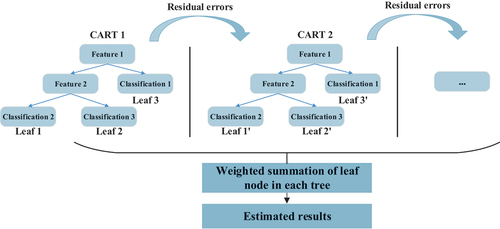
XGBoost is a tree-based ensemble learning algorithm proposed by Chen and Guestrin in 2016 (Chen, Guestrin, and Assoc Comp 2016) to solve classification and regression tasks. It integrates a series of base learners (classification and regression trees, CARTs) to build a robust estimator with optimal model performance.

As mentioned in Section 2.1, ensemble learning methods are becoming the next-generation cost estimation techniques to deal with relatively small-size datasets. Considering the relatively small-capitalization project sample size in the conceptual cost estimation of infrastructure projects, XGBoost is an appropriate ensemble learning algorithm to provide accurate cost estimations for two reasons. First, XGBoost often exhibits state-of-the-art performance and outperforms many ML algorithms on various estimation problems, with high accuracy and model robustness (Koc, Ekmekcioglu, and Gurgun 2021; Lim and Chi 2019). Second, compared with many conventional ML algorithms, deep learning algorithms, and other ensemble learning methods, XGBoost can not only work well on large dataset, but also has a stronger ability to process relatively small datasets and prevent overfitting since a regularization function is added to its objective function (Dong et al. 2020; Lv et al. 2020; Zhang et al. 2019). In addition, XGBoost has minimal requirements for data normalization (Dong et al. 2020) and data diversity (Almasabha et al. 2023), which can benefit its applicability in real construction practice.

The schematic of XGBoost is to successively add and train new CARTs based on residual errors of the last iteration, as shown in Figure 1. The final estimation value is the sum of all the continuous scores in the CART leaves, the estimated value of an infrastructure cost $\hat{y}$ is expressed as Equation 1(1) $\hat{y}=\sum _{k=1}^K{f}_k\left(x_i\right),f_k\in F$(1) (Chen, Guestrin, and Assoc Comp 2016):

Figure 1. Schematic of XGBoost (Huang and Meng 2019).

(1) $\hat{y}=\sum _{k=1}^K{f}_k\left(x_i\right),f_k\in F$(1)

where $f_k$ denotes the independent tree structure of the k-th CART; $f_k\left(x_i\right)$ is the estimated score of the k-th CART using the i-th project sample; $K$ stands for the number of additive CARTs; and $F$ is the whole space composed of all the CARTs. The model estimation improves based on the residual error of the previous CART in each iteration (Huang and Meng 2019), as shown in Figure 1. The objective function of the model is composed of the loss function and regularization function, as shown in Equation 2(2) $J\left(t\right)=\sum _{i=1}^{n}l\left(y_i,{\hat{y}}_i\right)+\sum _{k=1}^K\mathrm{\Omega }\left(f_k\right)=\sum _{i=1}^{n}l\left(y_i,{\hat{y}}_i^{\left(t-1\right)}+f_t\left(x_i\right)\right)+\sum _{k=1}^K\mathrm{\Omega }\left(f_k\right)+constant$(2) :

(2) $J\left(t\right)=\sum _{i=1}^{n}l\left(y_i,{\hat{y}}_i\right)+\sum _{k=1}^K\mathrm{\Omega }\left(f_k\right)=\sum _{i=1}^{n}l\left(y_i,{\hat{y}}_i^{\left(t-1\right)}+f_t\left(x_i\right)\right)+\sum _{k=1}^K\mathrm{\Omega }\left(f_k\right)+constant$(2)

where $l$ is the loss function to calculate the loss value between the estimated cost $y_i$ of the i-th sample at the t-th iteration and the estimated cost ${{\hat{y}}_i}^{\left(t-1\right)}$ at the (t-1)-th iteration; $f_t\left(x_i\right)$ is a new CART to form the t-th tree; and $\mathrm{\Omega }$ is the regularization function to penalize the model complexity for each tree, which aims to avoid overfitting, as shown in Equation 3(3) $\mathrm{\Omega }\left(f_k\right)=\gamma T+\frac{1}{2}\lambda \sum _{j=1}^T{\omega }_j^2$(3) :

(3) $\mathrm{\Omega }\left(f_k\right)=\gamma T+\frac{1}{2}\lambda \sum _{j=1}^T{\omega }_j^2$(3)

Here $\omega$ denotes the score of each leaf node; $T$ is the quantity of leaf nodes; $\gamma$ is a penalty coefficient corresponding to the model complexity of the newly added nodes; and $\lambda$ is another penalty parameter to avoid overfitting. Second-order Taylor expansion is used to efficiently optimize the loss function in Equation 2(2) $J\left(t\right)=\sum _{i=1}^{n}l\left(y_i,{\hat{y}}_i\right)+\sum _{k=1}^K\mathrm{\Omega }\left(f_k\right)=\sum _{i=1}^{n}l\left(y_i,{\hat{y}}_i^{\left(t-1\right)}+f_t\left(x_i\right)\right)+\sum _{k=1}^K\mathrm{\Omega }\left(f_k\right)+constant$(2) . The objective function $J\left(t\right)$ is approximated as Equation 4(4) $J\left(t\right)\simeq {\sum }_{i=1}^n\left[l\left(y_i,{\hat{y}}_i^{\left(t-1\right)}\right)+g_i{f}_t\left(x_i\right)+\frac{1}{2}{h}_i{f}_t^2\left(x_i\right)\right]+\mathrm{\Omega }\left(f_t\right)+constant$(4) :

(4) $J\left(t\right)\simeq {\sum }_{i=1}^n\left[l\left(y_i,{\hat{y}}_i^{\left(t-1\right)}\right)+g_i{f}_t\left(x_i\right)+\frac{1}{2}{h}_i{f}_t^2\left(x_i\right)\right]+\mathrm{\Omega }\left(f_t\right)+constant$(4)

where $g_i=\mathrm{\partial }{\hat{y}}^{\left(t-1\right)}l\left(y_{i,}{\hat{y}}^{\left(t-1\right)}\right)\mathrm{a}\mathrm{n}\mathrm{d}{h}_i=\mathrm{\partial }{ }^2{\hat{y}}^{\left(t-1\right)}$ $l\left(y_i,{\hat{y}}^{\left(t-1\right)}\right)$ are the first-order and second-order derivatives of the loss function, respectively. The constant term can be removed to further simplify the objective function, as shown in Equation 5(5) $J\left(t\right)\simeq \sum _{i=1}^n[g_i{f}_t\left(x_i\right)+\frac{1}{2}{h}_i{f}_t^2\left(x_i\right)]+\gamma T$(5) :

(5) $J\left(t\right)\simeq \sum _{i=1}^n[g_i{f}_t\left(x_i\right)+\frac{1}{2}{h}_i{f}_t^2\left(x_i\right)]+\gamma T$(5)

then, $I_j=\left\{i|q\left(x_i\right)=j\right\}$ is defined as the set of infrastructure project features assigned to leaves $j$ in tree structures. Defining $G_j=\sum _{i\in I_j}{g}_i$, $H_j=\sum _{i\in I_j}{h}_i$. Therefore, the objective function can be rewritten to reveal the ergodicity of all leaf nodes, as shown in Equation 6(6) $J\left(t\right)=\sum _{j=1}^T\left[\left(\sum _{i\in I_j}{g}_i\right){\omega }_j+\frac{1}{2}\left(\sum _{i\in I_j}{h}_i+\lambda \right){\omega }_j^2\right]+\gamma T=\sum _{j=1}^T\left[G_j{\omega }_j+\frac{1}{2}{H}_j{\omega }_j^2\right]+\gamma T$(6) :

(6) $J\left(t\right)=\sum _{j=1}^T\left[\left(\sum _{i\in I_j}{g}_i\right){\omega }_j+\frac{1}{2}\left(\sum _{i\in I_j}{h}_i+\lambda \right){\omega }_j^2\right]+\gamma T=\sum _{j=1}^T\left[G_j{\omega }_j+\frac{1}{2}{H}_j{\omega }_j^2\right]+\gamma T$(6)

When the tree structure $q\left(x_i\right)$ is fixed, the optimal weight ${\omega }_j^{\ast }$ of leaf j can be determined in Equation 7(7) ${\omega }_j^{\ast }=-\frac{G_j}{H_j+\lambda }$(7) , and the new objective function is derived as shown in Equation 8(8) $J\left(t\right)=-\frac{1}{2}{\sum }_{j=1}^T\frac{{G_j}^2}{H_j+\lambda }+\gamma T$(8) :

(7) ${\omega }_j^{\ast }=-\frac{G_j}{H_j+\lambda }$(7)

(8) $J\left(t\right)=-\frac{1}{2}{\sum }_{j=1}^T\frac{{G_j}^2}{H_j+\lambda }+\gamma T$(8)

3.1.2. Gradient boosting decision tree (GBDT)

Gradient boosting decision tree (GBDT) is another powerful ensemble learning algorithm based on the decision tree. Similar to XGBoost, GBDT also adopts the boosting strategy that combines a series of weak learners (i.e., CART) to form a strong predictor to minimize the loss function by iteration (Gu et al. 2021). Compared with XGBoost, the training of GBDT is based on the idea of gradient descent. In this process, each CART is trained from the residuals of the previous one to fit the negative gradient of the loss function (Rao et al. 2019). Another major difference is that the regularization function is not added to GBDT’s objective function. The steps of GBDT are as follows (Gu et al. 2021):

(1) Initializing the weak learner (CART):

(9) $f\left(x\right)=argmi{n}_e\sum _{i=1}^{N}L\left(y_i,e\right)$(9)

where $L\left(y_i,e\right)$ is the loss function, $y_i$ is the real construction cost of an infrastructure project, $e$ is the estimated cost, $N$ is the sample size.

(2) Calculating the negative gradient of the loss function $L$ in each iteration m (1,2 … M):

(10) $g_{nm}=-{\left[\frac{\mathrm{\partial }L\left(y_i,f\left(x_n\right)\right)}{\mathrm{\partial }f\left(x_n\right)}\right]}_{f\left(x\right)-f_{m-1}\left(x\right)}$(10)

where M is the number of iterations, n = 1,2 … N.

(3) Fitting the residual of a CART $h_m\left(x\right)$ by minimizing the loss,

(4) Calculate optimal fitting value:

(11) $e_m=argmi{n}_e\sum _{i=1}^{N}L\left(y_i,f_{m-1}\left(x\right)+e{h}_m\left(x\right)\right)$(11)

(5) Updating the model:

(12) $f_m\left(x\right)=f_{m-1}\left(x\right)+e_m{h}_m\left(x\right)$(12)

(6) Repeating Steps (2) - (5) to get the final GBDT model:

(13) $f\left(x\right)=\sum _{m=1}^M{e}_m{h}_m\left(x\right)$(13)

3.1.3. Artificial neural network (ANN)

As reviewed in section 2, artificial neural network (ANN) is a popular algorithm in previous studies on conceptual cost estimations. Back propagation neural network (BPNN) is a kind of ANN that has been widely utilized in prediction problems due to its good nonlinear fitting ability (Bai et al. 2021).

BPNN is a feed-forward neural network trained according to the back propagation algorithm to train the model. It is designed as a multilayer structure that consists of an input layer, one or more hidden layers, and an output layer. The layers are connected by numerous nodes. The learning process of BPNN is divided into forward propagation and error backpropagation: (1) the training data flows forward from the input layer to the output layer. The weights and thresholds are trained to minimize the error between the estimation and the desired result. An activation function is to map the output signal to the next layer. (2) Based on the gradient descent method, if the error exceeds the expectation, the gradient signal is fed back into the neural network in a back propagation process to correct the weight and bias, and minimize the error between the estimated values and actual values (Zhou et al. 2023). In the network, the output value of a node $y_i$ when given the input $x_j$ is represented as follows (Zhou et al. 2023):

(14) $y_i=f\left(\sum _{j=1}^n{w}_{ij}{x}_j+b_i\right)$(14)

where $w_{ij}$ is the weight of the node between nodes i and j, $b_i$ is the bias of the node i, f(x) is the activation function

3.1.4. Support vector regression (SVR)

Support vector regression (SVR) is a form of support vector machine (SVM) that is widely used for handling regression tasks (Beniwal, Singh, and Kumar 2023). The principle of SVR is to map the features into high-dimensional space, and find a hyperplane to separate the samples while minimizing the error margin of the SVR function f(x). The hyperplane is determined by selecting a suitable kernel function that involves linear, polynomial, and RBF kernel function. The function f(x) is defined as (Son, Kim, and Kim 2012):

(15) $f\left(x\right)=w\ast \mathrm{\varnothing }\left(x\right)+b$(15)

where f(x) represents the estimated cost in the current study, w is the weight vector, $\mathrm{\varnothing }$ is the nonlinear map, b is the bias term.

Then, the SVR is to find the optimal values of w and b that minimize the error between the estimated costs and the actual costs. Therefore, the goal of SVR can be defined as (Mahmoodzadeh, Nejati, and Mohammadi 2022):

(16) $\mathrm{m}\mathrm{i}\mathrm{n}\mathrm{i}\mathrm{m}\mathrm{i}\mathrm{z}\mathrm{e}\frac{1}{2}||w||{ }^2+C\ast \sum _{i=1}^m\left(\xi +{\xi }_i^{\ast }\right)$(16)

subject to:

$y-f\left(x\right)\le \epsilon +{\xi }_i$

$f\left(x\right)-y\le \epsilon +{\xi }_i^{\ast }$

${\xi }_i,{\xi }_i^{\ast }\ge 0$

where y is the actual output value, C is a regularization constant that controls the trade-off between regression and penalized loss, ɛ is the width of the insensitive zone that defines the width of the margin. ${\xi }_i$ and ${\xi }_i^{\ast }$ are the slack variables to measure the deviation between y and f(x) from the boundary’s extension area, which is used to penalize the samples for being misclassified on the incorrect side of the hyperplane.

3.1.5. Multiple linear regression (MLR)

Multiple linear regression (MLR) is an effective model in the literature to formulate the relationship between independent variables and a dependent variable to estimate the construction cost (Meharie et al. 2022). MLR has low complexity to execute, and can provide good performance when the relationship between the independent and target variables is linear. The basic principle is linear regression, when there is only one independent variable and one target variable. MLR is the multivariate analysis of linear regression when investigating more than one independent variable (Mahmoodzadeh, Nejati, and Mohammadi 2022), which can be described in Equation 17(17) $y_i={\beta }_0+{\beta }_1{x}_1+{\beta }_2{x}_2+{\beta }_3{x}_3+\dots {\beta }_n{x}_n+\epsilon$(17) .

(17) $y_i={\beta }_0+{\beta }_1{x}_1+{\beta }_2{x}_2+{\beta }_3{x}_3+\dots {\beta }_n{x}_n+\epsilon$(17)

where y is the estimated construction cost in the present study, x is each input feature, ${\beta }_0$ is a constant term of the y intercept, ${\beta }_n$ is the slope coefficient of each feature, $\epsilon$ is an error term.

3.2. Hyperparameters tuning method: Bayesian optimization (BO)

In this study, Bayesian optimization (BO) is employed for XGBoost hyperparameter tuning. An optimal combination of hyperparameters can directly influence the ML model performance. As mentioned in Section 2, the conventional hyperparameter tuning methods have the shortcomings of high time consumption and low efficiency. Since many hyperparameters can be tuned in XGBoost, optimizing an XGBoost could cost much time using conventional methods (i.e., GS), which is not desired in early decision-making. To address this problem, BO is an efficient and effective method to optimize an expensive black-box function, and has gradually been used in hyperparameter tuning for ML models to eliminate the inconsistency problem between accuracy and efficiency (Luong et al. 2021). Previous studies have also proven that BO can achieve better optimization outcomes and much higher efficiency than other conventional methods, especially when there are many hyperparameters that need to be optimized (Shi et al. 2021).

The objective function of hyperparameter tuning is unknown and often with expensive computation (Shi et al. 2021). The concept of BO is derived from Bayes’ rule, which utilizes the prior information to predict the posterior possibility, as shown in Equation 18(18) $p\left(f|D\right)=\frac{p(D|f)p\left(f\right)}{p\left(D\right)}$(18) (Shin et al. 2020):

(18) $p\left(f|D\right)=\frac{p(D|f)p\left(f\right)}{p\left(D\right)}$(18)

where f is the objective function, D is the quantity of prior sampled hyperparameters, p(D) denotes the prior distribution of f, p(D|f) is the likelihood at a sampling point, and p(f|D) represents the posterior distribution of f.

BO takes advantage of the prior distribution of objective function f(x) from the sampled hyperparameters, and continuously updates the posterior distribution to select the new sampling point of the hyperparameter combinations (Shahriari et al. 2016). Hence, BO can efficiently find the direction of optimization based on prior experience without searching through all the hyperparameter samples.

In the BO process, a surrogate model and an acquisition function $\alpha \left(x\right)$ are the two core components. The surrogate model is to predict the objective function f(x) at sampling point x by considering the prior distribution based on a Gaussian process (GP) (Vasconcelos et al. 2022). GP is the most common probabilistic model that acts as a surrogate model for Bayesian optimization due to its high flexibility. Gaussian process over function f(x) is denoted as (Vasconcelos et al. 2022):

(19) $f\left(x\right)\sim GP\left(m\left(x\right),k\left(x_i,x_j\right)\right)$(19)

where the mean function m:$x\to$ℝ, and the covariance function k:$x\times x\to$ℝ.

The acquisition function is responsible for selecting the next sampling point with the consideration of GP. The acquisition function balances exploration and exploitation when sampling (Wu et al. 2019), which influences the efficiency of hyperparameter optimization. Exploration is to sample in a region with high uncertainty where there are few prior sampling points, and exploitation is to sample in the region where model prediction has already been good based on the posterior distribution. Expected improvement (EI) is one of the acquisition functions and employed in this study. EI calculates the expectation of the improvement at a sampling point when exploiting (Shi et al. 2021), which means it will shift to explore a new sampling point in other areas when the improvement of function f(x) is less than the expectation. Therefore, EI has a strong ability to avoid falling into the local optimal solution (Shahriari et al. 2016; Vasconcelos et al. 2022). Compared with the value of the current optimum sampling point $y^{+}$, if the improvement of f(x) is greater than the expectation, the EI result is positive; otherwise, it is 0. Hence, EI is expressed as (Shahriari et al. 2016; Vasconcelos et al. 2022):

(20) $EI\left(x\right)=\left(\mu \left(x\right)-x\left(x^{+}\right)\right)\Phi \left(z\right)+\sigma \left(x\right)\varphi \left(z\right)if\sigma \left(x\right)00if\sigma \left(x\right)=0$(20)

where $\mu \left(x\right)$ and $\sigma \left(x\right)$ are the posterior predictions from the GP, and $z=\frac{\mu \left(x\right)-y^{+}}{\sigma \left(x\right)}$, $\mathrm{\Phi }$ and $\varphi$ are the cumulative density function (CDF) and probability density function (PDF) of the standard Gaussian distribution, respectively.

3.3. The proposed BO-XGBoost-based framework

The primary goal is to propose a framework for providing more accurate, efficient, and explainable cost estimations in the conceptual phase of infrastructure projects. Based on Sections 3.1 and 3.2, a BO-XGBoost-based framework is proposed for the conceptual cost estimation, as shown in Figure 2. The framework consists of data collection and preparation, multi-step feature selection, model establishment, performance evaluation, and model interpretability. In this framework, feature selection integrates correlation analysis, forward search (FS), and XGBoost. During model establishment, the XGBoost is trained and improved via BO. Afterward, the model performance and feature importance are analyzed.

Figure 2. The BO-XGBoost-based framework.

3.3.1. Data collection and preparation

The data of both independent and dependent variables should be collected before the BO-XGBoost model establishment. Due to the small data size in the conceptual phase, the initial cost-related features can be identified based on both experts’ experience and literature as independent variables. Based on the previous studies and the definition of conceptual cost estimation by the Association for the Advancement of Cost Estimation (AACE), the known features with predictive power in the conceptual phase are often little more than the project location, project type, and capacity (AACE 2004). The dependent variable is the construction cost at the end of the completion stage.

Data encoding aims to convert the features with categorical data into numerical data, since numerical data are more acceptable for ML model development (Xue et al. 2019). Label encoding approach is adopted since it can efficiently map categorical data into specific numeric and guarantee a smooth modeling process without an increase in the data dimension (Koc, Ekmekcioglu, and Gurgun 2021).

3.3.2. Multi-step feature selection

The purpose of feature selection is to control the quality of the model’s inputs, especially when the sample size is relatively small. It removes the redundant features in the initial dataset, and retains the features with the predictive power for improving estimation accuracy. Otherwise, the redundant features can mislead the model training, cause the overfitting problem, and degenerate the model performance (Mahmoodzadeh, Nejati, and Mohammadi 2022). As mentioned in Section 2.3, the regression method has been proven effective for feature selection. In this study, XGBoost regression and forward search (FS) are integrated along with the correlation analysis for feature selection as shown in Figure 2. The multi-step feature selection is designed as below:

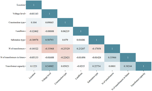
Step 1: Correlation analysis is effective and widely used for feature selection to filter out irrelevant or redundant features. In the current study, the Spearman rank correlation coefficient is calculated to examine the correlations between each pair of features. This method is used to filter out some redundant features with strong inter-correlation. The value of the correlation coefficient ranges from 1 to −1, and a value of 0 indicates no correlation between the pair of variables. If the absolute value of the correlation coefficient is close to 1, a strong correlation exists between the pair of variables (Shehadeh et al. 2021). Redundancy may be hidden between two independent variables if they have a strong correlation.

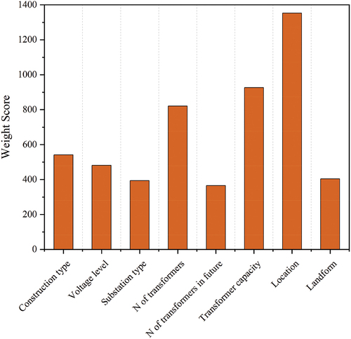
Step 2: XGBoost can provide “weight” score that measures each feature’s contribution to the XGBoost establishment. Since XGBoost selects suitable features at the tree split points during the training process (Shi et al. 2021), the “weight” score means the number of times a feature is selected at the splitting nodes in all generated trees. Therefore, “weight” score has been used to test the feature’s contribution regarding XGBoost establishment (Guo et al. 2019; Liu et al. 2021). A very low “weight” score indicates that the feature is seldom used to establish the XGBoost model.

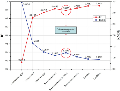
Step 3: The XGBoost-based FS is conducted to evaluate the performance improvement contributed by each feature. Although correlation analysis is an effective method in feature selection, a single use of correlation analysis is inadequate to remove the redundant feature. FS can directly examine the real effect of each feature on the target variable (Guo et al. 2019). The FS process starts with no input feature to an XGBoost regression model. Then, each candidate feature is imported to XGBoost sequentially (Mohsenijam, Siu, and Lu 2017). In each iteration, the estimation result is measured after 5-fold cross-validation (explained in Section 3.3.3) to evaluate whether the imported feature can improve the estimation accuracy according to the coefficient of determination ($R^2$) and root mean square error (RMSE). If an imported feature has predictive power to improve the estimation accuracy, it is selected and retained for BO-XGBoost establishment, otherwise, the feature is removed. After the first imported feature has been evaluated, FS method searches for a second input feature in next iteration. This iteration is repeated until all the features have been evaluated.

3.3.3. Model establishment

As shown in Figure 2, the establishment of the BO-XGBoost consists of 3 steps:

Step 1: Defining the initial hyperparameters of XGBoost. Since BO aims to find the optimal combination of the hyperparameters of XGBoost, the name and initial values of the hyperparameters determine the BO sampling domain of exploration and exploitation. The hyperparameters can include learning_rate, max_depth, min_child_weight, n_estimators, reg_alpha, and gamma.

Step 2: Training the XGBoost model. The database is divided into a training set and a test set. K-fold cross validation is employed to support model training and assess training results. Using the K-fold cross validation, the training set is randomly partitioned into k equal subsets called folds, and the XGBoost model is trained for k times in each iteration of BO. Each time, (k-1) folds are selected for model training, while the remaining folds are used as validation set simultaneously (Shehadeh et al. 2021). Therefore, the optimal hyperparameter combination with the highest average performance among the k-fold subsets is selected. By this means, the data dependency can be minimized, which prevents overfitting and improves the reliability of the training results (Son, Kim, and Kim 2012). In the present study, 5-fold cross validation is implemented on model training. The initial XGBoost model is developed with the hyperparameters defined in step 1, and the training process follows Equation 1(1) $\hat{y}=\sum _{k=1}^K{f}_k\left(x_i\right),f_k\in F$(1) - Equation 8(8) $J\left(t\right)=-\frac{1}{2}{\sum }_{j=1}^T\frac{{G_j}^2}{H_j+\lambda }+\gamma T$(8) . The test set is used for evaluating the estimation accuracy finally.

Step 3: Optimizing the hyperparameters of XGBoost by BO. Step 3 is implemented parallel to step 2. Based on section 3.2, GP acts as a probabilistic model of the prior hyperparameter sampling results, and the acquisition function EI selects the next sample values of the combination of hyperparameters. In each time the BO finds a suitable combination of hyperparameters, a 5-fold cross validation is executed to evaluate the average performance of the hyperparameters on the 5 validation sets. This process is repeated to find better hyperparameters during model training until the preset number of iterations is reached, so as to optimize the objective function of XGBoost. Once the iteration is stopped, the optimal combination of the BO-XGBoost hyperparameters is retained, which contributes to the final BO-XGBoost model.

3.3.4. Model performance evaluation

This study measures the model performance via four extensively used statistical metrics for ML models, including: $R^2$, RMSE, mean absolute error (MAE) and adjusted $R^2$. These metrics are calculated by comparing the estimated and actual costs, as shown in Equation 21(21) $R^2=1-\frac{{\sum }^{{\left(y_i-{\hat{y}}_i\right)}^2}}{{\sum }^{{\left(y_i-\bar{y}\right)}^2}}$(21) to Equation 24(24) $Adjusted{R}^2=1-\left(\frac{\left(1-R^2\right)\times \left(n-1\right)}{\left(n-p-1\right)}\right)$(24) .

The coefficient of determination $R^2$ indicates the percentage of the square of the correlation between the estimated and actual values. It characterizes the degree of regression fitting on all the investigated samples, and is often adopted as the main metric to assess the prediction accuracy of regression problems (Shehadeh et al. 2021), which is defined as:

(21) $R^2=1-\frac{{\sum }^{{\left(y_i-{\hat{y}}_i\right)}^2}}{{\sum }^{{\left(y_i-\bar{y}\right)}^2}}$(21)

To support $R^2$ results, RMSE and MAE are given as:

(22) $RMSE=\sqrt{\frac{1}{n}\sum _{i=1}^n{\left(y_i-{\hat{y}}_i\right)}^2}$(22)

(23) $MAE=\frac{1}{n}\sum _{i=1}^n\left|\left(y_i-{\hat{y}}_i\right)\right|$(23)

The adjusted $R^2$ (Equation 16) penalizes the number of input features to adjust the potential overfitting in $R^2$ (Elmousalami 2020).

(24) $Adjusted{R}^2=1-\left(\frac{\left(1-R^2\right)\times \left(n-1\right)}{\left(n-p-1\right)}\right)$(24)

where n represents the number of instances, $y_i$ denotes the observed cost, ${\hat{y}}_i$ represents the estimated cost, $\bar{y}$ stands for the mean value of the estimated cost, and $p$ denotes the number of features. Based on the principles of those metrics, higher values of $R^2$ and adjusted $R^2$ and lower values of RMSE and MAE indicate higher accuracy.

3.3.5. Model interpretability

Model interpretability aims to dig out more valuable information behind the estimation results and support decision-making in practice. Shapley Additive exPlanations (SHAP), as a powerful “Explainable Artificial Intelligence (XAI)” technique designed by Lundberg and Lee in 2017 (Lundberg and Lee 0000), has been proven reliable for elucidating the behavior of ML models by investigating how the input features influence the estimation results (Yun, Yoon, and Won 2021). SHAP explains the estimation of each sample by assigning the Shapley value from game theory to each feature (Antwarg et al. 2021). The Shapley value is the average marginal contribution of each feature across all combinations of the features (Chakraborty et al. 2020), which indicates the feature influences on the model output in relation to the other features.

4. Case study of electric substation projects

The electric substation is a crucial electric infrastructure in power grids and is important for both industrial production and people’s livelihood. Since large investments are required in electric substations, accurate cost estimation in the conceptual phase supports the economic efficiency of the project plan (Rodriguez-Calvo et al. 2014), consequently, bringing benefits to the governments’ financial arrangements and electricity resource allocation.

4.1. Database description

The employed data were obtained from the related companies during 2020 to 2021, and 605 samples of completed electric substation projects from different cities in China were extracted. To identify the influencing factors that affect construction costs, face-to-face interviews with the senior engineers who were employed in the related companies, and a comprehensive review on relevant literature were conducted. The engineers were invited to list the major cost-related features which are available in the conceptual phase as independent variables, and to state the qualitative relationships between these features and the construction cost. The influence on construction cost and data availability in practice were the two criteria in our data collection. Totally, 8 cost-related features were identified based on experts’ opinions and literature, as combined in Table 2.

Table 2. The dependent and independent variables with descriptions.

Category		Name	Type*	Description	Reference
Dependent variable		Construction cost	N	The cost of an electric substation project	–
Independent variable	Project specification	Construction type (I1)	C	New construction project, main transformer project, or interval project Encoded as 1, 2, or 3	Interviews (AACE 2004; Bhargava et al. 2017),
		Voltage level (I2)	N	Voltage level (KV);	Interviews (Zhang and Fan 2018),
		Substation type (I3)	C	Indoor, semi-indoor, or outdoor; Encoded as 1, 2, or 3	Interviews (AACE 2004; Hashemi, Ebadati, and Kaur 2019),
		N of transformers (I4)	N	The number of main transformers;	Interviews
		N of transformers in future (I5)	N	The number of main transformers in the future;	Interviews
		Transformer capacity (I6)	N	The capacity of the main transformer in the project (MW)	Interviews (Sovacool, Gilbert, and Nugent 2014; Xu et al. 2021),
	Externalenvironment	Location (I7)	C	The GDP of the located city;	Interviews (Bhargava et al. 2017; Wang et al. 2022),
		Landform (I8)	C	Flatlands, hillocks, woodlands, mudflats, rainfed cropland, or depressions; Encoded as 1 to 6	Interviews (Sovacool, Gilbert, and Nugent 2014),

*Data type: N (numerical), C (categorical).

There are six features that define the projects in the initial stage and potentially cause changes in substation construction cost, including:

Construction type (I1) is a typical influencing factor on construction cost (AACE 2004; Bhargava et al. 2017), which indicates three kinds of substation construction projects, including new construction, interval construction and main transformer construction.

Voltage level (I2) is an important project-specific feature to define a substation, a high voltage level often indicates a large and complex substation that possibly results in a higher construction cost (Zhang and Fan 2018).

Substation type (I3), the literature and interview also pointed out that substation type can influence costs, for example, an outdoor substation often costs more than an indoor one with the same construction type (AACE 2004; Hashemi, Ebadati, and Kaur 2019).

Moreover, the amount and specification of core equipment directly influence both substation performance and construction cost, such as the transformer (Zhang and Fan 2018). Although there was no detailed design in the conceptual phase, some information about the transformer can still be collected as follows:

Number of transformers (I4) and number of transformers in the future (I5). Based on the interview, more transformer usage often indicates a large-scale substation project with higher construction cost.

Transformer capacity (I6). The transformer capacity represents the maximum transmission power, and reflects the load of the substation (Xu et al. 2021).

Apart from those project-specific features, two external environment features, including location (I7) and landform (I8) were added to the aforementioned features, since the local condition and geography often lead to cost variations in civil infrastructure engineering (AACE 2004; Bhargava et al. 2017; Sovacool, Gilbert, and Nugent 2014).

The collected features cover all necessary data for conceptual cost estimation defined by the Association for the Advancement of Cost Estimation (AACE), as introduced in Section 3.3.1.

The categorical data were converted into numerical form by using label encoding in Table 2. For example, construction type was encoded as (Ahn et al. 2020; Diekmann 1983) and (Juszczyk 2020) to indicate new construction, interval construction and main transformer construction, respectively. Indoor, semi-indoor and outdoor were the three possible values of the substation type and encoded as (Ahn et al. 2020; Diekmann 1983) and (Juszczyk 2020), respectively. The landform was encoded as (Diekmann 1983) to (Bhargava et al. 2017) to represent depressions, hillocks, woodlands, mudflats, cropland, or flatlands.

Overall, the extracted dataset contains 605 substation samples with 8 project features. The statistical analysis of the features is presented in Table 3, including the frequently used mean, standard deviation, skewness, and kurtosis (IM Almadi et al. 2022; Shehadeh et al. 2021). Before displaying the statistical analysis in Table 3, due to data confidentiality, the dimensionless processing was implemented to normalize the original data into the range of [0,1].

Table 3. Descriptive statistical analysis for features from the collected dataset.

Features	Statistical criteria
	Mean	Standard deviation	Skewness	Kurtosis
Construction type	0.42	0.37	0.32	−1.82
Voltage level	0.17	0.11	2.04	3.35
Substation type	0.30	0.29	0.43	−0.68
N of transformers	0.39	0.18	0.13	0.16
N of transformers in future	0.44	0.17	−1.42	2.52
Transformer capacity	0.14	0.22	3.28	7.94
Location	0.33	0.23	1.02	−0.21
Landform	0.71	0.20	−2.9	6.84

4.2. Feature selection

As Section 3.3.2 presented, the feature selection was implemented for two objectives: (1) to remove the irrelevant and redundant features from the dataset, (2) to check if the retained features can improve the accuracy of conceptual cost estimation.

Spearman correlation analysis for examining the correlation between each pair of features was implemented. As Figure 3 shows, all correlation coefficients between each pair of the features range from −0.33968 to 0.54902, and no very strong correlation (absolute value > 0.8) was observed, indicating that a weak correlation existed among the features. Therefore, all 8 input features were examined to be independent of each other, and no feature needed to be eliminated in this step.

Figure 3. Correlation coefficients among the features.

Then, the XGBoost provided the “weight” scores of the 8 features. As shown in Figure 4, “location” and “N of transformers in future” were the most and least used features respectively, to build the XGBoost. No feature obtained a significantly low “weight” score, which indicates that all features contributed to some computational costs for model establishment.

Figure 4. ‘Weight’ scores of each feature.

FS is implemented based on the XGBoost regression. The 8 features were added to the XGBoost sequentially. In each iteration, only one feature was imported, and its contribution to the estimation accuracy is quantitatively assessed by measuring the $R^2$ and RMSE. The 5-fold cross-validation was applied to improve the reliability of the assessment. Figure 5 shows that the $R^2$ increased and RMSE decreased when most of the features were added. The estimation accuracy deteriorated only when “N of transformers in future” was selected, indicating that it was a redundant feature in this database. As supported by Figure 4, since “N of transformers in future” also had the least “weight” score, this redundant feature can be removed to reduce its misleading on model training and to save computational costs. Although “N of transformers in the future” was collected based on experts’ opinions, this feature holds large uncertainty and is hard to directly affect the construction cost of a current substation project. Therefore, the result of the multi-step feature selection eliminates some human bias in practice.

Figure 5. The estimation accuracy in each iteration of FS.

4.3. Establishment of the BO-XGBoost model

The model development was conducted under a configuration of an Intel® Core™ i7 -12,700 H, 2.30 GHz processor and a memory size of 16 GB. The proposed BO-XGBoost model was programmed and debugged in the Python 3.7 environment with Numpy 1.20.3, Pandas 1.3.4 and Xgboost 1.5.2.

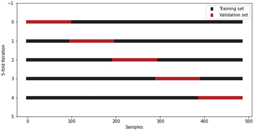
In total, 605 samples were randomly divided into a training set and a test set in a ratio of 0.8/0.2. The training set was used for the model establishment, while the test set was used to evaluate the model performance. There were six hyperparameters of XGBoost to be tuned by BO, including learning _rate, max_depth, min_child_weight, n_estimators, reg_alpha and gamma. The acquisition function selected in BO is the EI, the number of initial points is 5, the number of iterations for BO is set to 100. To acquire a better model generalization and reliability, 5-fold cross validation was implemented during model training to evaluate the combination of hyperparameters in each iteration of BO. As the results shown in Figure 6, the training set containing 484 samples was split into 5 folds, where the validation set in each iteration is marked with red block.

Figure 6. Separation results by 5-fold cross validation.

The BO-XGBoost model was established with the optimal combination of hyperparameters by BO. XGBoost has many hyperparameters that can be tuned for achieving good performance. Based on the application in previous studies, six important hyperparameters are chosen to be optimized in the current study, and the descriptions of the hyperparameters are as follows (Lv et al. 2020; Shi et al. 2021):

Learning_rate: The step size shrinkage reduces the influence of each individual tree and leaves space for future trees to improve the model. The smaller value will make the model more conservative.

Max_depth: The maximum depth of a tree. This hyperparameter controls the complexity of the tree models. Increasing this value will make the model more complex and easier to overfit, while a too small value will lead to the underfitting issue.

min_child_weight: The minimum sum of the instance weight (Hessian) needed in a child. At a leaf node, if the sum of instance weight is smaller than the value, the node will stop splitting and become a leaf. The larger value will make the model more conservative.

n_estimators: The maximum number of weak learners (i.e., CARTs). A too small value will result in the underfitting issue. In contrast, a too large value will significantly increase the computations, while the model will stop optimizing after the optimal value is reached.

reg_alpha: L1 regularization term on weights. The larger value will make the model more conservative.

gamma: Minimum loss reduction required to make a further split on a leaf node of the CART. The larger gamma will form the model more conservative.

A brief description and search space of each hyperparameter are shown in Table 4.

Table 4. Descriptions and search space of the hyperparameters optimized by BO (Lv et al. 2020; Shi et al. 2021).

Hyperparameter	Description	Search space of BO
learning _rate	Boosting learning rate	0.001 to 0.05
max_depth	The maximum depth of the tree model, to prevent overfitting	1 to 20
min_child_weight	The minimum sum of the weights in a child node, to prevent overfitting or underfitting	1 to 10
n_estimators	The number of base trees to fit	25 to 1000
reg_alpha	A regularization term	0.01 to 0.1
gamma	The minimum loss reduction required to split the tree	0.1 to 0.1

4.4. Results and analysis

4.4.1. The performance of BO on XGBoost

In the current study, BO aims to enhance the XGBoost by optimizing the process of hyperparameter tuning. As grid search (GS) is the most extensively used hyperparameter tuning method in literature, a comparison between the BO and GS was conducted to demonstrate the superiority of the BO in performance improvement on the original XGBoost. Four statistical metrics (i.e., $R^2$, RMSE, MAE, and adjusted $R^2$), running time and learning curves are used to evaluate the performance of BO and GS on XGBoost models.

The search space BO was implemented as presented in section 4.3. For GS, the same search space of each hyperparameter was set as: learning _rate ∈ {0.001, 0.01, 0.02, 0.05}, max_depth ∈ {1, 3 … 20}, min_child_weight ∈ {2, 4 … 10}, n_estimators ∈ {25, 75 … 1000}, reg_alpha ∈ {0.01, 0.05, 0.1} and gamma ∈ {0.1, 0.2, 0.3}. The 5-fold cross-validation was also used with GS. In total 36,000 candidates were achieved in each fold and 180,000 fits were obtained. Finally, although both BO and GS achieved their optimal combinations of hyperparameters, BO can find more precise values of each hyperparameters, as shown in Table 5.

Table 5. The optimal hyperparameter combinations determined by BO and GS.

	learning _rate	max_depth	min_child_weight	n_estimators	reg_alpha	gamma
BO	0.0484	3	1.3441	562	0.0314	0.2078
GS	0.05	3	2	76	0.1	0.3

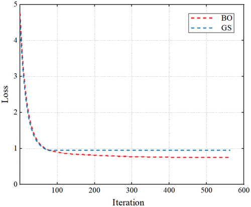
To evaluate the training process with the achieved hyperparameters, we plot the learning curves of BO and GS in the training set respectively. As can be seen from Figure 7, the loss of both BO and GS was relatively high at the beginning of training. Then, both BO and GS curves converged to their near minimum loss quickly within the first 50 iterations. The GS curve stopped descending after 76 iterations, while the loss of BO continued to decrease and eventually stabilized after 300 iterations. Finally, the loss of both BO and GS didn’t decrease anymore and stayed at relatively low value, indicating BO and GS have already provided their best optimization on XGBoost models. The learning curves show that BO achieved lower loss than GS after the optimization; consequently, BO could enhance the XGBoost with the higher model accuracy.

Figure 7. Learning curves of using BO and GS.

Then, the estimation performances and efficiency of BO-XGBoost and XGBoost are compared in Table 6, both of BO and GS achieved satisfactory estimation accuracy on the test set. BO-XGBoost achieved better outcomes for all four statistical metrics than the XGBoost tuned by GS, with higher $R^2$ ~0.9567 and adjusted $R^2$ ~0.9549, lower RMSE ~ 0.8690 and MAE ~ 0.4875 in test set. Meanwhile, BO took only 3.25 mins to optimize the XGBoost, while GS took 434.87 mins. Hence, the results show that BO increased the estimation accuracy of the XGBoost model and significantly boosted the training efficiency.

Table 6. Comparison between BO and GS on XGBoost.

Hyperparameters tuning method	Model performance evaluation metrics				Running time (min)
	$R^2$	RMSE	MAE	Adjusted $R^2$
BO	0.9567	0.8690	0.4875	0.9549	3.25
GS	0.9386	1.0349	0.5878	0.9348	434.87

4.4.2. Estimation performance comparison

The test set was used to validate the estimation performance of BO-XGBoost. As artificial neural network (ANN), support vector regression (SVR), multiple linear regression (MLR), and gradient boosting decision tree (GBDT) were the most frequently used methods in the relevant studies, these four benchmark models were implemented and investigated for comparison. The benchmark models used the same training set and test set with BO-XGBoost. The 5-fold cross-validation was also adopted in their training processes. To achieve their best performance on validation sets, BO-XGBoost and GBDT experienced 562 and 350 iterations respectively, while the BPNN had an epoch of 37. Table 7 shows that the BO-XGBoost provided the best estimation with $R^2$ ~0.9604, RMSE ~ 0.7705, MAE ~ 0.4309, and adjusted $R^2$ ~0.9588 in the training set; and $R^2$ ~0.9567, RMSE ~ 0.8690, MAE ~ 0.4875, and adjusted $R^2$ ~0.9549 in the validation set. Furthermore, BO-XGBoost had the smallest $R^2$ gap between the training set and validation set with a value of 0.0024, followed by GBDT, BPNN, SVM, and MLR with values of 0.0036, 0.0102, 0.0704, and 0.0385 respectively. This comparison indicates that the BO-XGBoost has good model performance and low risks of overfitting.

Table 7. 5-fold cross-validation results of training set and validation set.

	Model	Model performance
		$R^2$	RMSE	MAE	Adjusted $R^2$
Training set	BO-XGBoost	0.9604	0.7705	0.4309	0.9588
	GBDT	0.9421	0.9316	0.5344	0.9385
	BPNN	0.9105	1.1582	0.6630	0.9049
	SVM	0.8345	1.5749	0.6117	0.8242
	MLR	0.7013	2.1154	1.4042	0.6828
Validation set	BO-XGBoost	0.9580	0.8577	0.4560	0.9554
	GBDT	0.9385	1.0245	0.5888	0.9362
	BPNN	0.9003	1.2498	0.7046	0.8941
	SVM	0.7641	1.9757	0.9324	0.7494
	MLR	0.6628	2.3658	1.5975	0.6619

The performance of the BO-XGBoost and the benchmark models were assessed using the test set. For each model, the scatter points of the estimated cost versus actual cost are plotted with the regression fitting line in as shown in Figure 8. Due to data confidentiality, the cost of each sample was normalized into the range of [0,1] in the figure. According to the model performance shown in Table 8, the ensemble learning algorithms, XGBoost and GBDT, exhibited superiority to other ML algorithms with the higher $R^2$ values (over 0.9) and lower values of RMSE and MAE. BO-XGBoost provided the most satisfactory performance in the test set with $R^2$ ~0.9567, RMSE ~ 0.8690, MAE ~ 0.4875, and adjusted $R^2$ ~0.9549. Overall, the estimation accuracy of the models was ranked as: BO-XGBoost > GBDT > ANN > SVM > MLR.

Figure 8. Scatter plots with regression lines of test results among different models.

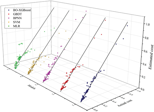
Table 8. Performance comparison of the different models on the test set.

Model	Model performance
	$R^2$	RMSE	MAE	Adjusted $R^2$
BO-XGBoost	0.9567	0.8690	0.4875	0.9549
GBDT	0.9376	1.0439	0.6109	0.9337
BPNN	0.8993	1.3252	0.7281	0.8930
SVM	0.7723	1.9934	0.8732	0.7582
MLR	0.6471	2.4813	1.6095	0.6253

4.4.3. Model interpretability

The relationships between the project features and the construction cost enable researchers to further investigate the important features and enhance their trust in the ML model. Therefore, SHAP is used to reveal how the features contribute to the construction cost.

The seven features’ importance was ranked from top to bottom in Figure 9. The horizontal axis and vertical axis represent the SHAP value and feature name, respectively, and each dot represents an electric substation sample. The color bar denotes the features’ values or encoded values, where blue denotes lower values and red denotes higher values. The most important feature that influences the construction cost was construction type, followed by voltage level, transformer capacity, N of transformers, substation type, location, and landform. Positive or negative SHAP values indicate that features increase or decrease the construction cost respectively. For construction type, the blue dots that denote new construction project contributes to a higher construction cost, while the red or purple dots that indicate main transformer or interval projects can contribute to lower construction cost. For the second and third important features, the high voltage level or transformer capacity often significantly increases the construction cost, while the low voltage level or transformer capacity has negative effects on the construction cost. The construction cost of electric substation will increase with more transformers being used.

Figure 9. SHAP explanation on the BO-XGBoost model.

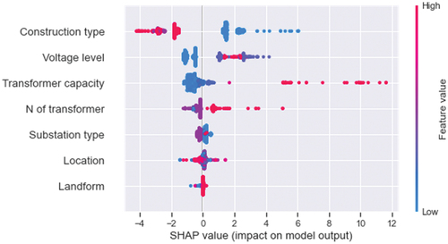
The results of SHAP suggest that project planners are more concerned about the top-ranked features such as construction type, voltage level, transformer capacity, and number of transformers in making the project plans.

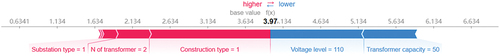
Moreover, we can use SHAP to investigate how each feature affects the construction cost in the individual project sample. As shown in Figure 10, the value of 3.97 in bold represents the estimated cost of the investigated sample, while the base value is the mean value of all the samples’ estimations. The color bar shows how the value of each project feature affects the estimation of the current sample, whereas the red and blue bars indicate the increasing and decreasing effects on the estimated cost, respectively. The length of the bar denotes the degree of the feature’s effect. In this sample, construction type, N of transformer, substation type, voltage level, and transformer capacity are the main cost drivers. Among the 5 features, the longest red bar of “Construction type = 1” has the most significant effect on this sample, which indicates “new construction project” is the most important reason to increase the cost of this substation. In contrast, the specifications of voltage level and transformer capacity have an influence on reducing the estimated cost toward the base value. Since the red bar is longer than the blue bar, the estimated cost of this substation is higher than the average cost of all the substation samples.

Figure 10. SHAP explanation on individual sample.

5. Discussion

5.1. Practical and theoretical implications

The proposed framework is expected to support the government or project planners in the challenging task of cost estimations in the conceptual phase of infrastructure projects.

Providing considerable cost estimation in the conceptual phase of projects is critical for making early decisions (Hyari, Al-Daraiseh, and El-Mashaleh 2016). Projects will experience various risks if they are implemented under unreliable cost estimation and inaccurate budget. In the current construction practice, cost estimations in the conceptual phase often rely on experts’ opinions and experience, which would lead to a large variance between the estimations and actual costs. The traditional cost estimation methods often require the quantities of construction materials and the corresponding cost of each unit following infrastructures’ design details (Akanbi and Zhang 2021). However, the design information can only be determined in the later stages of projects; consequently, those methods are hard to apply in the conceptual phase to support the early decision. In contrast, machine learning provides a different insight into conceptual cost estimation. ML is a data-driven method that makes the estimation by formulating the correlations between the projects’ features and the construction costs, without the requirements of detailed design information.

Based on the recent literature, there is a trend to use ensemble learning algorithms to solve conceptual cost estimations of infrastructures (Lee et al. 2022; Meharie et al. 2022). However, many of them mainly focused on evaluating the model accuracy in their test set, while overlooking that the infrastructure datasets are often relatively small. Existing studies also reported that the performance of some conventional machine learning methods or deep learning methods would decrease when dealing with low data volume (Hyari, Al-Daraiseh, and El-Mashaleh 2016). Therefore, XGBoost is selected in this study. In the case study results, the XGBoost is justified that can provide satisfactory performance on the conceptual cost estimation on electric substations even if the data set is relatively small. Compared with the benchmark models (including GBDT, BPNN, SVM, and MLR), XGBoost provided the highest estimation accuracy on training, validation, and test sets, and had the smallest performance gap between the training set and validation set with the lowest risk of overfitting.

Although previous studies have developed ML-based cost estimation models for different infrastructure projects, limited work was invested in improving the efficiency of developing their machine learning models. The traditional hyperparameter tuning method suffers from the inconsistency problem of accuracy-efficiency balance and could be very time-consuming to support early decision-making. Therefore, we adopted BO to bring Bayes’ rule into the training process of XGBoost, so that we can efficiently explore the near-optimal combination of the hyperparameters without traversing most of the poor combinations (Shin et al. 2020). Some studies have adopted BO in different fields, and found the superiority of BO over other hyperparameter tuning methods such as GS and random search (Shi et al. 2021). The results in our case study proved that BO can obviously increase the efficiency of XGBoost whilst improving the XGBoost estimation accuracy simultaneously. Since the model efficiency has to be considered in the realistic early decision-making of infrastructure projects, BO is the suitable hyperparameter optimization method to guarantee estimation accuracy with less time consumption in practice.

The feature is also a critical element in the machine learning modeling. Compared with the reviewed previous studies on conceptual cost estimation, this study puts more effort into the feature selection before ML model establishment and the feature analysis after providing estimations. During the feature selection, a widely used correlation analysis method was adopted to examine the correlations between each pair of the features. Furthermore, previous studies suggest that it is inadequate to only use correlation analysis, otherwise may still remain redundant features to mislead the model training (Guo et al. 2019). As the forward selection has been proven as a practical feature selection (FS) method based on regression (Mohsenijam, Siu, and Lu 2017), we added a forward selection method (based on XGBoost regression in this study) after the common process of correlation analysis, which aims to examine the real effect of each feature on improving or decreasing the estimation accuracy. The results identified that the selection of a feature named “N of transformer in the future” could reduce the estimation accuracy in different statistical metrics, consequently, this feature was removed. By combining the correlation analysis and FS, features with the predictive power for improving estimation accuracy could be selected for estimations.

In terms of feature analysis, SHAP is used to provide more information about how the features affect the costs of the projects to support the early decision by explaining the estimation results. Many of the previous studies on conceptual cost estimation paid little attention to the feature analysis after their estimations (Hyari, Al-Daraiseh, and El-Mashaleh 2016; Juszczyk 2020; Tijanic, Car-Pusic, and Sperac 2020), while some studies provided a simple feature importance ranking of their selected feature (Hashemi, Ebadati, and Kaur 2019; Lee et al. 2022; Meharie et al. 2022). However, in the conceptual phase, planners are concerned not only about the estimated cost of a project, but also about the main cost drivers and how they contribute to the estimated cost. Based on the understanding of the features’ effects on actual construction costs, the planners could adjust the project plan by changing one or more project’s features to satisfy both the financial budget and technical requirements. The current study provides both global and local explanations of the features’ contributions to the costs. As the individual substation sample in Section 4.4.3, the substation was estimated with a higher cost than the base value, which is most contributed by its construction type. If its estimated cost is unacceptable, the planner should abandon this new construction plan, and consider another kind of construction type such as a main transformer project instead.

In practice, the proposed framework can enhance decision-making in the early stage of infrastructure projects by integrating multi-step feature selection, XGBoost, BO, and SHAP. As the case study demonstrated, the framework can accurately estimate the construction cost of electric substations for different combinations of construction types, voltage levels, transformer capacities, number of transformers, substation types, locations, and landforms. This framework can provide accurate and efficient cost estimations, permitting the comparison of several project alternative plans to select the best project plan with the least cost to meet the technical requirement. For example, a project planner can quickly build an XGBoost model via BO, and then conduct the cost estimation to evaluate the effect of implementing different construction types and the effect of increasing the number of transformers on construction costs before making the practical decisions.

5.2. Applicability and generalizability

Based on Section 5.1, the applicability and generalizability of the proposed framework for different cases are further discussed in this section. Figure 11 demonstrates the generic application flow of the proposed framework on other cases of conceptual cost estimations and the advantages that can be generalized.

Figure 11. The applicability and generalizability of the proposed framework.

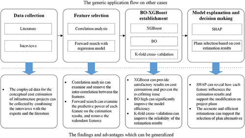
The BO-XGBoost framework has good applicability and generalizability for different cases, which can be reflected by the four stages in Figure 11 as follows:

When the proposed framework is employed for other cases, data collection should be implemented first since different kinds of infrastructures have their specific features. In the conceptual phase, few design information can be determined; consequently, the initial cost drivers are identified based on the literature and the opinions of experts. After that, the project data can be extracted from the public data sources, or the database from companies or departments.

Second, when dealing with different infrastructure datasets, feature selection is important to reduce the risk of the misleading caused by irrelevant features during model training and improve estimation accuracy. It is essential to select the valuable input features for when the datasets are relatively small (Huang, Li, and Xie 2015). Correlation analysis is a general method to examine and remove the inter-correlation between the features. However, a single use of correlation analysis is weak in evaluating the real influence of the features on the target variable (Guo et al. 2019). Therefore, forward search is used to examine the predictive power of each feature on the estimation results stepwise, and to retain the project features with predictive power and remove the redundant features more effectively in various infrastructure datasets.

Then, the BO-XGBoost model is developed by using the selected features. As mentioned in Section 2, the ML method has become a generic approach for the conceptual cost estimation of various infrastructures, which can formulate the relationships between the project features and the construction cost. XGBoost is an appropriate ML algorithm for conceptual cost estimations due to its high performance on estimation tasks and good ability of overfitting prevention (Dong et al. 2020). BO is applicable for many ML algorithms to optimize the hyperparameters efficiently, especially if many hyperparameters need to be optimized. BO can find the near-optimal hyperparameters in an efficient direction without evaluating most of the unsuitable hyperparameters combinations, while the time consumption of the traditional methods (i.e., GS) will increase exponentially to deal with a large number of hyperparameter candidates (Wu et al. 2019). The K-fold cross-validation is to split the training set of the dataset into k folds, and train the model for k times to validate the model performance in each iteration of BO, which can improve the reliability of the estimation results (Son, Kim, and Kim 2012).

Finally, this framework is not only to provide an estimated value of a project’s cost, but also to support the early decision-making based on the results of the estimations. Project plan alternatives can be compared and selected based on accurate and efficient cost estimations. When applying the proposed framework in other cases, SHAP can interpret the cost estimation results of ML models in terms of feature contributions. As demonstrated and discussed in Section 5.1, SHAP is used to explain how each feature influences the estimated costs at both the global level and individual project, which can help the project planner in the cost control and plan alternatives selection in the early stage. If the estimated cost is too high for an individual project, the planner can use SHAP to reveal the main contributing features, and change the features’ values under the technical requirement to reduce the project cost. The planner can also conduct the cost estimation to evaluate the effect of implementing different values of features on construction costs before selecting the project plan from the alternatives.

Furthermore, the applicability of the BO-XGBoost model is expressed by the high efficiency of model modification due to BO. The traditional hyperparameter tuning methods suffer from the inconsistency problem of accuracy-efficiency balance that can be very time-consuming (Wu et al. 2019). However, the issue of efficiency must be considered in the cost estimation for early decisions in practice. In response, BO is an efficient hyperparameter tuning method that can dramatically reduce the time consumption to find the optimal hyperparameter combination for XGBoost, and improve estimation accuracy. For example, in the case study of electric substations, the original XGBoost required approximately 133.8 times more time consumption (434.87 mins) than the BO-XGBoost (3.25 mins) for the model establishment and achieved lower estimation accuracy than BO. Moreover, infrastructure datasets often update due to the continuous collection of new project samples and changes in features for different estimation aims (e.g., installation cost and equipment cost), which can lead to the modification of the ML models. Since the time consumption of model modification can be significantly reduced via BO, it can also boost the efficiency of decision-making in the conceptual phase.

Therefore, the estimation model in the proposed framework can be easily expanded and modified to add more cost-related electric substation features in the future and more historical samples to train such a model. Based on the behavior of the methods discussed in Section 5.1 and Section 5.2, the scope of the proposed framework is flexible in adapting various cases of other infrastructures by using the corresponding project features and cost data with the proposed framework.

Furthermore, the BO-XGBoost can not only deal with the relatively small data set with overfitting prevention, but also has a strong ability to process large data sets. The outstanding performance of XGBoost on a large data set was evaluated when it was designed entirely in 2016 using a big database with 1.7 billion samples (Chen, Guestrin, and Assoc Comp 2016). In the construction industry, XGBoost has also been reliable when dealing with relatively large data sets. For example, XGBoost has been successfully used to predict the construction works’ post-accident disability status with a dataset of 47,938 samples (Koc, Ekmekcioglu, and Gurgun 2021). XGBoost is also desired to be effective when estimating the costs of mega projects, although there are only few existing studies on it. For example, Elmousalami (2020) compared 20 machine learning algorithms on the cost estimation of field canal improvement projects, and indicated XGBoost is the most satisfactory algorithm in their case study. Meharie et al. (2022). used the ensemble learning algorithm (with base learners of SVM and ANN) to estimate the construction cost of the power generation projects, while XGBoost is considered as a more state-of-the-art ensemble learning algorithm. Since the principle of XGBoost-based estimation remains the same, the estimation on mega projects also needs to collect a series of project features. However, since the mega project could be more complex than common infrastructure projects, more features are desired to be collected to describe and define the mega projects.

6. Conclusion

Estimating the conceptual cost of the infrastructure projects is an essential element in the project plan at the early stage and the success of the project implementation. In this study, a BO-XGBoost-based framework is proposed for the cost estimation of infrastructures in the conceptual phase. XGBoost is built as the estimator with its outstanding performance on various estimation problems and ability to handle relatively small infrastructure samples. Bayesian optimization (BO) enhances the XGBoost with higher estimation accuracy and significantly higher model efficiency. A multi-step feature selection method is designed to retain features with predictive power before model establishment by integrating correlation analysis, XGBoost, and forward search (FS). SHAP is used to explain the estimation results by revealing how the features contribute to the costs. A case study was demonstrated with 605 electric substation projects. The BO-XGBoost outperformed the benchmark models with satisfactory estimation accuracy of $R^2$ ~0.9567, adjusted $R^2$ ~0.9549, RMSE ~ 0.8690, and MAE ~ 0.4875. BO not only improves the estimation accuracy of XGBoost, but also significantly reduces the model establishment time from 434.87 mins to 3.25 mins. In addition, SHAP is used to interpret the estimation results by revealing how the features contribute to the project cost, which brings more information for supporting early decision-making in practice. The innovation of the proposed framework is to provide more accurate, efficient, and explainable cost estimations in the conceptual phase of infrastructure projects by integrating the multi-step feature selection, XGBoost, BO, and SHAP. Furthermore, the framework can assist the government and project planners make reliable investment management and acceptable project plans.

This study is not free from limitations. Since the features are selected via a data-driven method, the results of selection can be adjusted according to experts’ opinions for different situations or databases in practice. Second, although the BO-XGBoost performs well in the case study, collecting more electric substation samples could further enhance the reliability of the estimating models.

Future works could focus on using the proposed framework in more kinds of infrastructure projects (such as bridges and power plants) and investigate the estimation results. Second, project data management (including data record, classification, and storage) could be enhanced toward more accurate cost estimations. If the projects are described with more detailed information in the conceptual phase, more cost-related features with predictive power could be explored for cost estimations during the feature selection process. Furthermore, as AI technology grows, the proposed framework can be further developed with more advanced machine learning algorithms.

Acknowledgements

The authors would like to appreciate the related companies which accepted our survey and data support. The authors also would like to appreciate Dr. Shenghua Zhou in Southeast University for his valuable suggestions on writing, and Wenfei Lu in Southeast University for his support.

Disclosure statement

No potential conflict of interest was reported by the author(s).

Additional information

Notes on contributors

Jiashu Zhang

Jiashu Zhang is a PhD candidate in the Department of Construction and Real Estate, School of Civil Engineering, Southeast University. He also has a multidisciplinary background in electrical and electronic engineering. His main research interests include project management, machine learning, and low-carbon city management.

Jingfeng Yuan

Jingfeng Yuan is a professor in the Department of Construction and Real Estate, School of Civil Engineering, Southeast University. Dr. Yuan received his PhD in Southeast University. His main research direction is project management, intelligent construction, and big data analytics.

Amin Mahmoudi

Amin Mahmoudi is a researcher at the Southeast University, Nanjing, China. He was selected as the World’s Top 2% Scientists by Stanford University. He published nearly 55 papers in top-tier journals, including Information Sciences, Resources Policy, Expert Systems with Applications, Business Strategy and the Environment, IEEE Transactions on Engineering Management, etc. He developed a method titled Ordinal Priority Approach (OPA) for intelligent decision-making, which was used widely by scholars in various fields of study. He also developed web-based software titled “OPA Solver” that can be employed for decision-making in academia and industry. He is an editor in SN Operations Research Forum, The Journal of Grey System, Modern Supply Chain Research & Applications, Journal of Project Management, and Management Science Letters. He also published two books in the field of project management in 2013 and 2016. His main research interest is project management, supply chain management, decision science, and data analysis.

Wenying Ji

Wenying Ji is an assistant professor in the Department of Civil, Environmental & Infrastructure Engineering, George Mason University. Dr. Ji received his PhD in Construction Engineering and Management from the University of Alberta. Dr. Ji is an interdisciplinary scholar focused on the integration of advanced data analytics and complex system modeling to enhance the overall performance of infrastructure systems. His e-mail address is [email protected].

Qiushi Fang

Qiushi Fang obtained his master degree in the Department of Electrical and Electronic Engineering, The University of Manchester. His main research direction is machine learning and digital signal processing.

References

- AACE, AACE International recommended practices. 2004.
- Ahn, J., S. H. Ji, S. J. Ahn, M. Park, H. S. Lee, N. Kwon, E. B. Lee, and Y. Kim. 2020. “Performance Evaluation of Normalization-Based CBR Models for Improving Construction Cost Estimation.” Automation in Construction 119. https://doi.org/10.1016/j.autcon.2020.103329.
- Akanbi, T., and J. S. Zhang. 2021. “Design Information Extraction from Construction Specifications to Support Cost Estimation.” Automation in Construction 131. https://doi.org/10.1016/j.autcon.2021.103835.
- Almasabha, G., K. F. Al-Shboul, A. Shehadeh, and O. Alshboul. 2023. ”Machine learning-based models for predicting the shear strength of synthetic fiber reinforced concrete beams without stirrups.“ Structures 52. https://doi.org/10.1016/j.istruc.2023.03.170.
- Alshboul, O., A. Shehadeh, G. Almasabha, R. E. A. Mamlook, and A. S. Almuflih. 2022. “Evaluating the Impact of External Support on Green Building Construction Cost: A Hybrid Mathematical and Machine Learning Prediction Approach.” Buildings 12 (8): 1256. https://doi.org/10.3390/buildings12081256.
- Antwarg, L., R. M. Miller, B. Shapira, and L. Rokach. 2021. “Explaining Anomalies Detected by Autoencoders Using Shapley Additive Explanations.” Expert Systems with Applications 186:115736. https://doi.org/10.1016/j.eswa.2021.115736.
- Bai, B., J. Y. Zhang, X. Wu, G. W. Zhu, and X. Y. Li. 2021. “Reliability Prediction-Based Improved Dynamic Weight Particle Swarm Optimization and Back Propagation Neural Network in Engineering Systems.” Expert Systems with Applications 177. https://doi.org/10.1016/j.eswa.2021.114952.
- Beniwal, M., A. Singh, and N. Kumar. 2023. “Forecasting Long-Term Stock Prices of Global Indices: A Forward-Validating Genetic Algorithm Optimization Approach for Support Vector Regression.” Applied Soft Computing 145:110566. https://doi.org/10.1016/j.asoc.2023.110566.
- Bhargava, A., S. Labi, S. K. Chen, T. U. Saeed, and K. C. Sinha. 2017. “Predicting Cost Escalation Pathways and Deviation Severities of Infrastructure Projects Using Risk-Based Econometric Models and Monte Carlo Simulation.” Computer-Aided Civil and Infrastructure Engineering 32 (8): 620–640. https://doi.org/10.1111/mice.12279.
- Cao, Y., B. Ashuri, and M. Baek. 2018. “Prediction of Unit Price Bids of Resurfacing Highway Projects Through Ensemble Machine Learning.” Journal of Computing in Civil Engineering 32 (5). https://doi.org/10.1061/(ASCE)CP.1943-5487.0000788.
- Chakraborty, D., H. Elhegazy, H. Elzarka, and L. Gutierrez. 2020. “A Novel Construction Cost Prediction Model Using Hybrid Natural and Light Gradient Boosting.” Advanced Engineering Informatics 46:101201. https://doi.org/10.1016/j.aei.2020.101201.
- Chen, T. Q., C. Guestrin, and M. Assoc Comp. 2016. “XGBoost: A Scalable Tree Boosting System.” In 22nd ACM SIGKDD International Conference on Knowledge Discovery and Data Mining (KDD), 785–794. San Francisco, CA.
- Diekmann, J. E. 1983. “Probabilistic Estimating: Mathematics and Applications.” Journal of Construction Engineering and Management 109 (3): 297–308. https://doi.org/10.1061/(ASCE)0733-9364(1983)109:3(297).
- Dong, W., Y. M. Huang, B. Lehane, and G. W. Ma. 2020. “XGBoost Algorithm-Based Prediction of Concrete Electrical Resistivity for Structural Health Monitoring.” Automation in Construction 114. https://doi.org/10.1016/j.autcon.2020.103155.
- Dursun, O., and C. Stoy. 2016. “Conceptual Estimation of Construction Costs Using the Multistep Ahead Approach.” Journal of Construction Engineering and Management 142 (9). https://doi.org/10.1061/(ASCE)CO.1943-7862.0001150.
- Elmousalami, H. H. 2020. “Artificial Intelligence and Parametric Construction Cost Estimate Modeling: State-Of-The-Art Review.” Journal of Construction Engineering and Management 146 (1). https://doi.org/10.1061/(ASCE)CO.1943-7862.0001678.
- ElMousalami, H. H., A. H. Elyamany, and A. H. Ibrahim. 2018. “Predicting Conceptual Cost for Field Canal Improvement Projects.” Journal of Construction Engineering and Management 144 (11). https://doi.org/10.1061/(ASCE)CO.1943-7862.0001561.
- Gu, Q. H., Y. X. Chang, N. X. Xiong, and L. Chen. 2021. “Forecasting Nickel Futures Price Based on the Empirical Wavelet Transform and Gradient Boosting Decision Trees.” Applied Soft Computing 109. https://doi.org/10.1016/j.asoc.2021.107472.
- Guo, J. Q., L. Yang, R. F. Bie, J. G. Yu, Y. Gao, Y. Shen, and A. Kos. 2019. “An XGBoost-Based Physical Fitness Evaluation Model Using Advanced Feature Selection and Bayesian Hyper-Parameter Optimization for Wearable Running Monitoring.” Computer Networks 151:166–180. https://doi.org/10.1016/j.comnet.2019.01.026.
- Hashemi, S. T., E. O. M. Ebadati, and H. Kaur. 2019. “A Hybrid Conceptual Cost Estimating Model Using ANN and GA for Power Plant Projects.” Neural Computing & Applications 31 (7): 2143–2154. https://doi.org/10.1007/s00521-017-3175-5.
- He, X., R. Liu, and C. J. Anumba. 2021. “Data-Driven Insights on the Knowledge Gaps of Conceptual Cost Estimation Modeling.” Journal of Construction Engineering and Management 147 (2). https://doi.org/10.1061/(ASCE)CO.1943-7862.0001963.
- Huang, J. L., Y. F. Li, and M. Xie. 2015. “An Empirical Analysis of Data Preprocessing for Machine Learning-Based Software Cost Estimation.” Information and Software Technology 67:108–127. https://doi.org/10.1016/j.infsof.2015.07.004.
- Huang, Y. F., and S. W. Meng. 2019. “Automobile Insurance Classification Ratemaking Based on Telematics Driving Data.” Decision Support Systems 127. https://doi.org/10.1016/j.dss.2019.113156.
- Hyari, K. H., A. Al-Daraiseh, and M. El-Mashaleh. 2016. “Conceptual Cost Estimation Model for Engineering Services in Public Construction Projects.” Journal of Management in Engineering 32 (1). https://doi.org/10.1061/(ASCE)ME.1943-5479.0000381.
- IM Almadi, A., R. E. Al Mamlook, I. Ullah, O. Alshboul, N. Bandara, and A. Shehadeh. 2022. “Vehicle Collisions Analysis on Highways Based on Multi-User Driving Simulator and Multinomial Logistic Regression Model on US Highways in Michigan.” International Journal of Crashworthiness 28 (6): 770–785. https://doi.org/10.1080/13588265.2022.2130608.
- Juszczyk, M. 2020. “On the Search of Models for Early Cost Estimates of Bridges: An SVM-Based Approach.” Buildings 10 (1): 2. https://doi.org/10.3390/buildings10010002.
- Karaca, I., D. D. Gransberg, and H. D. Jeong. 2020. “Improving the Accuracy of Early Cost Estimates on Transportation Infrastructure Projects.” Journal of Management in Engineering 36 (5). https://doi.org/10.1061/(ASCE)ME.1943-5479.0000819.
- Kim, D., K. Kwon, K. Pham, J. Y. Oh, and H. Choi. 2022. “Surface Settlement Prediction for Urban Tunneling Using Machine Learning Algorithms with Bayesian Optimization.” Automation in Construction 140:104331. https://doi.org/10.1016/j.autcon.2022.104331.
- Koc, K., O. Ekmekcioglu, and A. P. Gurgun. 2021. “Integrating Feature Engineering, Genetic Algorithm and Tree-Based Machine Learning Methods to Predict the Post-Accident Disability Status of Construction Workers.” Automation in Construction 131:103896. https://doi.org/10.1016/j.autcon.2021.103896.
- Lee, J. G., H. S. Lee, M. Park, and J. Seo. 2022. “Early-stage cost estimation model for power generation project with limited historical data.” Engineering, Construction & Architectural Management 29 (7): 2599–2614. https://doi.org/10.1108/ECAM-04-2020-0261.
- Lim, S., and S. Chi. 2019. “Xgboost application on bridge management systems for proactive damage estimation.” Advanced Engineering Informatics 41. https://doi.org/10.1016/j.aei.2019.100922.
- Liu, Y. M., L. Liu, L. Yang, L. Hao, and Y. Bao. 2021. “Measuring Distance Using Ultra-Wideband Radio Technology Enhanced by Extreme Gradient Boosting Decision Tree (XGBoost).” Automation in Construction 126:103678. https://doi.org/10.1016/j.autcon.2021.103678.
- Lundberg, S. and S. I. Lee. A Unified Approach to Interpreting Model Predictions. in Nips. 2017.
- Luong, P., D. Nguyen, S. Gupta, S. Rana, and S. Venkatesh. 2021. “Adaptive Cost-Aware Bayesian Optimization.” Knowledge-Based Systems 232:107481. https://doi.org/10.1016/j.knosys.2021.107481.
- Lv, F., J. J. Wang, B. Cui, J. Yu, J. E. Sun, and J. Zhang. 2020. “An Improved Extreme Gradient Boosting Approach to Vehicle Speed Prediction for Construction Simulation of Earthwork.” Automation in Construction 119:103351. https://doi.org/10.1016/j.autcon.2020.103351.
- Mahmoodzadeh, A., H. R. Nejati, and M. Mohammadi. 2022. “Optimized Machine Learning Modelling for Predicting the Construction Cost and Duration of Tunnelling Projects.” Automation in Construction 139. https://doi.org/10.1016/j.autcon.2022.104305.
- Meharie, M. G., W. J. Mengesha, Z. A. Gariy, and R. N. N. Mutuku. 2022. “Application of Stacking Ensemble Machine Learning Algorithm in Predicting the Cost of Highway Construction Projects.” Engineering, Construction & Architectural Management 29 (7): 2836–2853. https://doi.org/10.1108/ECAM-02-2020-0128.
- Mohsenijam, A., M. F. F. Siu, and M. Lu. 2017. “Modified Stepwise Regression Approach to Streamlining Predictive Analytics for Construction Engineering Applications.” Journal of Computing in Civil Engineering 31 (3). https://doi.org/10.1061/(ASCE)CP.1943-5487.0000636.
- Rao, H., X. Shi, A. K. Rodrigue, J. Feng, Y. Xia, M. Elhoseny, X. Yuan, and L. Gu. 2019. “Feature Selection Based on Artificial Bee Colony and Gradient Boosting Decision Tree.” Applied Soft Computing 74:634–642. https://doi.org/10.1016/j.asoc.2018.10.036.
- Rodriguez-Calvo, A., P. Frias, J. Reneses, R. Cossent, and C. Mateo. 2014. “Optimal Investment in Smart MV/LV Substations to Improve Continuity of Supply.” International Journal of Electrical Power & Energy Systems 62:410–418. https://doi.org/10.1016/j.ijepes.2014.04.062.
- Shahriari, B., K. Swersky, Z. Y. Wang, R. P. Adams, and N. de Freitas. 2016. “Taking the Human Out of the Loop: A Review of Bayesian Optimization.” Proceedings of the IEEE 104 (1): 148–175. https://doi.org/10.1109/JPROC.2015.2494218.
- Shehadeh, A., O. Alshboul, R. E. Al Mamlook, and O. Hamedat. 2021. “Machine Learning Models for Predicting the Residual Value of Heavy Construction Equipment: An Evaluation of Modified Decision Tree, LightGbm, and XGBoost Regression.” Automation in Construction 129. https://doi.org/10.1016/j.autcon.2021.103827.
- Shin, S., Y. Lee, M. Kim, J. Park, S. Lee, and K. Min. 2020. “Deep Neural Network Model with Bayesian Hyperparameter Optimization for Prediction of NOx at Transient Conditions in a Diesel Engine.” Engineering Applications of Artificial Intelligence 94. https://doi.org/10.1016/j.engappai.2020.103761.
- Shi, R., X. Y. Xu, J. M. Li, and Y. Q. Li. 2021. “Prediction and Analysis of Train Arrival Delay Based on XGBoost and Bayesian Optimization.” Applied Soft Computing 109. https://doi.org/10.1016/j.asoc.2021.107538.
- Son, H., C. Kim, and C. Kim. 2012. “Hybrid Principal Component Analysis and Support Vector Machine Model for Predicting the Cost Performance of Commercial Building Projects Using Pre-Project Planning Variables.” Automation in Construction 27:60–66. https://doi.org/10.1016/j.autcon.2012.05.013.
- Sovacool, B. K., A. Gilbert, and D. Nugent. 2014. “An International Comparative Assessment of Construction Cost Overruns for Electricity Infrastructure.” Energy Research & Social Science 3:152–160. https://doi.org/10.1016/j.erss.2014.07.016.
- Tayefeh Hashemi, S., O. M. Ebadati, and H. Kaur. 2020. “Cost Estimation and Prediction in Construction Projects: A Systematic Review on Machine Learning Techniques.” SN Applied Sciences 2 (10). https://doi.org/10.1007/s42452-020-03497-1.
- Tijanic, K., D. Car-Pusic, and M. Sperac. 2020. “Cost estimation in road construction using artificial neural network.” Neural Computing & Applications 32 (13): 9343–9355. https://doi.org/10.1007/s00521-019-04443-y.
- Vasconcelos, T. D., D. de Souza, G. C. D. Virgolino, C. L. C. Mattos, and J. P. P. Gomes. 2022. “Self-Tuning Portfolio-Based Bayesian Optimization.” Expert Systems with Applications 188:115847. https://doi.org/10.1016/j.eswa.2021.115847.
- Wang, R., V. Asghari, C. M. Cheung, S. C. Hsu, and C. J. Lee. 2022. “Assessing Effects of Economic Factors on Construction Cost Estimation Using Deep Neural Networks.” Automation in Construction 134. https://doi.org/10.1016/j.autcon.2021.104080.
- Wang, J. H., Y. T. Ren, T. H. Shu, L. Y. Shen, X. Liao, N. Yang, and H. M. He. 2020. “Economic Perspective-Based Analysis on Urban Infrastructures Carrying Capacity — a China Study.” Environmental Impact Assessment Review 83:83. https://doi.org/10.1016/j.eiar.2020.106381.
- Wu, J., X. Y. Chen, H. Zhang, L. D. Xiong, H. Lei, and S. H. Deng. 2019. “Hyperparameter Optimization for Machine Learning Models Based on Bayesian Optimization.” Journal of Electronic Science and Technology 17 (1): 26–40.
- Xue, P. N., Y. Jiang, Z. G. Zhou, X. Chen, X. M. Fang, and J. Liu. 2019. “Multi-Step Ahead Forecasting of Heat Load in District Heating Systems Using Machine Learning Algorithms.” Energy 188:116085. https://doi.org/10.1016/j.energy.2019.116085.
- Xu, X. M., L. Y. Peng, Z. S. Ji, S. P. Zheng, Z. X. Tian, and S. P. Geng. 2021. “Research on Substation Project Cost Prediction Based on Sparrow Search Algorithm Optimized BP Neural Network.” Sustainability 13 (24).
- Yun, K. K., S. W. Yoon, and D. Won. 2021. “Prediction of Stock Price Direction Using a Hybrid GA-XGBoost Algorithm with a Three-Stage Feature Engineering Process.” Expert Systems with Applications 186:115716. https://doi.org/10.1016/j.eswa.2021.115716.
- Zhang, C. X., and J. B. Fan. 2018. “Chapter 5 - UHVAC Substation and Main Electrical Equipment.” In UHV Transmission Technology, edited by T. C. E. P. R. Institute, 165–236, China: Academic Press.
- Zhang, H. B., D. D. Qiu, R. Z. Wu, Y. X. Deng, D. H. Ji, and T. Li. 2019. “Novel Framework for Image Attribute Annotation with Gene Selection XGBoost Algorithm and Relative Attribute Model.” Applied Soft Computing 80:57–79. https://doi.org/10.1016/j.asoc.2019.03.017.
- Zhou, H., S. Huang, P. Zhang, B. Ma, P. Ma, and X. Feng. 2023. “Prediction of Jacking Force Using PSO-BPNN and PSO-SVR Algorithm in Curved Pipe Roof.” Tunnelling and Underground Space Technology138:105159. https://doi.org/10.1016/j.tust.2023.105159.