ANN prediction model of final construction cost at an early stage

ABSTRACT

Previous studies developed models to predict final construction cost (FCC) values based on many inputs, which makes them difficult to use. However, relying on models with relatively few inputs will reduce the accuracy of the prediction results. This paper aims to develop an artificial neural network (ANN) model to predict the FCC based on contract cost (CC), contract duration, and project sector at an early stage of a project. The data collected and used for the ANN model was 135 Saudi Arabian construction projects. The Zavadskas and Turskis logarithmic approaches, and the Pasini method were utilized to overcome the limited data. Then, the ANN model was developed through two stages. The purpose of the first stage was to enhance the data by identifying the abnormal data using absolute percentage errors (APE). The enhanced data was used to develop the ANN in the second stage. The finding showed that the ANN model provided an average MAPE (mean absolute percentage error) of 18.7%. The MAPE of the ANN model is decreased to 8.7% on average by deleting data with an APE higher than 35%. The model allows stakeholders to evaluate the financial importance of potential risks and develop appropriate risk management strategies.

KEYWORDS:

• Forecast
• cost
• neural network
• MAPE
• sector
• determination
• contract
• duration

1. Introduction

Saudi Arabia is the largest construction market in the region, and studies have indicated that it is one of the ten countries with 73% of investment in construction and infrastructure in the world (AlMunif and Almutairi, 2021). With this vast and growing investment in the construction sector comes the importance of promoting and increasing awareness about the value of adopting modern and advanced technologies and methods in engineering and managing construction projects to obtain reliable and sustainable outputs. Managing the project’s costs is the most significant aspect of executing construction projects. Costs are considered primary criteria in the projects’ feasibility studies and decision-making at the early stages of the project (Heralova 2017). Furthermore, time and costs are the main factors that shall be considered throughout the project implementation phases, starting from cost estimation and planning through project performance measurement and control until the completion of the project (Olawale and Sun 2010). The data relating to the project’s costs is critical for an informed decision-making process and to indicate any deviation from the correct implementation of the project’s desired goals. Thus, a construction project’s success depends on accurate assessment and forecasting of the project budget, where cost overruns are serious issues hindering the appropriate execution of construction projects.

Several studies have indicated the critical issue of the construction industry with time and cost overruns. The overall aim of these studies is attributed to the need for more accuracy in the project cost estimate and budget allocations (Algahtany, Alhammadi, and Kashiwagi 2016). Alzara, Kashiwagi, and Al-Tassan (2018) analyzed time and cost overruns in the construction projects of a higher education institute. They found that bids submitted by the contractors eventually awarded the contract were much lower than the market project costs.

Employing advanced techniques and methods with high accuracies, such as artificial neural networks and regression analysis, to predict costs at project completion (final construction cost) will improve the planning and control processes. Moreover, this will be reflected in the projects’ performance in the construction industry. The results of assessments and studies that adopted predictive analytic techniques indicated that these techniques had proven their ability to give high-accuracy predictive results. Predictive analytics can be defined as the systematic analysis of data to elaborate models for prediction using computational techniques (Castro Miranda et al. 2022). The primary function of predictive modeling is to predict future observations using data-mining algorithms or statistical model data (Ngo et al., 2020).

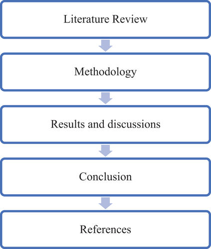
Most studies focus on building types of construction projects, so a need exists to widely apply time and cost models for different construction projects (Elmousalami 2020). Moreover, the model trained in different geographic zones with different legislations and regulations may perform differently in Saudi Arabia. The cost modeling research area needs more studies to develop intelligent models to interpret the resulting time and cost forecasting and analyze the input model’s parameters (Elmousalami 2020). Based on the literature review, regression analysis methods and artificial neural networks have shown promising results in predicting the final construction cost of construction projects with forecasting accuracy that outperforms traditional methods. On the other hand, machine learning techniques are complex, require significant historical data, and take a long time to complete. As a result, the ANN method cannot be used with relatively small data. In order to close the gap, the 135 data of Saud Arabia construction projects were first normalized by Zavadskas and Turskis logarithmic standardized and maximized using the method introduced by (Pasini 2015). The 135 data were separated into ten subgroups, one of which was designated testing data and was not considered by the ANN model. The nine data categories were created using the order testing data. The ANN model uses each data group, representing 90% of the total data, exclusively as training data, with the testing data set to zero. The nine ANN models were run multiple times to monitor relative error and prevent overfitting errors. Each data set represents 90% of the total data and is used fully as training data for the ANN model, with the testing data set to zero. The nine ANN models were repeatedly run. The absolute percentage error (APE) was then calculated based on the observed FCC, and the FCC was computed using the ANN model. The APEs were calculated throughout the training data. For each training group, the data were enhanced by removing abnormal data with a high residual error, which produced the modified training data. Based on the modified training data, the ANN theory was established. The paper’s contribution is to develop an ANN model for predicting the FCC of a project at an early stage based on three common input variables. However, the main challenge of the developed model was the limited available data used to train and test the ANN model. The components of the paper are shown in Figure 1.

Figure 1. Research methodology.

2. Literature review

Project cost accurate estimation is a decisive factor in its success, as cost estimation begins at the design stage. Issues of miscalculation appear at the bidding stage (the difference in the owner’s cost estimation from the lowest bid) and the construction project stage (the difference in the cost at the project completion from the contract cost at the beginning of the implementation project). Many studies discussed the miscalculation of the cost in the pre-bid contract in terms of studying the factors causing the miscalculation (Alsugair 2022; Baek et al. 2019; Flyvbjerg, Holm, and Buhl 2002; Li, Zheng, and Ashuri 2022; Mahamid 2018; Saqer et al. 2020) or developing a model for estimating the value of the contract (Badawy 2020; Lowe 2006; Natarajan 2022, Wu and Xu 2013; Ye 2021). Studies that reviewed and assessed the cost difference generated during project execution were divided into two groups: cost related to contractor and cost related to client/or owner (final contract cost). This paper focuses on developing the FCC. Therefore, the review of developing predictive models to estimate the FCC at an early was displayed in the following literature survey section.

Many factors affect construction project costs, and some present significant challenges in the cost forecasting process. The reliability of the prediction approach determines whether the prediction models are successful or unsuccessful (Moghayedi and Windapo 2021). Relying on variables with little relationship to the project cost to forecast cost will increase the amount of calculation and reduce the accuracy of the forecasting outcomes (Elmousalami 2020). Various techniques and methods are available to develop predictive models of the relationships among various variables in the construction industry, such as regression analysis methods, time series analysis, and machine learning techniques.

Regression is a technique to predict the target variable’s numerical value based on input variables, while classification automatically emulates decisions through trained data sets (Bilal et al. 2016). Common variations of regression include simple linear regression, multiple linear regression, and logistic regression. Prominent classification algorithms include decision trees, Naïve Bayes, neural networks, K-nearest neighbor, support vector machines, random forests, time series forecasting, and partial least squares (Bilal et al. 2016). Alcineide et al. (2021) utilized a cost forecasting model based on artificial intelligence techniques, specifically on artificial neural networks. In addition, Elhegazy, Chakraborty et al. (2022) utilized artificial intelligence to predict the cost of composite floors for buildings. The neural model utilized in the cost estimate completed a learning process that generated an average percentage inaccuracy between 5 and 9% when applied to new data.

Machine learning algorithms are developed to recognize patterns and relationships within datasets and use them to make predictions or take actions. Several studies utilize ML in different applications, such as the prediction of residual value of heavy equipment (Shehadeh et al. 2021), computing shear strength of reinforced slender beams without stirrup (Alshboul, Almasabha et al. 2022), establishing potential liquidated damages associated with project delays (Alshboul, Shehadeh et al. 2022), estimating synthetic fiber-reinforced concrete beams’ shear strength without stirrups (Almasabha et al. 2023), and assessing the efficiency and output of the steel structural project (Elhegazy, Badra et al. 2022).

Elmousalami (2020) has reviewed different computational intelligence techniques and methods to develop practical prediction models. The study focuses on reviewing the most common artificial intelligence (AI) techniques for cost modeling, such as fuzzy logic (FL) models, artificial neural networks (ANNs), case-based reasoning (CBR), diction tree (DT), random forest (RF), supportive vector machine (SVM), adaptive boosting (AdaBoost), scalable boosting trees, extreme gradient boosting (XGBoost). In addition, Chakraborty et al. (2020) conducted a comparative analysis of the predictive powers of six distinct machine learning algorithms: random forest, extreme gradient boosting, light gradient boosting, natural gradient boosting, artificial neural network, and linear regression using extensive data (4477 data points) to estimate construction cost. However, this method required extensive data to create a model.

FL creates fuzzy rules to represent the expertise of the experts. In fuzzy systems, it is represented by membership functions, which range from zero to one. The shape of MF largely influences the effectiveness of a fuzzy model. A set of operations on fuzzy sets can be carried out once these functions have been determined for each dependent and independent parameter. These operations include the -cut of a fuzzy set, the complement of a fuzzy set, the intersection of fuzzy sets, and the union of fuzzy sets. When linguistic concepts cannot be represented as quantitative terms, they are employed to represent the system properties (Zadeh 1976). On the other hand, it may be challenging to interpret fuzzy logic models physically. The linguistic rules and fuzzy membership functions used in the model may not directly correspond to the underlying physical phenomena of the FCC process. This lack of physical interpretability can make gaining insights into the actual mechanisms and relationships governing the process difficult.

The SVM algorithm is a well-liked machine learning algorithm that can handle high-dimensional data and complex decision limits. SVM is a supervised machine-learning technique that can solve classification and regression issues (Vapnik 2006). By maximizing the margin and the distance between the hyperplanes, the goal is to reduce the number of incidents of misclassification. SVMs, however, may be computationally expensive, mainly when working with massive datasets or high-dimensional feature spaces. With an increase in the number of training instances and the dimensionality of the data, SVMs need more memory and training time. Therefore, SVM training on large datasets can be time-consuming and demand a lot of computer power (Osuna and Girosi 1998).

DT is a supervised machine learning model that uses a repeating splitting method to separate the input data into hierarchical rules on each tree node. The relevance of data attributes can be determined using DT’s generated logic statements and interpretable rules (Perner, Zscherpel, and Jacobsen 2001). Due to its splitting process, DT can avoid the dimensionality curse while offering high-performance processing efficiency (Prasad, Iverson, and Liaw 2006). However, DT performs when dealing with time series, noisy, or nonlinear data (Curram and Mingers 1994). Additionally, as DT is known to have high variation, they may be sensitive to even little modifications in the training data. Distinct splits or modifications in the training data might produce noticeably distinct tree architectures and, as a result, diverse predictions (Dietterich and Kong 1995).

According to (Breiman 2001), RF is a bagging ensemble learning model that can produce precise performance without experiencing overfitting problems. In order to create a forest of trees based on random feature subsets, RF algorithms create bootstrap samples. However, RF is unable to decipher the generated forecasts. On the other hand, RF can get complicated, mainly when working with high-dimensional data or many trees. Interpreting the specific contributions of each tree and comprehending the underlying decision-making process becomes more difficult as the number of trees rises. In areas where model explainability and transparency are essential, the lack of interpretability may be a drawback (Aria, Cuccurullo, and Gnasso 2021).

AdaBoost is an algorithm that improves the performance of soft learning algorithms. It is also known as adaptive resampling (Schapire 1990). AdaBoost is one of many boosting algorithms, although it is vulnerable to noisy and outlier data sets. Outliers significantly impact the model’s learning process, which can result in overfitting or poor generalization. If the dataset has a lot of noise or outliers, the boosting method could need assistance to make accurate predictions (Cheki, Jazayeri-Rad, and Karimi 2016).

XGBoost is a large-scale machine learning system that can construct a highly scalable end-to-end ensemble tree-boosting system. According to (Chen and Guestrin 2016), XGBoost uses parallel computing to lower computational complexity and accelerate learning efficiently. For optimum performance, XGBoost requires careful tuning of several hyperparameters. Finding the ideal selection of parameters can be time-consuming and difficult, particularly for complicated datasets. Subpar results or overfitting may occur from insufficient parameter adjustment (Qin et al. 2021).

CBR is a cycle in which prior cases are studied to solve current cases. The four basic CBR procedures are retrieving, reusing, amending, and retaining. The retrieving procedure resolves a new case by retrieving the data from earlier cases. Key characteristics might be used to characterize the case. Retaining involves adding the new case to the existing case base to update the previously stored former cases (Aamodt and Plaza 1994). It can be challenging to locate pertinent instances in the case library and determine how closely they resemble the current issue. The caliber and representativeness of the examples in the library have a significant impact on CBR’s efficacy. Inaccurate or inadequate solutions may result from a case library that is deficient in information, outdated, or lacks diversity (Marín-Veites and Bach 2022).

Elmousalami (2020) summarized that the results of 20 AI techniques showed that the most accurate and suitable method is XGBoost with 9.091% and 0.929 based on mean absolute percentage error (MAPE) and adjusted R², respectively.

Moghayedi and Windapo (2021) compared the Adaptive Neuro-Fuzzy Inference System (ANFIS), a machine learning technique, to Stepwise Regression Analysis (SRA), a classical statistical method, in the prediction of the size of the impact of uncertainty events on the construction cost of highway projects. The study concluded that using intelligent methods such as ANFIS will minimize the potential inconsistency of correlations in construction cost and cost prediction. However, regression analysis methods are relatively easy to implement. The method is simple for determining how the independent and dependent variables relate.

Bayram, Bayram and Al-Jibouri (2016) investigated the adequacy of the five nontraditional approaches. The approaches are multilayer perceptron (MLP), radial basis function (RBF), grid partitioning algorithm (GPA), and reference class forecasting (RCF). The regression analysis (RA) is to produce realistic forecasts of the final costs of building projects and compare them with forecasts produced by three traditional methods: unit area costs (UAC), unit price analysis (UPA), and contract sums (CS). The analysis results have shown that each method’s efficacy in producing forecasts closer to the actual final costs varied depending on the model used. However, RCF and RA produce more accurate and realistic forecasts than the other methods.

Tayefeh Hashemi, Ebadati, and Kaur (2020) studied and analyzed past papers that proposed cost-forecasting models based on machine-learning techniques for the last 30 years. Among the various methods researchers use, the most popular and successful predictive techniques implemented in the reviewed papers are artificial neural networks and regression analysis. In addition, the regression analysis methods are relatively easy to implement. The main merit of this method is that the connection between the input and output variables is easy to comprehend. Although various studies have attempted to predict the final construction cost in public projects, it is essential to remember that the proposed models are frequently designed to meet the unique requirements of each issue. Although a model developed in India may behave differently in Brazil, for instance, a model that performed well in forecasting costs for roads and buildings would not necessarily perform well when used to predict costs when building schools (Alcineide et al. 2021). To strengthen the originality of this research, Table 1 also includes a review of additional studies on construction costs, whether they are related to the owner (estimated cost, final construction cost) or the contractor (actual cost spent on the project). The paper focuses on predicting the final construction cost (FCC). In addition, Table 2 represents 19 research that introduced forecast models in different construction cost and risk areas with different techniques.

Table 1. List research objective studies.

Study purpose	References
Forecast project’ risk	(Badawy, Alqahtani, and Hafez 2022) (Odeyinka, Lowe, and Kaka 2012)
Owner cost’ estimate (OCE)	(Ye 2021) (Natarajan 2022) (Lowe 2006) (Xu et al. 2019), Badawy (Badawy 2020) (Aretoulis 2019)
Final construction cost (FCC)	(Gao and Pishdad-Bozorgi 2020) (Espinosa-Garza and Loera-Hernández 2017) (Ng et al. 2004) (Skitmore and Ng 2003) (Mir et al. 2021) (Moghayedi and Windapo 2021)
Actual contract cost (ACC)	(Thomas and Thomas 2016) (Kim and Reinschmidt 2011) (Sackey, Lee, and Kim 2020) (Acebes et al. 2015) (H. Chen 2016) (Aidan, Al-Jeznawi, and Al-Zwainy 2020)

Table 2. Techniques of forecasting models.

Techniques	References
Machine learning (ML)	(Xu et al. 2019) (Lowe 2006) (Moghayedi and Windapo 2021) (Aretoulis 2019) (Mir et al. 2021)
System dynamic (SD)	(Leon et al. 2018) (Mohammadifardi, Knight, and Unger 2019) (Love et al. 2011)
Regression analysis (RA)	(Skitmore and Ng 2003) (Thomas and Thomas 2016) (Odeyinka, Lowe, and Kaka 2012)
Hybrid method	(Ng et al. 2004) (Badawy 2020)
Earned value management (EVM)	(Ngo, Lucko, and Ballesteros-Pérez 2022) (Kim and Reinschmidt 2011) (Sackey, Lee, and Kim 2020) (Acebes et al. 2015) (Chen, Chen, and Lin 2016) (Aidan, Al-Jeznawi, and Al-Zwainy 2020)

ANN is a model that estimates the output by learning an algorithm from an arbitrary function (Loy 2019). The ANN mainly consists of three layers (input, hidden, and output); each layer contains many neurons depending on the model’s purpose, especially the input and output layers. In terms of the hidden layer comprised of one or more layers, there is no unique role in selecting the number of hidden layers. The function of each neuron of the hidden layer consists of two parts: the first part is the sum of the product weights by values of neurons of the previous layer (i.e., input layer or previously hidden layer) with its bias, and the second part is to activate the result of the first part by a specific function (tangent hyperbolic or sigmoid). There were attempts to determine the number of neurons per hidden layer depending on the number of neurons in the input layer (m), such as (2 m + 1) (Zayed 2001). As mentioned previously, there are two types of activation functions, such as hyperbolic tangent and sigmoid functions, and can be computed using Eq (1)(1) $\mathit{f}=\frac{1-{\mathit{e}}^{-2\mathit{x}}}{1+e^{-2\mathit{x}}}$(1) and Eq. (2(2) $\mathit{f}=\frac{1}{1+{\mathit{e}}^{-\mathit{x}}}$(2) ), respectively.

(1) $\mathit{f}=\frac{1-{\mathit{e}}^{-2\mathit{x}}}{1+e^{-2\mathit{x}}}$(1)

(2) $\mathit{f}=\frac{1}{1+{\mathit{e}}^{-\mathit{x}}}$(2)

Panagiotis Antoniadis (2023) illustrated that the gradient of the tanh function is four times larger than the gradient of the sigmoid function. This comparison result indicates that utilizing the tanh activation function causes larger gradient values to be collected during training and higher updates to the network’s weights. Therefore, the hyperbolic tangent function was set as an activation function. ANNs are considered more complicated, require a large amount of historical data, and require considerable time for the machine learning process. Hence, relatively small data cannot be utilized in the ANN method. Many studies have used technologies to improve nervous networks’ performance and deal with relatively small data, as shown in Table 3, as these technologies are distributed in normalization, maximization of the data used, or improving data by deleting values that give significant residual errors.

Table 3. Literature focused on enhancing neural network performance to deal with relatively low data.

Techniques	Reference	Field
Normalization data	(Anysz, Zbiciak, and Ibadov 2016)	Construction engineering
	(Saqer et al. 2020)
Maximization + early stopping	(Pasini 2015)	Health care
	(Pasini, Lorè, and Ameli 2006)	Climate
Correlation analysis + WEKA analysis	(Aretoulis 2019)	Highway Engineering
Eliminate the data had a significant residual error	(Zayed 2001)	Construction engineering
	(Vinayagam et al. 2022)	Biology

The three techniques were combined to solve the relatively small data issue to overcome this paper’s minor relative data issue. The techniques were the Zavadskas and Turskis logarithmic method, the Pasini method, and removing data with high residual errors. Adopting advanced methods and techniques for accurately predicting the final construction costs of construction projects will positively impact the sector’s performance and enhance its deliverables. The paper introduced a high-accuracy prediction model based on the project data collected in Saudi Arabia. Moreover, the analysis methodology used to establish the high-accuracy model can be generalized to projects from other world regions. Previous research used models to forecast FCC values based on several variables, making them challenging to employ. However, depending on models with few inputs will make the predictions less accurate. The main objective is to estimate the final contract cost for a construction project accurately. With the relevant input variables of the ANN model, such as CC, CD, and project sector types, the model can learn and establish patterns to estimate the expected cost. This process assists project stakeholders in budgeting, financial planning, and decision-making. In addition, the ANN model can serve as a tool for evaluating the performance of a construction project by comparing the predicted final contract cost with the actual cost at project completion. The benefit of evaluating project performance allows stakeholders to assess the accuracy of cost estimation methods, identify areas of improvement, and refine future cost estimation processes.

3. Methodology

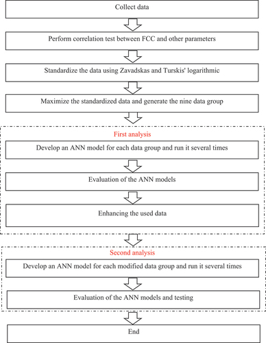
The paper’s methodology consists of several sequential steps: data collection to utilize as data of ANN models, correlation testing to identify the crucial variables, standardization data to obtain suitable results for producing discrepancies between observed and computed results, maximization data to overcome the limit available data, first analysis, and second analysis. The first analysis includes creating ANN models, calculating each developed model’s mean percentage error (MAPE), and removing abnormal data. Furthermore, the second analysis entails creating and running an ANN model on the modified data (without abnormal data) and calculating the MAPE for each ANN model. The methodology flowchart is displayed in Figure 2. The advantage of utilizing the ANN is simplicity and enables dealing with the nominal data such as the sector in this paper. The SPSS IBM program can provide a neat sketch of the use of the ANN model with the strong connection among neurons and the bias values.

Figure 2. Methodology flow chart.

3.1. Data collection

In order to develop models that forecast the FCC of construction projects, we need data from previously completed projects. Collecting data from the completed construction projects in Saudi Arabia was conducted through a survey that was prepared and distributed to several organizations. The survey’s most significant findings are the project classification of the owner’s sector (Public, Semi-Public, or Private) and the type of project in terms of the nature of the work that has been implemented. They were the critical variables required in creating forecast models (buildings, roads, electrical works, mechanical works).

Moreover, the survey’s primary outcomes included the cost of the project upon award (contract cost) and the actual cost of the project after its completion (final construction cost), as well as the project’s scheduled start and end dates (contract duration). After acquiring the data, it was evaluated, and the invalid ones were excluded. The data from 135 projects implemented in Saudi Arabia were suitable for developing and validating models for forecasting a final construction cost (FCC) (Appendix 1). The 135 data distribution in terms of the sector and project type is illustrated in Table 4.

Table 4. Distribution of the collected data.

Project Type Sector	Buildings (1)	Electrical Works (2)	Mechanical Works (3)	Total No. projects
Public (1)	51	11	17	79
Semi-Public (2)	7	43	–	50
Private (3)	6	–	–	6
Total No. projects	64	54	17	135

3.2. Correlation tests between FCC and other parameters

The assumption used in this paper stated that the CC, CD, project sector, and project type affect the change of FFCC of the project. The model’s input parameters should significantly influence the FCC (the output model) to obtain the ANN model with reasonable accuracy. Therefore, the correlation test was carried out between the FCC and input parameters. The input parameters comprise CC, CD, project sector (public, semi-public, and private), and project type (building, electrical, mechanical). Table 5 shows the correlation results between FCC and other parameters; the CC and CD correlate with FCC with a p-value of 0.001 and 0.003, respectively. Moreover, the p-value of the correlation test between FCC and the project sector is 0.06, close to 0.05. on the other hand, there is no correlation between FCC and project type. Therefore, the parameters that can be considered as input layers in the ANN model were CC, CD, and project sector.

Table 5. Correlation test results.

No	Parameters		Pearson correlation	p-value	Number of data
1	FCC	CC	0.999	<0.001	135
2	FCC	CD	0.256	0.003	135
3	FCC	Project Sector	0.19	0.06	135
4	FCC	Project type	0.128	0.137	135

3.3. Data standardization

Anysz, Zbiciak, and Ibadov (2016) examined the 8-normalization method to prepare data integrated into ANN (artificial neural network). They concluded that the Zavadskas and Turskis’ logarithmic method was appropriate for generating errors between the observed and computed outcomes. The Zavadskas and Turskis’ logarithmic formula for standardized input data ($\bar{x}$) or output data ($\overline{y_i}$) is shown in Eq (3)(3) $\overline{x_i}=\frac{Ln\left(x_i\right)}{{\prod }_{i=1}^n{x}_i}$(3) and Eq (4)(4) $\overline{y_i}=\frac{Ln\left(y_i\right)}{{\prod }_{i=1}^n{y}_i}$(4) as:

(3) $\overline{x_i}=\frac{Ln\left(x_i\right)}{{\prod }_{i=1}^n{x}_i}$(3)

(4) $\overline{y_i}=\frac{Ln\left(y_i\right)}{{\prod }_{i=1}^n{y}_i}$(4)

where Ln is a natural logarithm, $x_i$ and $y_i$ represent the input and output data, and n is the total data. In this paper, the $x_i$ was set as $\mathit{C}{C}_i$ or $\mathit{C}{D}_i$, while $y_i$ was set as $\mathit{FC}{C}_i$. Therefore, $\overline{C{C}_i}$ and $\overline{C{D}_i}$ can be obtained using Eq. (1(1) $\mathit{f}=\frac{1-{\mathit{e}}^{-2\mathit{x}}}{1+e^{-2\mathit{x}}}$(1) ), and $\overline{FC{C}_i}$ from Eq (3)(3) $\overline{x_i}=\frac{Ln\left(x_i\right)}{{\prod }_{i=1}^n{x}_i}$(3) . In terms of the sector (independent variable), the variable type is nominal data and can be changed into three options: public (Pub), semi-public (Spub), and private (Pri). The three option was set in the ANN’s input as three impendent variables; “Pub,” “Spub,” and “Pri,” which have two value, one and zero. Therefore, the ANN’ input layer had five variables: $\overline{C{C}_i}$, $\overline{C{D}_i}$, Pub, Spub, and Pri, while the output was $\overline{FC{C}_i}$.

3.4. Maximize the used data

The data used consists of 135 projects and relatively small data. However, the ANN model requires extensive data to provide a reliable forecast. Pasini (2015) established a manner to solve the issue of the relatively small data used in the ANN model. The manner splits all data into the n subgroups. One is set as test data, and the other groups are set as training data. The test data were not considered in the ANN model, while the training data was inserted into ANN as training where the test data percentages of the test and training data are set as 0% and 100%, respectively.

In this paper, the 135 data were divided into ten subgroups. One was considered for testing data and was not inserted into the ANN model. Based on the order test data, the nine-group data were generated, set as training data, and inserted individually into the ANN model, creating the nine ANN models. Therefore, the nine ANN models were developed based on the training data, as shown in Figure 3. In addition, each ANN model had testing data. For example, Tables 6 and 7 are training and testing data for ANN model 1.

Figure 3. Training data distribution for each ANN model.

Table 6. Training data of ANN model 1.

Input parameters					Output parameter
$\overline{\mathit{CC}}$	$\overline{\mathit{CD}}$	Pub	Spub	Pri	$\mathit{F}\overline{\mathit{CD}}$
20.664	13.012	0	1	0	21.626
33.083	0.045	0	1	0	34.148
20.196	12.682	0	1	0	20.940
27.009	14.456	0	1	0	27.879
35.228	15.220	0	1	0	36.341
22.566	14.774	0	1	0	23.293
21.581	16.805	0	1	0	22.276
32.860	15.917	0	1	0	34.512
34.506	14.386	0	1	0	35.623
29.652	14.946	0	1	0	30.607
24.429	14.768	0	1	0	25.216
30.002	14.946	0	1	0	30.896
12.353	11.397	0	1	0	19.563
26.650	16.444	0	1	0	29.370
30.426	14.527	0	2	0	31.405
30.505	15.470	0	1	0	32.055
30.986	15.470	0	1	0	31.969
23.552	13.128	0	1	0	24.311
24.188	14.327	0	1	0	24.765
24.687	14.327	0	1	0	25.473
27.322	14.327	0	1	0	28.195
21.637	14.590	0	1	0	22.535
4.482	14.590	0	1	0	−2.689
20.436	14.590	0	1	0	21.386
10.360	11.434	0	1	0	10.693
10.470	8.114	0	0	0	10.807
14.240	5.067	0	1	0	14.699
26.962	14.590	0	1	0	28.467
29.978	15.611	0	1	0	31.583
25.965	14.590	0	1	0	26.860
26.117	14.590	0	1	0	27.078
25.187	14.590	0	1	0	26.039
11.254	16.265	0	1	0	11.735
18.722	13.270	0	1	0	19.792
17.592	11.043	0	1	0	18.358
22.549	12.418	0	1	0	23.503
42.632	11.359	1	0	0	44.498
30.502	16.381	1	0	0	32.050
29.343	5.022	1	0	0	30.565
16.352	11.359	1	0	0	18.833
29.027	8.556	1	0	0	31.415
29.616	12.759	1	0	0	30.569
14.348	12.063	1	0	0	14.810
20.187	15.547	1	0	0	4.207
17.346	10.961	1	0	0	17.905
−17.224	15.547	1	0	0	−17.779
−10.350	3.168	1	0	0	−10.734
32.553	15.066	1	0	0	33.601
20.418	11.725	1	0	0	21.076
−12.285	3.168	1	0	0	−10.675
24.226	17.085	1	0	0	25.006
8.158	11.359	1	0	0	8.420
−17.072	0.045	1	0	0	−18.523
−10.161	5.022	1	0	0	−10.560
−7.939	0.045	1	0	0	−8.195
22.836	13.212	1	0	0	22.962
−8.164	0.045	1	0	0	−8.427
−15.652	1.853	1	0	0	−16.156
−26.364	0.045	1	0	0	−27.213
−6.858	5.022	1	0	0	−7.079
−9.768	6.337	1	0	0	−10.082
−14.831	0.045	1	0	0	−15.309
−16.066	1.853	1	0	0	−16.592
−4.614	−3.168	1	0	0	−4.918
−4.830	−3.168	1	0	0	−4.987
−8.946	1.853	1	0	0	−9.234
−3.646	8.190	1	0	0	−3.764
−2.438	3.168	1	0	0	−3.401
−4.711	6.337	1	0	0	−4.227
−4.675	6.337	1	0	0	−4.183
−4.803	8.190	1	0	0	−5.480
−4.701	5.022	1	0	0	−4.852
−5.343	5.022	1	0	0	−5.515
16.261	14.129	1	0	0	0.355
−9.606	5.022	1	0	0	−10.676
−8.009	5.022	1	0	0	−8.417
−8.214	3.168	1	0	0	−8.479
−8.258	3.168	1	0	0	−10.794
−8.000	0.045	1	0	0	−8.258
−7.989	0.045	1	0	0	−8.246
−8.260	0.045	1	0	0	−8.526
−9.181	3.168	1	0	0	−9.476
−7.927	3.168	1	0	0	−10.895
−7.925	3.168	1	0	0	−10.713
−15.407	1.853	1	0	0	−15.959
−8.017	3.168	1	0	0	−8.275
−9.671	3.168	1	0	0	−10.347
−7.929	3.168	1	0	0	−8.185
−9.194	8.190	1	0	0	−9.490
−16.958	1.853	1	0	0	−17.549
−4.983	5.022	1	0	0	−5.143
23.108	8.190	1	0	0	23.852
12.781	8.190	1	0	0	12.928
18.244	8.190	1	0	0	18.831
−4.574	5.022	1	0	0	−5.018
−4.857	5.022	1	0	0	−5.217
−5.240	5.022	1	0	0	−5.424
25.743	9.505	0	0	1	27.342
34.529	11.534	0	0	1	36.056
19.714	8.190	0	0	1	20.996
23.396	11.332	0	0	1	25.057
15.780	11.359	0	0	1	16.590
−8.123	0.045	1	0	0	−8.385
−8.877	0.045	1	0	0	−9.163
−8.865	0.045	1	0	0	−9.150
−8.021	−0.332	1	0	0	−8.279
−8.883	−0.332	1	0	0	−9.169
−18.364	0.045	1	0	0	−21.541
−21.967	−3.168	1	0	0	−22.675
−19.714	−3.451	1	0	0	−20.348
−9.927	6.337	1	0	0	−10.246
−15.846	0.045	1	0	0	−16.356
−13.989	5.022	1	0	0	−14.440
−3.435	8.190	1	0	0	−3.546
−13.953	0.045	1	0	0	−17.909
−6.196	3.168	1	0	0	−6.658
27.368	15.623	1	0	0	29.079
25.743	13.275	1	0	0	26.848
21.118	13.275	1	0	0	22.081
33.912	12.063	1	0	0	35.463
40.489	16.381	1	0	0	42.188
33.679	16.381	1	0	0	35.945

Table 7. Testing data of ANN model 1.

Input parameters					Output parameter
$\overline{\mathit{CC}}$	$\overline{\mathit{CD}}$	Pub	Spub	Pri	$\mathit{F}\overline{\mathit{CD}}$
30.281	16.079	0	1	0	31.664
28.233	14.609	0	1	0	29.522
19.638	14.537	0	1	0	20.393
17.647	10.648	0	1	0	18.453
26.914	15.704	0	1	0	28.143
23.744	16.189	0	1	0	24.589
9.732	12.382	0	1	0	10.176
29.683	14.537	0	1	0	31.198
21.196	13.883	0	1	0	22.125
23.630	12.382	0	1	0	24.704
21.990	14.614	0	1	0	22.993
31.388	13.815	0	1	0	33.548
30.820	15.563	0	1	0	32.184
33.128	14.614	0	2	0	34.640

3.5. First analysis

The purpose of the first analysis was to determine the data that may have a detrimental influence on the accurate prediction of the ANN model by carrying out several steps, as shown in the following section.

3.5.1. Develop and run ANN models

After standardization and maximizing data, the ANN model’ structure was performed. The number of hidden layers was two, and the number of neurons per hidden layer was set as (2 m + 1), where m is the number of the input variables (Zayed 2001). Due to the number of variables in the paper being five, the number of neurons was 11 for each hidden layer. The activation function was set as hyperbolic. The ANN model’ structure is shown in Figure 4. The ANN model was run several times. The training process’s relative error (RE) was monitored for each time running and should satisfy the following conditions: 1) the RE shall be less than 10%, and 2) the RE value does not suffer sudden increases. The first condition ensures the accuracy of the model. The second condition avoids the overfitting error (Pasini 2015).

Figure 4. Developed ANN models structure.

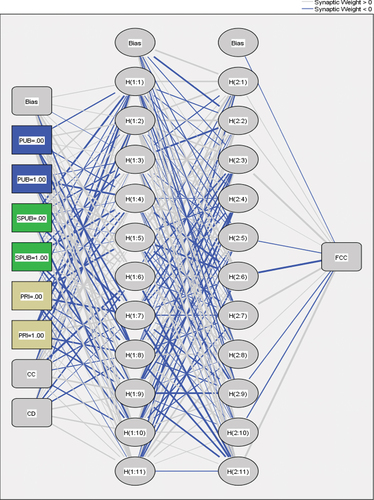
The merits of using ANN in the SPSS IBM program: The program can save the output of the ANN model for each time analysis. Therefore, each ANN model has three set output values that were used to evaluate the model’s accuracy using the mean absolute percentage error MAPE value, as detailed in the following section.

3.5.2. Evaluation of the ANN models

The three output sets (set for each time analysis) of each ANN model were used to compute MAPE using the following steps. The average of the output model was first computed (${\overline{\mathit{FCC}}}_{\mathit{comp}-\mathit{i}}$). Then, the reverse value of the ${\overline{\mathit{FCC}}}_{\mathit{comp}-\mathit{i}}$ was calculated using Eq (2)(2) $\mathit{f}=\frac{1}{1+{\mathit{e}}^{-\mathit{x}}}$(2) and obtained the output computed value of the final construction cost ($\mathit{FC}{C}_{\mathit{comp}-\mathit{i}}$). After that, the MAPE value can be computed using Eq (5)(5) $\mathit{MAPE}=\frac{1}{n}\sum _{\mathit{i}=1}^{\mathit{n}}\frac{\left|\mathit{FC}{\mathit{C}}_{\mathit{obs}-\mathit{i}}-\mathit{FC}{C}_{\mathit{comp}-\mathit{i}}\right|}{\mathit{FC}{C}_{\mathit{obs}-\mathit{i}}}\times 100$(5) .

(5) $\mathit{MAPE}=\frac{1}{n}\sum _{\mathit{i}=1}^{\mathit{n}}\frac{\left|\mathit{FC}{\mathit{C}}_{\mathit{obs}-\mathit{i}}-\mathit{FC}{C}_{\mathit{comp}-\mathit{i}}\right|}{\mathit{FC}{C}_{\mathit{obs}-\mathit{i}}}\times 100$(5)

3.5.3. Enhancing the used data

The ANN model’s data was improved by deleting the abnormal data. Montao Moreno (Montaño Moreno et al. 2013) pointed out that the accuracy models with reasonable forecasting range from 20% to 50%, with an average of 35%. Hence, this value was set as the threshold value for APE to ensure the deletion of abnormal data and obtain a high-accuracy model. For instance, when the case had an APE higher than 35%, the case would be deleted. In addition, if the case had an APE of less than 35%, the case would remain. Therefore, the case that its APE was greater than 35% was considered strange and deleted from the data. The nine modified data groups were generated. The $\mathit{AP}{E}_i$ formula is shown in Eq (6)(6) $\mathit{AP}{E}_i=\frac{\left|\mathit{FC}{\mathit{C}}_{\mathit{obs}-\mathit{i}}-\mathit{FC}{C}_{\mathit{comp}-\mathit{i}}\right|}{\mathit{FC}{C}_{\mathit{obs}-\mathit{i}}}\times 100$(6) :

(6) $\mathit{AP}{E}_i=\frac{\left|\mathit{FC}{\mathit{C}}_{\mathit{obs}-\mathit{i}}-\mathit{FC}{C}_{\mathit{comp}-\mathit{i}}\right|}{\mathit{FC}{C}_{\mathit{obs}-\mathit{i}}}\times 100$(6)

3.6. Second analysis

The second analysis aims to develop the ANN model with high accuracy in predicting the FCC. It was achieved by developing and evaluating the ANN models as illustrated in the first analysis, but the data used were modified. The ANN models were evaluated using MAPE. After that, the ANN models were examined using test data for each model.

The methodology has several implications for the results and outcomes of the model. The method chosen to develop the ANN can impact the accuracy of the predicted final contract cost. Selecting an appropriate method to model the factors influencing the contract cost-effectively is essential to achieve accurate predictions. In addition, the choice of method can be influenced by the availability and quality of the data used to train and validate the ANN. Some methods may require a large amount of high-quality data to effectively capture the underlying relationships and improve the accuracy of the predictions. If there is limited or incomplete data, or if the data quality could be better, it may impact the performance of the chosen method. In this paper, The method used to overcome the limited availability and quality of data.

4. Results and discussions

4.1. Results of the ANN model at the first analysis

The MAPE values of the nine ANN models (at first analysis) that were standardized by Zavadskas and Turskis’ logarithmic standardization method and maximized data method used by (Pasini 2015) are shown in Table 8. The MAPE’s mean, maximum, and minimum values were 18.7%, 20.15%, and 16.78%, respectively.

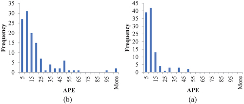
According to R. Gustriansyah, D. I. Sensuse, and A. Ramadhan (2017), the mean MAPE was less than 20% for the classification MAPE value, and the ANN model provided good prediction accuracy. In addition, the frequency of the APE values of the nine models is shown in Table 9. Most of the frequencies were in the range of (0–4.9%) and (5%–9.9%), which reflected the model’s accuracy. However, there were relatively few data points with an APE value of more than 35. These values ranged from 5 to 13 cases, representing 3.7% and 10% of the total data.

Table 8. MAPE value of the nine ANN models with the percentage data that had APE of more than 35% in the first analysis.

Model	MAPE (%)	Percentage data that have anAPE of more than 35%
ANN model 1	20.15	8.8
ANN model 2	17.01	5.9
ANN model 3	17.8	7.8
ANN model 4	16.78	8.14
ANN model 5	17.9	11.11
ANN model 6	17.9	8.8
ANN model 7	17.6	5.9
ANN model 8	18.2	10.3
ANN model 9	19.9	11.11

Table 9. APE Frequencies of the nine ANN models at first analysis.

APE (%)	Frequency
	ANN model 1	ANN model 2	ANN model 3	ANN model 4	ANN model 5	ANN model 6	ANN model 7	ANN model 8	ANN model 9
0–4.9	27	49	50	44	35	42	51	34	40
5–9.9	31	31	26	33	27	38	27	38	23
10–14.9	20	13	15	9	20	10	14	16	22
15–19.9	15	6	5	12	9	7	7	5	8
20–24.9	7	4	4	6	5	3	4	4	6
25–29.9	1	3	3	3	5	2	3	1	2
30–34.9	4	2	3	0	3	5	3	5	2
35–39.9	2	2	2	3	1	3	1	5	3
40–44.9	2	3	3	2	4	3	2	3	4
45–49.9	6	2	3	2	1	2	3	2	3
50–54.9	1	1	3	1	2	0	0	0	1
55–59.9	1	0	0	0	2	0	0	1	0
60–64.9	1	0	0	1	1	1	1	1	1
65–69.9	0	1	0	1	1	0	1	1	0
70–74.9	0	0	0	0	0	1	0	0	0
75–79.9	0	0	0	0	0	0	0	1	0
80–84.9	0	0	0	1	0	0	0	0	0
85–89.9	0	0	0	0	0	0	0	0	0
90–94.9	1	0	0	0	0	0	0	0	0

4.2. Results of ANN models in the second analysis

The data with an APE value of more than 35% in the first analysis were deleted. Then, the nine ANN models were run several times (second analysis). The MAPE values of the nine models were reduced, as shown in Table 8. It ranged from 5.77% to 15.8%, with a mean of 8.7%. Hence, the ANN model provides high accuracy in the prediction of the FCC because the mean of the MAPE (8.7%) was lower than 10%, which was determined by (Gustriansyah, Sensuse, and Ramadhan 2017) to describe the accuracy of the forecasting model. in addition, the percentage of the elimination data was ranged from 5.9% to 11.11%, as shown in Table 8. These percentages were close to 10%, which was reasonable. By examining the deleted data, the results revealed that most of the projects were public projects. There were relationships between the percentage deleted data in Table 8 and the MAPE values in Table 10. For example, the ANN model 2 had a high value of MAPE (15.8%). However, it had the lowest value of the percentage of data deleted (5.9%). In addition, the ANN model 5 had the lowest MAPE value (5.77%) and the highest value of the percentage deleted data (11.1%). The frequency of the APE values that ranged from 15% to 35% in the ANN model 2 was higher than in the ANN model 5, as shown in Figure 5. Hence, these differences affected the MAPE values of the ANN models in the second analysis, and they may lead to preventing a significant reduction in the MAPE. It is worth noting that the APE frequencies shown in Figure 5 were in the first analysis (before deleting the data that had an APE of more than 35%). The higher the MAPE value, the lower the percentage of deleted data.

Table 10. The MAPE values of the nine ANN model conducting the second analysis with the.

Model	ANN model 1	ANN model 2	ANN model 3	ANN model 4	ANN model 5	ANN model 6	ANN model 7	ANN model 8	ANN model 9
MAPE (%)	8.86	15.8	9.8	10.00	5.77	6.10	6.44	8.54	7.60

Figure 5. Frequency of APE a) ANN model 2, b) ANN model 5 was performed in the first analysis.

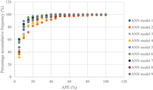
Figure 6 shows the percentage accumulative frequency with absolute percentage error for the nine ANN models in the second analysis. The percentage of data with an APE of 10% or less ranged from 60% to 90% of the used data. In addition, at least 80% of the data had an APE value of 20% or lower. Moreover, Figure 6 revealed that the nine ANN models’ curves followed a unique pattern and that no differences existed among the models.

Figure 6. Percentage accumulative frequency vs. APE for the nine ANN model of the second analysis.

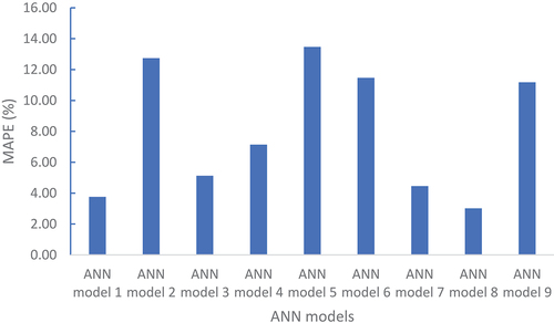
The testing data for each model was used to examine the model’s validity for new data. Figure 7 shows the MAPE of the nine models for test data. The MAPE values vary from 3.01% for ANN model 8 to 13.47% for ANN model 5. These values were less than the allowable (20%) (Gab-Allah, Ibrahim, and Hagras 2015). Hence, the models can predict the FCC with reasonable accuracy.

Figure 7. MAPE of nine models for testing data.

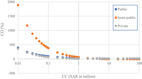
To analyze the results of the ANN model 5, which was more accurate than other models, the ratio of a difference between FCC and CC to CC was examined with CC for different project sectors and several time durations in millions of SAR. This ratio was also called cost overrun, as computed in Eq (7)(7) $\mathit{CO}=\frac{\mathit{FCC}-\mathit{CC}}{\mathit{CC}}\times 100$(7) .

(7) $\mathit{CO}=\frac{\mathit{FCC}-\mathit{CC}}{\mathit{CC}}\times 100$(7)

Figure 8 displays the cost overrun for CD of 3 months; the CO decreases with increasing CC. The private sector project at the CD of 3 months suffers excessive cost overrun for CC ranging from 10,000 SAR to 10,000,000 SAR. However, there is no significant CO for the CC beyond 10,000,000 SAR. Moreover, the public and semi-public project has CO for CC, which changes from 10,000 SAR to 100,000 SAR, as shown in Figure 9. On the other hand, semi-public projects have excessive CO value, with the CO from 660% at a CC of 10,000 SAR to 15.9% at a CC of 1,000,000 SAR. The CO of public and private projects changed from 230% (at a CC of 10,000 SAR) to 29% (at a CC of 1,000,000 SAR). The variance of CO for projects of the three types of sectors for CD of 48 months, as shown in Figure 10, has a similar response.

Figure 8. Cost overrun with contract cost for three sectors at CD of 3 months.

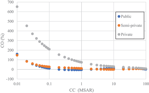
Figure 9. Cost overrun with contract cost for three sectors at CD of 12 months.

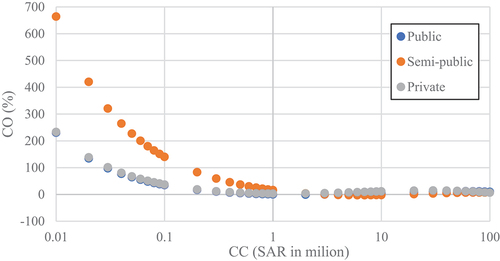
Figure 10. Cost overrun with contract cost for three sectors at CD of 48 months.

4.3. Discussions

The results were discussed in terms of qualitative and quantitative comparisons;

5. Qualitative comparisons

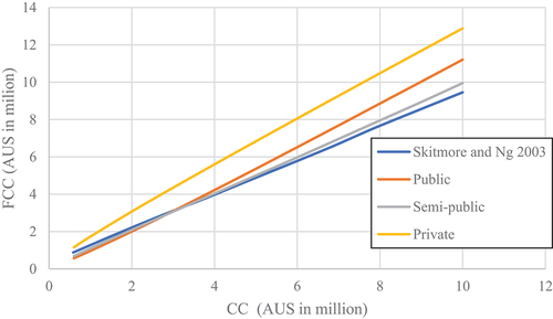
The results models developed by Skitmore & Ng (2003) were considered for comparison with the results of the ANN model. Figure 11 shows the FCC versus CC curve for a contract duration of 100 days for a residential building project. The type contract of the curve was a lump sum. The type of contractor selection was open tendering. The ANN model was utilized to generate FCC-CC curves for the three types of sectors and CD of 100 days (3.33 months). It is clear from Figure 11 that the curve of the semi-government sector is mainly identical to the curve calculated from Skitmore and Ng’s (2003) study. While the curve of the public sector corresponds to the curve of the previous study for a contract value ranging from half a million Australian dollars to four million Australian dollars, the difference between them increases whenever the contract cost value exceeds four million.

The CO of the public project was close to 10%. This percentage is because the Saudi public project limits the order increase by 10% and not reduced by 20%. On the other hand, the private sector curve is far from the study curve and suffers from a significant cost overrun. The contractors in the private sector tend to get more profit from the construction project. Private initiatives are carried out by businesses looking to optimize their returns on investment; they are frequently motivated by financial considerations. The direct construction expenses and the private entity’s profit margins are included in the total contract price. This profit margin increases the total cost of the project. A competitive bidding process where contractors submit offers to win the project is also frequently used for private projects. Contractors may add a premium in their bids to account for uncertainties, risks, or prospective changes in project requirements, which might increase the cost of the contract as a result of the bidding process. The cost of the contract may increase as a result of this market competition. Additionally, private initiatives may have shorter schedules than public projects due to the necessity to make profits or satisfy specific economic objectives. Accelerated Construction schedules result in more significant expenses because contractors may need to hire more staff, work longer hours, or buy materials more quickly. All of these factors can raise the price of a contract.

van den Hurk et al. (2022) stated the importance of improving the private sector skills to reduce the financial risks with accepted delivering profits for the private sector. Based on the data in the specified Figure 11, it is noted that the increase in cost overrun in Saudi Arabia is slightly more significant than in Australia and increases if the value of the contract cost exceeds four million Australian dollars.

Figure 11. FCC vs. CC for three sectors with curve obtained by skitmore and Ng for CD of 100 days.

6. Quantitative comparisons

To compare the accuracy of the ANN models with models developed in the previous studies, the neural model developed by Alcineide et al. (2021) based on artificial neural networks resulted in an average percentage error between 5 and 9%. Elmousalami (2020) has also expressed that the MAPE of the XGBoost model was 9.091%. The mean absolute percentage errors of the developed ANN models are 8.7%, smaller than the MAPE values of the two previous models. In addition, Aibinu et al. (2015) illustrated the effectiveness of machine learning techniques, mainly cost prediction of electrical facilities also researched. Their findings agreed with this paper’s results regarding the accuracy of the ANN model from the MLR model. In comparison with previous studies, it is very reasonable. The ANN model with standardized data utilized by Zavadskas and Turskis’ logarithmic method (Anysz, Zbiciak, and Ibadov 2016) and maximized data using the method introduced by Pasini (2015) provides an average MAPE value of 18.7%. By incorporating the method of removing data with an APE greater than 35%, the MAPE of the ANN model is reduced to 8.7% on average.

6.1. Practical and theoretical implications of the ANN model

The ANN model can support scenario analysis and optimization processes. Decision-makers can enter different scenarios into the model to evaluate how they will affect the final contract cost. This method aids in identifying economic choices and streamlining project schedules. As an illustration, a civil engineering company is debating between two bridge designs for a highway project. The company may evaluate the financial effects of each design by expressing CC and CD in the ANN model, considering things like material costs, construction complexity, and maintenance needs. It allows the company to choose the design that meets the project requirements while minimizing the contract cost.

The ANN model can provide more accurate cost estimates for construction projects. The model can learn the relationships between these factors and the final contract cost by training the model on historical project data, including factors. The model enables decision-makers to have a more precise estimate of the project cost, allowing for better budgeting and resource allocation. For instance, a construction company is bidding on a new highway project. Using an ANN model trained on historical data, the company can input the project specifications into the model and obtain an estimated contract cost. This information helps the company decide whether to proceed with the bid and at what price.

In conclusion, the ANN model has two advantages. The first advantage is the possibility of using relatively little data to train and test any ANN model. The second advantage is to predict the FCC based on three common characteristics of the project (CC, CD, and Project sector).

7. Conclusions

The paper utilized the 135 King Saud University construction projects to develop the artificial neural network (ANN) to predict the final construction cost (FCC) based on the contract cost (CC), contract duration (CD), and project sector. The data were first standardized using Zavadskas and Turskis’ logarithmic method. Then, the standardized data were maximized using the method introduced by Pasini Liu (2013) to overcome the issues of the relatively small data, where the 135 data were divided into ten subgroups; one of them was set as testing data, which was not considered the ANN model. Based on the order testing data, the nine data groups were generated. Each data group represents 90% of the total data and is utilized in the ANN model as complete training data, where the testing data was set to zero. The nine ANN models were run several times to monitor the relative error each time and avoid the overfitting error. After that, the average percentage error (APE) was computed based on the computed FCC from the ANN model and observed FCC. Based on the computed FCC and observed FCC and for each training data group, the absolute percentage error (APE) was computed throughout the training data. For each of the nine training data groups, the training data were enhanced by deleting data with an APE value of more than 35% and generating the modified training data. Finally, the ANN model was developed based on the modified training data. The results revealed that the ANN model provides the MAPE value of 18.7% with standardized data using the logarithmic technique proposed by Zavadskas and Turskis and maximized data using the method proposed by (Pasini 2015). The MAPE of the ANN model is decreased to 8.7% on average by deleting data with an APE greater than 35%. The ANN model has outperformed the FCC prediction of the different linear regression models. Decision-makers will benefit from using these forecasting models to help them assess the viability of construction projects, plan how they will be carried out, keep an eye on how they are doing, and make wiser choices. The developed model was recommended to improve by inserting several crucial risks as input variables. In addition, the limitation of the paper is that it does not consider the interdependencies among the three input variables. In addition, the model depends on the historical data. However, construction projects are subject to evolving technologies, methodologies, and market conditions that may render the historical data less relevant. The model may need help to adapt to changing trends and dynamics accurately. Therefore, more studies were required to capture these interdependencies. The benefit of ANN models for forecasting final contract costs in construction projects can have significant broader impacts, including enhanced cost accuracy, improved cost control, informed decision-making, and project performance evaluation.

Disclosure statement

No potential conflict of interest was reported by the author(s).

Data availability statement

The raw data supporting the findings of this paper are available on request from the corresponding author.

Additional information

Funding

The authors thank the Deputyship for Research and Innovation, Ministry of Education in Saudi Arabia, for funding this research work through project no. [IFKSUOR3-380-8].

Appendix. Raw data

Table

No.	Contract cost (CC) (SAR)	Contract duration (CD) (Month)	Final construction cost (FCC) (SAR)	Public	Semi-public	PRIVATE
1	1,500,000	138.3	1,500,000	0	1	0
2	68,460,000	33	68,460,000	0	1	0
3	51,438,229	23.97	51,438,229	0	1	0
4	15,499,528	23.6	15,209,528	0	1	0
5	11,739,569	10.13	11,739,569	0	1	0
6	42,791,190	30.42	42,791,190	0	1	0
7	27,490,435	33.8	26,629,534	0	1	0
8	3,889,500	14.77	3,889,500	0	1	0
9	62,974,880	23.6	64,339,880	0	1	0
10	19,265,430	20.47	19,165,150	0	1	0
11	27,058,829	14.77	27,040,098	0	1	0
12	21,520,394	24	21,520,394	0	1	0
13	79,890,345	20.17	88,039,533	0	1	0
14	73,802,382	29.5	73,385,052	0	1	0
15	23,106,764	17.23	24,137,303	0	1	0
16	1.53E+08	1	152,539,013	0	1	0
17	21,520,394	16.03	21,818,706	0	1	0
18	60,606,426	23.63	60,606,426	0	1	0
19	2.11E+08	27.93	210,658,262	0	1	0
20	30,851,600	25.33	30,851,600	0	1	0
21	26,562,763	39.5	26,562,763	0	1	0
22	1.47E+08	32.53	160,931,252	0	1	0
23	1.89E+08	23.27	189,512,857	0	1	0
24	90,562,500	26.3	90,562,500	0	1	0
25	40,948,000	25.3	40,948,000	0	1	0
26	95,500,000	26.3	94,502,135	0	1	0
27	6,535,200	12.1	17,817,300	0	1	0
28	57,382,472	36.5	75,482,472	0	1	0
29	1.02E+08	24	101,852,500	0	2	0
30	1.03E+08	29.5	112,084,608	0	1	0
31	1.11E+08	29.5	110,676,272	0	1	0
32	35,840,000	17.67	35,840,000	0	1	0
33	39,473,010	22.97	38,320,524	0	1	0
34	42,585,725	22.97	42,527,615	0	1	0
35	63,554,955	22.97	63,496,845	0	1	0
36	26,787,515	24.33	27,595,392	0	1	0
37	1,976,113	24.33	673,129	0	1	0
38	22,321,935	24.33	23,300,970	0	1	0
39	4,827,143	12.2	4,827,143	0	1	0
40	4,908,491	5.9	4,908,491	0	0	0
41	8,705,670	3.03	8,705,670	0	1	0
42	60,170,000	24.33	66,091,938	0	1	0
43	95,154,746	30.42	104,556,133	0	1	0
44	51,711,016	24.33	52,165,996	0	1	0
45	52,922,740	24.33	53,862,307	0	1	0
46	45,947,586	24.33	46,224,275	0	1	0
47	5,530,000	35.1	5,627,067	0	1	0
48	17,202,401	18.23	18,427,992	0	1	0
49	14,486,980	11.2	14,919,245	0	1	0
50	30,771,774	15.13	31,822,087	0	1	0
51	6.51E+08	12	700,000,000	1	0	0
52	1.03E+08	36	112,000,000	1	0	0
53	86,400,000	3	90,000,000	1	0	0
54	12,000,000	12	16,000,000	1	0	0
55	82,351,564	6.5	102,000,000	1	0	0
56	90,060,950	16.3	90,060,950	1	0	0
57	8,850,000	14	8,850,000	1	0	0
58	21,491,170	30	1,857,617	1	0	0
59	13,957,188	11	13,957,188	1	0	0
60	72,990	30	72,990	1	0	0
61	207,475	2	205,915	1	0	0
62	1.41E+08	27	140,726,856	1	0	0
63	22,259,958	13	22,259,958	1	0	0
64	154,600	2	207,706	1	0	0
65	39,704,154	42	39,704,154	1	0	0
66	3,454,386	12	3,454,386	1	0	0
67	74,700	1	65,420	1	0	0
68	213,500	3	211,265	1	0	0
69	299,250	1	299,250	1	0	0
70	32,142,222	18	29,386,340	1	0	0
71	289,217	1	289,217	1	0	0
72	92,694	1.5	92,694	1	0	0
73	18,200	1	18,200	1	0	0
74	352,685	3	352,685	1	0	0
75	226,653	4	226,653	1	0	0
76	105,000	1	105,000	1	0	0
77	87,034	1.5	86,919	1	0	0
78	496,000	0.5	484,800	1	0	0
79	480,000	0.5	479,856	1	0	0
80	256,800	1.5	256,800	1	0	0
81	574,590	6	574,590	1	0	0
82	690,450	2	606,125	1	0	0
83	488,775	4	536,701	1	0	0
84	491,400	4	540,225	1	0	0
85	481,950	6	446,326	1	0	0
86	489,510	3	489,510	1	0	0
87	444,000	3	444,000	1	0	0
88	11,835,120	22	1,053,688	1	0	0
89	232,281	3	207,678	1	0	0
90	296,100	3	289,620	1	0	0
91	287,000	2	287,000	1	0	0
92	285,100	2	204,100	1	0	0
93	296,500	1	296,500	1	0	0
94	297,000	1	297,000	1	0	0
95	285,000	1	285,000	1	0	0
96	247,800	2	247,800	1	0	0
97	299,810	2	201,086	1	0	0
98	299,907	2	206,554	1	0	0
99	96,200	1.5	95,420	1	0	0
100	295,750	2	295,750	1	0	0
101	230,000	2	218,000	1	0	0
102	299,700	2	299,700	1	0	0
103	247,300	6	247,300	1	0	0
104	76,000	1.5	75,500	1	0	0
105	469,000	3	469,000	1	0	0
106	33,500,000	6	33,500,000	1	0	0
107	6,974,000	6	6,707,640	1	0	0
108	15,996,979	6	15,996,979	1	0	0
109	499,000	3	477,724	1	0	0
110	478,000	3	463,885	1	0	0
111	451,000	3	450,000	1	0	0
112	50,000,000	8	56,000,000	0	0	1
113	1.9E+08	12.47	202,000,000	0	0	1
114	20,000,000	6	22,000,000	0	0	1
115	35,000,000	11.93	40,000,000	0	0	1
116	11,000,000	12	11,500,000	0	0	1
117	291,000	1	291,000	1	0	0
118	259,500	1	259,500	1	0	0
119	260,000	1	260,000	1	0	0
120	295,576	0.93	295,576	1	0	0
121	259,259	0.93	259,259	1	0	0
122	61,380	1	41,950	1	0	0
123	35,500	0.5	35,500	1	0	0
124	50,000	0.47	50,000	1	0	0
125	221,250	4	221,250	1	0	0
126	90,000	1	90,000	1	0	0
127	119,333	3	119,333	1	0	0
128	593,295	6	593,295	1	0	0
129	120,000	1	71,600	1	0	0
130	390,000	2	375,228	1	0	0
131	64,000,000	30.5	72,320,000	1	0	0
132	49,998,494	18.25	52,068,214	1	0	0
133	24,756,246	18.25	25,811,223	1	0	0
134	1.73E+08	14	185,110,000	1	0	0
135	4.7E+08	36	498,200,000	1	0	0

References

- Aamodt, A., and E. Plaza. 1994. “Case-based Reasoning: Foundational Issues, Methodological Variations, and System Approaches.” AI Communications 7 (1): 39–59. https://doi.org/10.3233/AIC-1994-7104.
- Acebes, F., M. Pereda, D. Poza, J. Pajares, and J. M. Galán. 2015. “Stochastic Earned Value Analysis Using Monte Carlo Simulation and Statistical Learning Techniques.” International Journal of Project Management 33 (7): 1597–1609. https://doi.org/10.1016/j.ijproman.2015.06.012.
- Aibinu, A. A., D. Dassanayake, T. K. Chan, and R. Thangaraj. 2015. “Cost Estimation for Electric Light and Power Elements during Building Design: A Neural Network Approach.” Engineering, Construction and Architectural Management 22 (2): 190–213. https://doi.org/10.1108/ECAM-01-2014-0010.
- Aidan, I. A., D. Al-Jeznawi, and F. M. S. Al-Zwainy. 2020. “Predicting Earned Value Indexes in Residential Complexes’ Construction Projects Using Artificial Neural Network Model.” International Journal of Intelligent Engineering and Systems 13 (4): 248–259. https://doi.org/10.22266/IJIES2020.0831.22.
- Alcineide, P., S. Gean, M. F. M. Luiz, C. A. Felipe, and D. G. S. Débora. 2021. “Cost Forecasting of Public Construction Projects Using Multilayer Perceptron Artificial Neural Networks: A Case Study.” Ingenieria e Investigacion 41 (3). https://doi.org/10.15446/ing.investig.v41n3.87737.
- Algahtany, M., Y. Alhammadi, and D. Kashiwagi. 2016. “Introducing a New Risk Management Model to the Saudi Arabian Construction Industry.” Procedia Engineering 145: 940–947. https://doi.org/10.1016/j.proeng.2016.04.122.
- Almasabha, G., K. F. Al-Shboul, A. Shehadeh, and O. Alshboul. 2023. “Machine learning-Based Models for Predicting the Shear Strength of Synthetic fiber-Reinforced Concrete Beams without Stirrups.” Structures 52: 299–311. https://doi.org/10.1016/j.istruc.2023.03.170.
- AlMunif, A. A., and S. Almutairi. 2021. “Lessons Learned Framework for Efficient Delivery of Construction Projects in Saudi Arabia.” Construction Economics and 21(4). Building. https://doi.org/10.3316/informit.321301288812719.
- Alshboul, O., G. Almasabha, A. Shehadeh, R. E. A. Mamlook, A. S. Almuflih, and N. Almakayeel. 2022. “Machine Learning-Based Model for Predicting the Shear Strength of Slender Reinforced Concrete Beams without Stirrups.” Buildings 12 (8): 1166. https://doi.org/10.3390/buildings12081166.
- Alshboul, O., A. Shehadeh, R. E. A. Mamlook, G. Almasabha, A. S. Almuflih, and S. Y. Alghamdi. 2022. “Prediction Liquidated Damages via Ensemble Machine Learning Model: Towards Sustainable Highway Construction Projects.” Sustainability 14 (15): 9303. https://doi.org/10.3390/su14159303. Sustainability (Switzerland), 14(15).
- Alsugair, A. M. 2022. “Cost Deviation Model of Construction Projects in Saudi Arabia Using PLS-SEM.” Sustainability 14 (24): 16391. https://doi.org/10.3390/su142416391.
- Alzara, M., J. Kashiwagi, and A. Al-Tassan. 2018. “Analysis of Cost Overruns in Saudi Arabia Construction Projects: A University Case Study Journal for the Advancement of Performance Information and Value 10 1:84–101.
- Antoniadis, P. 2023. Activation Functions: Sigmoid Vs Tanh. Baeldung. Accessed March 16, 2023. https://www.baeldung.com/cs/sigmoid-vs-tanh-functions.
- Anysz, H., A. Zbiciak, and N. Ibadov. 2016. “The Influence of Input Data Standardization Method on Prediction Accuracy of Artificial Neural Networks.” Procedia Engineering 153: 66–70. https://doi.org/10.1016/j.proeng.2016.08.081.
- Aretoulis, G. N. 2019. “Neural Network Models for Actual Cost Prediction in Greek Public Highway Projects.” International Journal of Project Organisation and Management 11 (1): 41. https://doi.org/10.1504/ijpom.2019.10019946.
- Aria, M., C. Cuccurullo, and A. Gnasso. 2021. “A Comparison among Interpretative Proposals for Random Forests.” Machine Learning with Applications 6: 100094. https://doi.org/10.1016/j.mlwa.2021.100094.
- Badawy, M. 2020. “A Hybrid Approach for A Cost Estimate of Residential Buildings in Egypt at the Early Stage.” Asian Journal of Civil Engineering 21 (5): 763–774. https://doi.org/10.1007/s42107-020-00237-z.
- Badawy, M., F. Alqahtani, and H. Hafez. 2022. “Identifying the Risk Factors Affecting the Overall Cost Risk in Residential Projects at the Early Stage.” Ain Shams Engineering Journal 13 (2): 101586. https://doi.org/10.1016/j.asej.2021.09.013.
- Baek, M., D. Ph, B. Ashuri, and D. Ph. 2019. “Assessing Low Bid Deviation from Engineer’s Estimate in Highway Construction Projects.” Denver: Associated Schools of Construction 2013: 371–377.
- Bayram, S., and S. Al-Jibouri. 2016. “Efficacy of Estimation Methods in Forecasting Building Projects’ Costs.” Journal of Construction Engineering and Management 142 (11): 05016012. https://doi.org/10.1061/(ASCE)CO.1943-7862.0001183.
- Bilal, M., L. O. Oyedele, J. Qadir, K. Munir, S. O. Ajayi, O. O. Akinade, H. A. Owolabi, H. A. Alaka, and M. Pasha. 2016. “Big Data in the Construction Industry: A Review of Present Status, Opportunities, and Future Trends.” In Advanced Engineering Informatics. 30 (3): Elsevier , 500–521. https://doi.org/10.1016/j.aei.2016.07.001.
- Breiman, L. 2001. “Random Forests.” Machine learning 45:5–32.
- Castro Miranda, S. L., E. Del Rey Castillo, V. Gonzalez, and J. Adafin. 2022. “Predictive Analytics for Early-Stage Construction Costs Estimation.” In Buildings, 1043. Vol. 12. https://doi.org/10.3390/buildings12071043.
- Chakraborty, D., H. Elhegazy, H. Elzarka, and L. Gutierrez. 2020. “A Novel Construction Cost Prediction Model Using Hybrid Natural and Light Gradient Boosting.” Advanced Engineering Informatics 46:101201. https://doi.org/10.1016/j.aei.2020.101201.
- Cheki, M., H. Jazayeri-Rad, and P. Karimi. 2016. “Enhancing the Noise Tolerance of Fault Diagnosis System Using the Modified Adaptive Boosting Algorithm.” Journal of Natural Gas Science and Engineering 29: 303–310. https://doi.org/10.1016/j.jngse.2015.12.029.
- Chen, H. L., W. T. Chen, and Y. L. Lin. 2016. “Earned Value Project Management: Improving the Predictive Power of Planned Value.” International Journal of Project Management 34 (1): 22–29. https://doi.org/10.1016/j.ijproman.2015.09.008.
- Chen, T., and C. Guestrin (2016). “Xgboost: A Scalable Tree Boosting System.” In Proceedings of the 22nd Acm Sigkdd International Conference on Knowledge Discovery and Data Mining, New York, 785–794.
- Curram, S. P., and J. Mingers. 1994. “Neural Networks, Decision Tree Induction and Discriminant Analysis: An Empirical Comparison.” Journal of the Operational Research Society 45 (4): 440–450. https://doi.org/10.1057/jors.1994.62.
- Dietterich, T. G., and E. B. Kong. 1995. “Machine Learning Bias, Statistical Bias, and Statistical Variance of Decision Tree Algorithms.” https://citeseerx.ist.psu.edu/document?repid=rep1&type=pdf&doi=893b204890394d1bf4f3332b4b902bfdb30a9a13.
- Elhegazy, H., N. Badra, S. A. Haggag, and I. Abdel Rashid. 2022. “Implementation of the Neural Networks for Improving the Projects’ Performance of Steel Structure Projects.” Journal of Industrial Integration and Management 70 (1): 133–152. https://doi.org/10.1142/S2424862221500251.
- Elhegazy, H., D. Chakraborty, H. Elzarka, A. M. Ebid, I. M. Mahdi, S. Y. Aboul Haggag, and I. Abdel Rashid. 2022. “Artificial Intelligence for Developing Accurate Preliminary Cost Estimates for Composite Flooring Systems of Multi-Storey Buildings.” Journal of Asian Architecture and Building Engineering 21 (1): 120–132. https://doi.org/10.1080/13467581.2020.1838288.
- Elmousalami, H. H. 2020. “Artificial Intelligence and Parametric Construction Cost Estimate Modeling: State-Of-The-Art Review.” Journal of Construction Engineering and Management 146 (1): 03119008. https://doi.org/10.1061/(ASCE)CO.1943-7862.0001678.
- Espinosa-Garza, G., and I. Loera-Hernández. 2017. “Proposed Model to Improve the Forecast of the Planned Value in the Estimation of the Final Cost of the Construction Projects.” Procedia Manufacturing 13: 1011–1018. https://doi.org/10.1016/j.promfg.2017.09.103.
- Flyvbjerg, B., M. S. Holm, and S. Buhl. 2002. “Underestimating Costs in Public Works Projects: Error or Lie?” Journal of the American Planning Association 68 (3): 279–295. https://doi.org/10.1080/01944360208976273.
- Gab-Allah, A. A., A. H. Ibrahim, and O. A. Hagras. 2015. “Predicting the Construction Duration of Building Projects Using Artificial Neural Networks.” International Journal Applied Management Science 7 (2): 123–141.
- Gao, X., and P. Pishdad-Bozorgi. 2020. “A Framework of Developing Machine Learning Models for Facility life-Cycle Cost Analysis.” Building Research and Information 48 (5): 501–525. https://doi.org/10.1080/09613218.2019.1691488.
- Gustriansyah, R., D. I. Sensuse, and A. Ramadhan. 2017. “A Sales Prediction Model Adopted the recency-Frequency-Monetary Concept.” Indonesian Journal of Electrical Engineering and Computer Science 6 (3): 711–720. https://doi.org/10.11591/ijeecs.v6.i3.,711-720.
- Heralova, R. S. 2017. “Life Cycle Costing as an Important Contribution to Feasibility Study in Construction Projects.” Procedia Engineering 196: 565–570. https://doi.org/10.1016/j.proeng.2017.08.031.
- Kim, B.-C., and K. F. Reinschmidt. 2011. “Combination of Project Cost Forecasts in Earned Value Management.” Journal of Construction Engineering and Management 137 (11): 958–966. https://doi.org/10.1061/(asce)co.1943-7862.0000352.
- Leon, H., H. Osman, M. Georgy, and M. Elsaid. 2018. “System Dynamics Approach for Forecasting Performance of Construction Projects.” Journal of Management in Engineering 34 (1). https://doi.org/10.1061/(asce)me.1943-5479.0000575.
- Liu, Z. 2013. “Design of Foundations for Large Dynamic Equipment in a High Seismic Region.” Structures Congress 2013: Bridging Your Passion with Your Profession 1403–1414.
- Li, M., Q. Zheng, and B. Ashuri. 2022. “Predicting Ratio of Low Bid to Owner’s Estimate Using Feedforward Neural Networks for Highway Construction.” Construction Research Congress 2022: 340–350.
- Love, P. E. D., D. J. Edwards, S. Han, and Y. M. Goh. 2011. “Design Error Reduction: Toward the Effective Utilization of Building Information Modeling.” Research in Engineering Design 22 (3): 173–187. https://doi.org/10.1007/s00163-011-0105-x.
- Lowe, D. J. (2006). Predicting Construction Cost Using Multiple Regression Techniques. Cite This Paper. https://doi.org/10.1061/(ASCE)0733.
- Loy, J. 2019. Neural Network Projects with Python: The Ultimate Guide to Using Python to Explore the True Power of Neural Networks through Six Projects. Packt Publishing.
- Mahamid, I. 2018. “Critical Determinants of Public Construction Tendering Costs.” International Journal of Architecture, Engineering and Construction 7 (1). https://doi.org/10.7492/ijaec.2018.005.
- Marín-Veites, P., and K. Bach (2022). “Explaining CBR Systems through Retrieval and Similarity Measure Visualizations: A Case Study.” In International Conference on Case-Based Reasoning, 111–124.
- Mir, M., H. M. D. Kabir, F. Nasirzadeh, and A. Khosravi. 2021. “Neural network-Based Interval Forecasting of Construction Material Prices.” Journal of Building Engineering 39:102288. https://doi.org/10.1016/j.jobe.2021.102288.
- Moghayedi, A., and A. Windapo. 2021. Predicting the Impact Size of Uncertainty Events on Construction Cost and Time of Highway Projects Using ANFIS Technique.” In Collaboration and Integration in Construction, Engineering, Management and Technology: Proceedings of the 11th International Conference on Construction in the 21st Century, London, 2019, 203–209. Cham: Springer.
- Mohammadifardi, H., M. A. Knight, and A. A. J. Unger. 2019. “Sustainability Assessment of Asset Management Decisions for Wastewater Infrastructure systems – Implementation of a System Dynamics Model.” Systems 7 (3): 34. https://doi.org/10.3390/systems7030034.
- Montaño Moreno, J. J., A. Palmer Pol, A. Sesé Abad, and B. Cajal Blasco. 2013. “El índice R-MAPE como medida resistente del ajuste en la previsiońn.” Psicothema 25 (4): 500–506. https://doi.org/10.7334/psicothema2013.23.
- Natarajan, A. 2022. “Reference Class Forecasting and Machine Learning for Improved Offshore Oil and Gas Megaproject Planning: Methods and Application.” Project Management Journal 53 (5): 456–484. https://doi.org/10.1177/87569728211045889.
- Ng, S. T., S. O. Cheung, M. Skitmore, and T. C. Y. Wong. 2004. “An Integrated Regression Analysis and Time Series Model for Construction Tender Price Index Forecasting.” Construction Management and Economics 22 (5): 483–493. https://doi.org/10.1080/0144619042000202799.
- Ngo, J., B. G. Hwang, and C. Zhang 2020. “Big Data and Predictive Analytics in the Construction Industry: Applications, Status Quo, and Potential in Singapore’s Construction Industry.” In Construction Research Congress 2020, 715–724. Reston, VA: American Society of Civil Engineers.
- Ngo, K. A., G. Lucko, and P. Ballesteros-Pérez. 2022. Continuous Earned Value Management with Singularity Functions for Comprehensive Project Performance Tracking and Forecasting. Automation in Construction, 143. https://doi.org/10.1016/j.autcon.2022.104583.
- Odeyinka, H., J. Lowe, and A. Kaka. 2012. “Regression Modelling of Risk Impacts on Construction Cost Flow Forecast.” Journal of Financial Management of Property and Construction 17 (3): 203–221. https://doi.org/10.1108/13664381211274335.
- Olawale, Y. A., and M. Sun. 2010. “Cost and Time Control of Construction Projects: Inhibiting Factors and Mitigating Measures in Practice.” Construction Management and Economics 28 (5): 509–526. https://doi.org/10.1080/01446191003674519.
- Osuna, E., and F. Girosi. 1998. “Reducing the Run-Time Complexity of Support Vector Machines.” In International Conference on Pattern Recognition.
- Pasini, A. 2015. “Artificial Neural Networks for Small Dataset Analysis.” Journal of Thoracic Disease 7 (5): 953–960. https://doi.org/10.3978/j.2072-1439.2015.04.61.
- Pasini, A., M. Lorè, and F. Ameli. 2006. “Neural Network Modelling for the Analysis of forcings/temperatures Relationships at Different Scales in the Climate System.” Ecological Modelling 191 (1): 58–67. https://doi.org/10.1016/j.ecolmodel.2005.08.012.
- Perner, P., U. Zscherpel, and C. Jacobsen. 2001. “A Comparison between Neural Networks and Decision Trees Based on Data from Industrial Radiographic Testing.” Pattern Recognition Letters 22 (1): 47–54. https://doi.org/10.1016/S0167-8655(00)00098-2.
- Prasad, A. M., L. R. Iverson, and A. Liaw. 2006. “Newer Classification and Regression Tree Techniques: Bagging and Random Forests for Ecological Prediction.” Ecosystems 9 (2): 181–199. https://doi.org/10.1007/s10021-005-0054-1.
- Qin, C., Y. Zhang, F. Bao, C. Zhang, P. Liu, P. Liu, and S. B. Kotsiantis. 2021. “XGBoost Optimized by Adaptive Particle Swarm Optimization for Credit Scoring.” Mathematical Problems in Engineering 2021:1–18. https://doi.org/10.1155/2021/6655510.
- Sackey, S., D. E. Lee, and B. S. Kim. 2020. “Duration Estimate at Completion: Improving Earned Value Management Forecasting Accuracy.” KSCE Journal of Civil Engineering 24 (3): 693–702. https://doi.org/10.1007/s12205-020-0407-5.
- Saqer, F., Y. Malalla, P. S. M. A. Suliman, and O. A. Jamal. 2020. “Development of Cost Estimation Model for Ministry of Youth and Sports Affairs Construction Projects A Case Study from Kingdom of Bahrain Submitted By : Supervised by May .
- Schapire, R. E. 1990. “The Strength of Weak Learnability.” Machine learning 5:197–227.
- Shehadeh, A., O. Alshboul, R. E. Al Mamlook, and O. Hamedat. 2021. “Machine Learning Models for Predicting the Residual Value of Heavy Construction Equipment: An Evaluation of Modified Decision Tree, LightGBM, and XGBoost Regression.” Automation in Construction 129:103827. https://doi.org/10.1016/j.autcon.2021.103827.
- Skitmore, R. M., and S. T. Ng. 2003. “Forecast Models for Actual Construction Time and Cost.” Building and Environment 38 (8): 1075–1083. https://doi.org/10.1016/S0360-1323(03)00067-2.
- Tayefeh Hashemi, S., O. M. Ebadati, and H. Kaur. 2020. “Cost Estimation and Prediction in Construction Projects: A Systematic Review on Machine Learning Techniques.” SN Applied Sciences. 2. Springer Nature. https://doi.org/10.1007/s42452-020-03497-1.
- Thomas, N., and A. V. Thomas. 2016. “Regression Modelling for Prediction of Construction Cost and Duration.” Applied Mechanics and Materials 857: 195–199. https://doi.org/10.4028/www.scientific.net/amm.857.195.
- van den Hurk, M., D. Williams, A. Luis Dos Santos Pereira, and A. Tallon. 2022. “Brownfield Regeneration and the Shifting of Financial Risk: Between Plans and Reality in public-Private Partnerships.” Urban Research and Practice 1–22. https://doi.org/10.1080/17535069.2022.2144430.
- Vapnik, V. 2006. Estimation of Dependences Based on Empirical Data. Springer Science & Business Media.
- Vinayagam, R., N. Dave, T. Varadavenkatesan, N. Rajamohan, M. Sillanpää, A. K. Nadda, M. Govarthanan, and R. Selvaraj. 2022. “Artificial Neural Network and Statistical Modelling of Biosorptive Removal of Hexavalent Chromium Using Macroalgal Spent Biomass.” Chemosphere 296. https://doi.org/10.1016/j.chemosphere.2022.133965.
- Wu, Z., and J. Xu. 2013. “Predicting and Optimization of Energy Consumption Using System dynamics-Fuzzy Multiple Objective Programming in World Heritage Areas.” Energy 49: 19–31. https://doi.org/10.1016/j.energy.2012.10.030.
- Xu, C., Y. Wang, K. Ye, S. Zhang, M. Zou, and C. Chen (2019). “Research on Transmission Line Project Cost Forecast Method Based on BP Neural Network.” IOP Conference Series: Materials Science and Engineering, 688(5). https://doi.org/10.1088/1757-899X/688/5/055074.
- Ye, D. 2021. “An Algorithm for Construction Project Cost Forecast Based on Particle Swarm Optimization-Guided Bp Neural Network.” Scientific Programming 2021. https://doi.org/10.1155/2021/4309495.
- Zadeh, L. A. 1976. “The Concept of Linguistic Variable and Its Application to Approximate reasoning-III.” Information Sciences 9 (1): 43–80. https://doi.org/10.1016/0020-0255(75)90017-1.
- Zayed, T. 2001. “Assessment of Productivity for Concrete Bored Pile Construction.” Doctoral dissertation, Purdue University.