Spatiotemporal evolution of carbon emissions and influencing factors in county-level based on nighttime lighting data: a case study in Huaihai economic zone core city

ABSTRACT

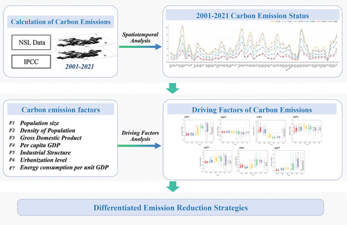
Driven by China’s carbon peaking and carbon neutrality goals, this study constructs a carbon emission inversion model for 57 county-level in the core city cluster of the Huaihai Economic Zone. It analyzes the spatial-temporal characteristics of carbon emissions in these counties between 2001 and 2021. It also explores the impacts of different socio-economic factors on carbon emissions by adopting geographically and temporally weighted regression methods. The results showed that: (1) From 2001 to 2021, the total carbon emissions of counties increased from 63.42 Mt to 279.89 Mt, and the distribution pattern of the region is “high in the middle and low in the east and west.” (2) Carbon emissions have significant positive spatial correlations, with the global Moran’s I index showing a wave-like downward trend from 0.233 to 0.0954, indicating that the spatial concentration of carbon emissions in different counties is gradually decreasing, and the differences show a trend of narrowing. (3) Significant spatial and temporal heterogeneity is among the influencing factors. It is mainly manifested in population size and industrial structure, while economic scale and technological progress are the dominant factors in carbon emissions. The research results will inform county-level low-carbon development.

GRAPHICAL ABSTRACT

KEYWORDS:

• Nighttime lighting data
• carbon emission
• county-level
• spatio-temporal evolution
• influencing factors

1. Introduction

Global climate change caused by increasing carbon emissions has become the focus of attention for all countries in the 21st century. The concentration of CO₂ in the atmosphere has increased from 280 ppm before the Industrial Revolution to 410 ppm at present (Ding 2021). Global net anthropogenic greenhouse gas emissions in 2019 were 59 ± 6.6 billion tons of CO₂ equivalent, about 12% higher than in 2010 (52.4 billion tons of CO₂ equivalent) and 54% higher than in 1990 (38.3 billion tons of CO₂ equivalent). Past human activities have increased the global average surface temperature by 1.5°C (Thomas et al. 2021; Tomas and Ernest 2021). In September 2020, China proposed carbon peaking and carbon neutrality goals, aiming to peak CO₂ emissions by 2030 and become carbon neutral by 2060 (Mallapaty 2020; Xu, Schwarz, and Yang 2020). Poumanyvong and Kaneko (2010) suggest that urbanization will have different impacts on carbon emissions at different stages of development and that promoting carbon emission reduction policy measures at the district and county levels is an essential step for China to promote green, low-carbon cyclic development and achieve sustainable urbanization. Conducting research on county-level carbon emissions and understanding the spatial and temporal evolution patterns of carbon emissions and their influencing factors at the county scale has essential reference value for promoting regional low-carbon coordinated development and improving the scientific, targeted, and operability of energy conservation and emission reduction policies (Long et al. 2022; Qi et al. 2023). The study of county carbon emissions has been of focus.

In descending order, China’s administrative divisions include provincial, city, county, and township levels. Within the county level, it includes municipal districts, counties, county-level cities, and autonomous counties. The county-level accounts for 78.00% of the territory, 71.94% of the population, and 51.80% of the gross domestic product (GDP) (Long et al. 2021). County-level divisions are fundamental administrative units with full economic capabilities and comparatively independent operations. Due mainly to the industry, the county level in China is the primary source of carbon emissions and the primary unit for achieving carbon peaking and carbon neutrality (Ding 2021; B. G. Li et al. 2016). The primary focus of the study at present is on municipal carbon emission calculations at the provincial or basin-wide levels (Chu, Xie, and Yuan 2018; Lin et al. 2022; J. L. Liu et al. 2022; Mi et al. 2019; Pei et al. 2018; Wei et al. 2017). Consequently, there is a pressing need for accurate county-level carbon emission assessments, which help with realistic planning for counties’ future low-carbon growth.

There are now two primary groups of carbon emission calculation methods that have arisen from the extensive study of carbon emissions. One category is using the particle-optimized swarm-back propagation (PSO-BP) technique to apply nighttime lighting (NTL) data, data inversion of DMSP/OLS, and NPP/VIIRS nighttime lighting satellite pictures (Lv et al. 2020). The purpose of the NTL data is to assess socioeconomic indicators such as population density (Luo et al. 2019), urbanization processes (Du et al. 2021; Y. Zheng et al. 2022), urbanization (X. Cao et al. 2014; Xie and Weng 2016), and economic development (Luo et al. 2019; Yu et al. 2015). It also aims to validate the noteworthy association between CO₂ emissions at the national, provincial, and local levels and data on nighttime lighting (K. Shi et al. 2016; X. Zhang et al. 2017). Data on nighttime lighting (NTL) are increasingly being encouraged since it provides a fresh viewpoint on the dynamic monitoring of carbon emissions from energy use. Ghosh et al. (2010) and Oda and Maksyutov (2011). employed population data as an auxiliary inversion for carbon emissions in non-urban regions and merged DMSP-OLS data with population spatial grid data to demonstrate the geographical and temporal dynamics of carbon emissions from energy consumption at a 1 km spatial resolution. Thus, this approach serves as the primary means of calculating carbon emissions data for this study. The alternative method involves gathering data on different fossil energy consumption from statistics yearbooks, multiplying each fossil fuel consumption by the average low calorific value of each fuel, and then calculating carbon emission factors to determine carbon emissions (H. Liu, Ma, and Xu 2021). Then, an analysis is conducted on the variables that influence carbon emissions at the national or provincial level, as well as their geographical and temporal evolution (L. Chen and Yang 2015; M. Wang and Feng 2017; P. Wang et al. 2013). Although this approach is extensively used, it has issues with missing data (S. Wang et al. 2014, 2016). In particular, the DMSP/OLS and NPP/VIIRS sensors do not recognize the blue spectrum, and seasonal and other factors make some nighttime light data prone to errors (C. Cao et al. 2022; Gaston and Sánchez 2022). Therefore, the IPCC’s estimation method is applied with nighttime light data to refine the county-level carbon emission data. Following this, the counties in the core city cluster of the Huaihai Economic Zone’s carbon emissions and their influencing factors are analyzed in terms of space and time.

Lantz and Feng (2006) confirmed the correlation between total population, GDP per capita, technological advancement, and CO₂ emissions using panel data for five Canadian areas from 1970 to 2000. With industrialized nations as the research focus, Liddle and Lung (2010) investigated the impact of populations with varying age structures on carbon emissions using the STIRPAT model. The study discovered that older age groups negatively influenced carbon emissions. Regression models were employed by Xia et al (Cirilli and Veneri 2014; Xia et al. 2017) to examine the relationship between urban spatial form components and carbon emissions from cities. Based on nighttime light remote sensing data at a 1 km spatial resolution, K. F. Shi et al. (2016) presented the dynamic features of the geographical and temporal patterns of carbon emissions in China from 1997 to 2012 at various scales. Using 1 km grid carbon emission data, Cai et al. (2019) evaluated the geographical distribution features of carbon emissions in Tianjin. Wang, Maden, and Liu (2017) used 104 Chinese prefecture-level cities as a study sample to investigate the connection between urban form and carbon emissions. Fang, Wang, and Li (2015), Ou et al. (2019) utilized panel data analysis to measure the impact of urban form on CO2 emissions. Moreover, there are significant differences in the industrial structures of different regions, which have a more significant influence on the mechanisms of the spatial and temporal patterns of carbon emissions in each region. Most previous studies have concentrated on large-scale regions, such as the national, provincial, and municipal levels, with coarse carbon emission data and a lack of detailed studies at the county scale (Xiao, Niu, and Wu 2017; Zhou and Wang 2018). Low-carbon spatial planning and the implementation of regional carbon policies greatly depend on the geographical and temporal evolution of carbon emissions and the variables that influence them at the county level.

This study constructs a county carbon emission model based on DMSP/OLS and NPP/VIIRS nighttime light data. The spatial and temporal evolution characteristics of county carbon emissions in the core cities of the Huaihai Economic Zone from 2001 to 2021 are systematically analyzed. The inclusion of spatial hierarchical analysis and Geo Detection approaches reveals the elements influencing carbon emissions’ geographical and temporal evolution and their interaction. This study analyzes the relevant factors affecting carbon emissions in detail, considering various factors such as Population Size、Density of Population、Gross Domestic Product、Per capita GDP、Industrial Structure、Urbanization level、Energy consumption per unit GDP. It provides data support for low-carbon development and decision-making in the Huaihai Economic Zone and is of great theoretical and practical significance for achieving the goal of carbon neutrality at the county level.

2. Study areas and data

2.1. Study areas

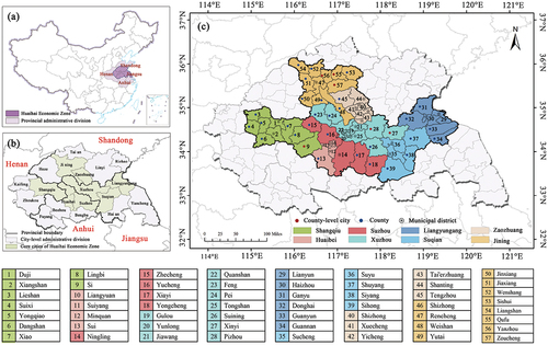
Founded in March 1986, the Huaihai Economic Zone is one of China’s first regional economic cooperation organizations. It Covers 20 prefecture-level cities in the bordering areas of four provinces: Xuzhou, Lianyungang, Suqian, Huaian, Yancheng, Jining, Heze, Linyi, Zaozhuang, Rizhao, Taian, Laiwu, Shangqiu, Kaifeng, Zhoukou, Suzhou, Huaibei, Fuyang, Bengbu and Bozhou. The total land area is 194,000 square kilometers, with a total resident population of 117 million in the region in 2021 (Shi et al. 2016). The region is located in the middle of China’s eastern coastal region, is the bridgehead of the eastern part of the Asia-Europe Continental Bridge, and has good conditions for regional development (Cai et al. 2019). However, due to many factors such as history, administrative division, and industrial structure, the Huaihai Economic Zone has developed slowly in the past thirty years, becoming an ”economic depression” between the Bohai Economic Zone and the Yangtze River Delta Economic Zone. To promote the region’s rapid economic development, the mayors of cities in the core area of the Huaihai Economic Zone held their first meeting in Xuzhou, the central city of the zone, on May 7, 2010. The meeting established the Huaihai Economic Core Area, consisting of Xuzhou, Shangqiu, Jining, Lianyungang, Zaozhuang, Suqian, Huaibei, and Suzhou. The land area is 72,400 square kilometers, and the total resident population of the region was 0.45 billion in 2021 (Urban Survey Organization of the National Bureau of Statistics 2020). The core area cities are mainly coal resource-based, and the interconnection and interaction between cities are used to drive the overall development of the whole regional economy (Zheng et al. 2022). The research object of this paper is 57 districts and counties in the core city cluster of the Huaihai Economic Zone (Figure 1).

Figure 1. 57 Districts and Counties in the Huaihai economic zone core city cluster study area. The scope of the study area follows the hierarchical relationship of provincial, city, and county levels from large to small. Figure a shows the spatial location of the Huaihai economic zone in China and its provincial relationships with the four surrounding provinces; figure b shows the extent of the city-level areas and core cities included in the Huaihai economic zone; and figure c shows the 57 county-level areas included in the core cities of the Huaihai economic zone.

2.2. Data

The predominant statistics include DMSP/OLS and NPP/VIIRS nighttime lighting, energy, socio-economic, and fundamental geographic records data.

2.2.1. Nighttime light data

DMSP/OLS nighttime lighting data was obtained from the National Oceanic and Atmospheric Administration’s National Geophysical Data Center (NOAA/NGDC) website (https://ngdc.noaa.gov/eog/dmsp/downloadV4composites.html, accessed on 2 December 2022). NPP/VIIRS data was obtained from the Colorado School of Mines (https://payneinstitute.mines.edu/eog, accessed on 14 December 2022).

2.2.2. Energy and socioeconomic data

Energy and socioeconomic data were obtained from the China Regional and China Statistical Yearbooks and city-specific statistical yearbooks.

2.2.3. Administrative divisions vector data

From 2001 to 2021, there were modifications to the administrative divisions of counties in the core city cluster of the Huaihai Economic Zone, resulting in the incorporation or withdrawal of certain counties from their authority. Thus, we chose the administrative division vector data from 2021 as the standard to exclude the impact of administrative division changes on the inconsistent statistical data standards. Information was retrieved on 3 December 2022, from (https://download.geofabrik.de/asia/china.html). Table 1 contains information on these data.

Table 1. Verification of spatial autocorrelation.

Data Name	Data Description	Source
Nighttime light	DMSP/OLS nighttime light	National Oceanic and Atmospheric Administration’s National Geophysical Data Center (NOAA/NGDC)
	NPP/VIIRS nighttime light	Colorado School of Mines
Fossil fuel combustion data	Annual total data of ten energy types, such as raw coal, coke, crude oil, gasoline, kerosene, diesel oil, fuel oil, natural gas, heat and electricity, during 2001–2021	China Statistical Yearbook, China Regional Statistical Yearbook, China Energy Statistical Yearbook and statistical yearbooks of each city
Socioeconomic data	Annual statistical data of six types, such as permanent population, GDP, per capita GDP, primary industry GDP, secondary industry GDP and tertiary industry GDP, during 2001–2021	China Statistical Yearbook, China City Statistical Yearbook, China Regional Statistical Yearbook, and statistical yearbooks of each city
Administrative boundaries	Vector files of provinces, prefectures in China	National Catalogue Service For Geographic Information
Population density	Annual data with a spatial resolution of 30 arc-seconds (approximately 1km at the equator)	OpenStreetMap (https://download.geofabrik.de/asia/china.html. accessed 3 December 2022)

3. Methodology

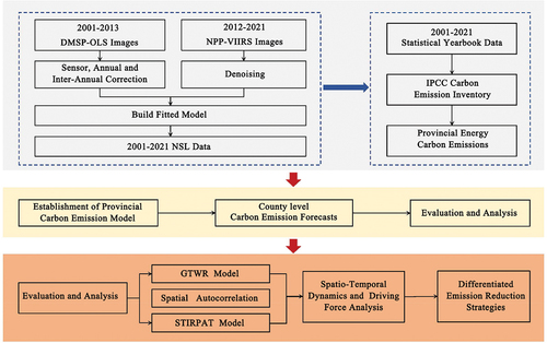
Based on nighttime light remote sensing and energy data, the spatial and temporal characteristics of carbon emissions in the core city cluster counties of the Huaihai Economic Zone from 2001 to 2021 were studied, and the influencing factors were analyzed. The overall workflow of this study is presented in Figure 2.

Figure 2. Technical roadmap.

3.1. Processing and integration of two types of night light data

3.1.1. DMSP/OLS data correction

Inter-calibration between the several OLS sensors is necessary because distinct sensors obtained the DMSP/OLS data without onboard radiometric calibration. To ensure a seamless and consistent data analysis, we employed the invariant region approach, as detailed by Wu et al. (2013), to inter-calibrate the accuracy of DMSP/OLS image data.

3.1.2. NPP/VIIRS data annual synthesis and denoising

NPP/VIIRS is better at mapping night lights than DMSP/OLS since it has a higher spatial resolution (0.5 km) and does not experience saturation. However, it leaves outliers and does not eliminate stray light, which calls for additional data cleaning. Pre-processing, including projection, cropping, and resampling, is done first, just like with the DMSP/OLS data. We resampled the data with a spatial resolution of 1 km × 1 km after converting the original geographic coordinates of WGS-1984 into Krasovsky-1940-Albers projections for 12 periods every year from 2012 to 2021.

3.1.3. Integration of two datasets using models

The coefficient of variation (cv) approach was utilized to address this issue because it is challenging to do a direct fit between the two data sets. After all, the DMSP/OLS and NPP/VIIRS data are discrete (Y. Z. Wu et al. 2022). Therefore, the 2013 DMSP/OLS and NPP/VIIRS data were utilized to calculate the cv values for all rasters with 3 km × 3 km windows. The following equation (1)(1) $\mathit{cv}=\frac{S}{x}$(1) was used to calculate the cv values:

(1) $\mathit{cv}=\frac{S}{x}$(1)

In equation (1)(1) $\mathit{cv}=\frac{S}{x}$(1) , where S and x are the standard deviation and average value of the image radiation value, respectively.

After that, the DMSP/OLS data and the NPP/VIIRS data were log-transformed to minimize the discrepancies between the two datasets and align the luminance range (Figure 3).

Figure 3. Nighttime lighting data in Huaihai economic zone core city in 2001 (a) and 2021 (b).

3.2. Energy consumption carbon-emission calculation model

Based on the energy statistics of the core cities and counties in Huaihai Economic Zone, the carbon emission coefficients of various energy sources were determined in the IPCC (2006) National Greenhouse Gas Inventory Guidelines to calculate carbon emissions, and in this study, the carbon emissions in the core cities and counties of Huaihai Economic Zone are calculated concerning Wang et al.‘s (J. Lee et al. 2015; Ouyang and Lin 2017; Y. Wang et al. 2022) calculation method and The carbon emissions are calculated using the following equation (2)(2) $\mathit{C}{O}_2=\frac{44}{12}\times \sum _{\mathit{i}=1}^{10}{K}_i{E}_i$(2) :

(2) $\mathit{C}{O}_2=\frac{44}{12}\times \sum _{\mathit{i}=1}^{10}{K}_i{E}_i$(2)

Where$\mathit{i}$is 10 energy types; $E_i$ is the consumption of energy$\mathit{i}$in terms of standard coal(10,000 tons); and$K_i$is the carbon emission factor of energy$\mathit{i}$(10,000 carbon)/(10,000 standard coal), form the default value of IPCC carbon emission calculation guidelines, where the original data unit is J. Consistent with the statistical data unit, it is converted into standard coal with a conversion factor of $1\times {10}^4$tons of standard coal equal to $2.93\times {10}^5$GJ. Carbon emission factors for various energy sources Table 2.

Table 2. Energy carbon emission factors.

Energy Type	Conversion Standard Coal Coefficient (tons of standard coal/ton)	Carbon Emission Coefficient (10^4 tons carbon/10^4 tons standard coal)
Raw Coal	0.7143	0.7559
Coke	0.9714	0.855
Crude Oil	1.4286	0.5857
Gasoline	1.4714	0.5538
Kerosene	1.4714	0.5714
Diesel	1.4751	0.5921
Fuel Oil	1.4286	0.6185
Natural Gas	1.33	0.4483
Heat	34.12	0.67
Electricity	0.345	0.272

3.3. Calculation of carbon emissions in the county

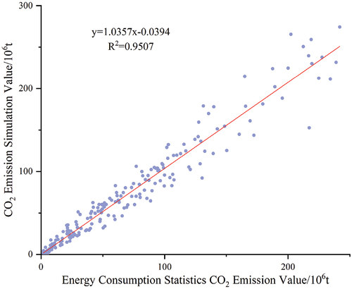
This study builds the inverse model of CO₂ emission using linear regression without intercepting, avoiding the accuracy issue brought on by smaller grid cell sizes. The findings demonstrate a very well-fitting relationship between the CO₂ statistics and the grayscale values of the night light data, suggesting that the night light data may be used to calculate CO₂ emissions in the county (Table 3).

Table 3. County carbon dioxide emissions in a linear regression model using data on evening light levels in a grayscale format.

Year	A	$R^2$	Year	A	$R^2$
2001	0.0005	0.9014	2012	0.0006	0.9402
2002	0.0006	0.9046	2013	0.0007	0.9498
2003	0.0005	0.9008	2014	0.0013	0.9526
2004	0.0007	0.9065	2015	0.0008	0.9507
2005	0.0006	0.9253	2016	0.0006	0.9524
2006	0.0005	0.9476	2017	0.0004	0.9643
2007	0.0007	0.9574	2018	0.0005	0.9265
2008	0.0006	0.9648	2019	0.0004	0.9671
2009	0.0007	0.9504	2020	0.0004	0.9687
2010	0.0005	0.9434	2021	0.0003	0.9752
2011	0.0005	0.9456

To assess the inversion model’s dependability, a correlation analysis was carried out between the estimated values of the IPCC calculation method and the inversion values of the nighttime lighting data in the core city cluster counties in the Huaihai Economic Zone from 2001 to 2021. The fitting results are shown in Figure 4.

Figure 4. Scatter plot of IPCC statistical CO₂ emission values versus fitted CO₂ emission values.

3.4. Spatio-temporal evolution

3.4.1. Geographically and temporally weighted regression (GTWR)

The Geographically and Temporally Weighted Regression (GTWR) model adds a temporal component to the classic Geographically Weighted Regression (GWR) model by considering both the temporal and spatial non-spatial dimensions. The classic Geographically Weighted Regression (GTWR) model takes account of both temporal and spatial non-stationarity and adds a temporal component (Huang, Wu, and Barry 2010). By analyzing the panel data, the GTWR model can efficiently lower the model and parameter estimate errors. In addition, it has a broader range of applications and accurately captures the variability of spatiotemporal data, enabling it to satisfy the analytical needs of complex spatiotemporal data (J. G. Liu, Li, and Ji 2021). Models are as follows:

(3) $Y_i={\beta }_0\left(u_i,v_i,t_i\right)+\sum _{\mathit{k}=1}^p{\beta }_k\left(u_i,v_i,t_i\right)X_{\mathit{ik}}+{\epsilon }_i$(3)

In equation (3)(3) $Y_i={\beta }_0\left(u_i,v_i,t_i\right)+\sum _{\mathit{k}=1}^p{\beta }_k\left(u_i,v_i,t_i\right)X_{\mathit{ik}}+{\epsilon }_i$(3) ,$Y_i$is the explanatory variable for the i-th sample region.$X_{\mathit{ik}}$is the observed value of the k-th explanatory variable in the i-th sample region. ($u_i$, $t_i$) are the spatiotemporal coordinates of the i-th sample region.${\beta }_0$($u_i$, $t_i$) is the spatiotemporal intercept of the i-th sample region.${\beta }_k$($u_i$, $v_i$, $t_i$) is the regression coefficient for the k-th explanatory variable at the i-th sample region.$\mathit{\beta }$ > 0 indicates that the explanatory variables are positively correlated with the explained variables and vice versa,${\epsilon }_i$is the random disturbance term. This paper implements the GTWR model mainly using ArcGIS10.6 software and the GTWR plug-in made by Huang et al. The bandwidth is optimally set using AICc, and the ratio of spatiotemporal distance parameters is 1.

3.4.2. Spatial autocorrelation

Spatial autocorrelation is a technique for analyzing spatial data that can be used to estimate and analyze the degree of spatial dependency between study areas. It can also highlight the spatial heterogeneity and spatial dependability of geographic data. Spatial autocorrelation can be further classified into two categories: local and global (X. X. Wang, He, and Zhao 2020). This article uses this approach to examine the spatial dependency pattern of carbon emissions in the counties that make up the Huaihai Economic Zone’s core urban agglomeration.

3.4.2.1. Global spatial autocorrelation

By computing Moran’s I index’s values, scores, and scores, global spatial autocorrelation was utilized to evaluate the index’s importance. The following is the formula:

(4) $\mathit{I}=\frac{\mathit{n}\sum _{\mathit{i}=1}^n\sum _{\mathit{j}=1}^n{W}_{\mathit{ij}}\left(X_i-\bar{X}\right)\left(X_j-\bar{X}\right)}{\sum _{\mathit{i}=1}^n\sum _{\mathit{j}=1}^n{W}_{\mathit{ij}}\sum _{\mathit{i}=1}^n{\left(X_i-\bar{X}\right)}^2}$(4)

In equation (4)(4) $\mathit{I}=\frac{\mathit{n}\sum _{\mathit{i}=1}^n\sum _{\mathit{j}=1}^n{W}_{\mathit{ij}}\left(X_i-\bar{X}\right)\left(X_j-\bar{X}\right)}{\sum _{\mathit{i}=1}^n\sum _{\mathit{j}=1}^n{W}_{\mathit{ij}}\sum _{\mathit{i}=1}^n{\left(X_i-\bar{X}\right)}^2}$(4) ,$\mathit{n}$ is the total number of units in the districts and counties;$X_i$and$X_j$are the carbon emissions for region$\mathit{i}$and region$\mathit{j}$respectively;$\mathit{X}$ is the average of carbon emissions from all regions;$W_{\mathit{ij}}$is the spatial weight matrix, which is obtained based on the Rook neighbor relationship. Moran’s I values range between -1 and 1. Values closer to 1 indicate a stronger positive correlation, while values closer to -1 indicate a stronger negative correlation. Values close to 0 indicate a lack of significant correlation. The significance of the global Moran’s I index can be tested by the size of the Z-value (Table 4).

Table 4. Spatial autocorrelation verification.

$\mathit{Z}$Score	$\mathit{P}$Value	Spatial Autocorrelation
$\mathit{Z}$≤ 1.96	$\mathit{P}$> 0.05	Non-existent
$\mathit{Z}$≥ 1.96	$\mathit{P}$< 0.05	Exist
$\mathit{Z}$≥ 2.58	$\mathit{P}$< 0.01	Extremely strong

3.4.2.2. Local spatial autocorrelation

For spatial clustering analysis, the local Moran’s I index serves as a local indication of spatial autocorrelation. The following is the formula:

(5) $I_i=Z_i\sum _j{W}_{\mathit{ij}}{Z}_j$(5)

In equation (5)(5) $I_i=Z_i\sum _j{W}_{\mathit{ij}}{Z}_j$(5) ,$I_i$is the local Moran’s I index;$Z_i$and$Z_j$are spatial units and standardized carbon emissions;$W_{\mathit{ij}}$is the spatial weight matrix. The carbon emissions in the study area were classified according to the local Moran’s I index as follows: high-high (H-H), low-low (L-L), low-high (L-H), high-low (H-L), and insignificant. In which H-H and L-L indicate that the adjacent regions have a spatially positive correlation, H-H represents that the adjacent regions are all high carbon emission regions, and L-L represents that the adjacent regions are all low carbon emission regions; L-H and H-L indicate that high carbon emission regions surround low carbon emission regions and high carbon emission regions are surrounded by low carbon emission regions, respectively.

3.5. Influencing factors

American demographers Ehrlich and Holdren created the IPAT (Impact, Population, Affluence, Technology) model 1971 (Ehrlich and Holdren 1971). It eliminates the impact of the same proportionate change problem and looks at the specific effects of wealth, population, and technology variables on the environment as they change. The following is the model:

(6) $\mathit{I}=\mathit{P}\times \mathit{A}\times \mathit{T}$(6)

In equation (6)(6) $\mathit{I}=\mathit{P}\times \mathit{A}\times \mathit{T}$(6) , I denotes the environmental impact. P denotes the size of the population. A denotes affluence.

By putting out a stochastic regression impact model called STRIPAT (Stochastic Impacts via Regression on Population, Affluence, and Technology), Dietz et al. improved upon the conventional IPAT. Because of its versatility, this model is frequently employed in many different sectors. In order to investigate the determinants of CO₂ emissions further, the STIRPAT model can better reflect regional environmental pressures through carbon emissions from energy consumption. The following is the model:

(7) $I_i=\mathit{a}\times P_i^b\times A_i^c\times T_i^d\times e_i$(7)

In equation (7)(7) $I_i=\mathit{a}\times P_i^b\times A_i^c\times T_i^d\times e_i$(7) , $\mathit{a}$represents the model coefficients.$\mathit{b}$,$\mathit{c}$,$\mathit{d}$ represents the impact factor index. I, P, A, and T are environmental pressure, population size, affluence, and technology level, respectively;$\mathit{e}$is the model error term. The advantage of the STIRPAT model is that the coefficients can be estimated as parameters, and each influencing factor can be decomposed appropriately. Based on existing research results, the STIRPAT model is extended to consider that factors such as urbanization level and industrial structure also impact carbon emissions (Xue et al. 2023). Therefore, such factors are incorporated into the model separately and logarithmically for both sides of the equation, which is expressed as follows:

(8) $\mathit{In}{\left(\mathit{CI}\right)}_t=\mathit{In\alpha }+{\beta }_1\mathit{InP}+{\beta }_2\mathit{InD}+{\beta }_3\mathit{InG}+{\beta }_4\mathit{InS}+{\beta }_5\mathit{InU}+{\beta }_6\mathit{InE}+\mathit{In}{\epsilon }_t$(8)

In equation (8)(8) $\mathit{In}{\left(\mathit{CI}\right)}_t=\mathit{In\alpha }+{\beta }_1\mathit{InP}+{\beta }_2\mathit{InD}+{\beta }_3\mathit{InG}+{\beta }_4\mathit{InS}+{\beta }_5\mathit{InU}+{\beta }_6\mathit{InE}+\mathit{In}{\epsilon }_t$(8) , CI is the environmental quality factor (regional carbon emissions),$\mathit{a}$is a constant term, P denotes population size, D denotes population density, G denotes the economic size, S denotes industrial structure, U denotes urbanization level, and E denotes technological progress. ${\beta }_1-{\beta }_6$ is the elasticity coefficient of the corresponding variable. That is, when each 1% change in P, D, G, S, U, and E causes changes in${\beta }_1\mathrm{\%}$,${\beta }_2\mathrm{\%}$,${\beta }_3\mathrm{\%}$,${\beta }_4\mathrm{\%}$,${\beta }_5\mathrm{\%}$, and${\beta }_6\mathrm{\%}$, respectively, InƐ_t of CI is the model random error term, which indicates other factors affecting environmental quality (Table 5, Table 6).

Table 5. Definition of carbon emission impact factors indicators.

Variable Dimension		Abbreviations	Explanatory variables	Unit
F1	Population size	POP	Total household population by county	million people
F2	Density of Population	DOP	Number of people per unit of land area	People /km^2
F3	Gross Domestic Product	GDP	Gross regional product by county	million RMB
F4	Per capita GDP	PGDP	GDP per capita	million RMB
F5	Industrial Structure	SIND	The scale of output value of secondary industry	million RMB
F6	Urbanization level	UR	Non-agricultural population as a proportion of the total regional population	%
F7	Energy consumption per unit GDP	EI	Energy consumption per unit of GDP	Tons/RMB

Table 6. Statistical description of relevant variables.

Variables	F1	F2	F3	F4	F5	F6	F7
Mean value	83.78	907.92	155.57	2.03	44.167	36.48	2.92
Standard deviation	45.33	1090.54	179.78	1.04	11.66	23.63	2.09
Minimum value	13.14	255.47	8.27	0.26	9.97	6.46	0.26
Maximum Value	439.87	8299.83	1085.37	2.03	81.64	99.98	14.53

4. Results

4.1. Characteristics of the overall pattern of carbon emissions

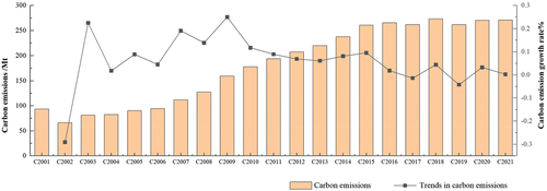
From 2001 to 2021, the overall carbon emissions of the Huaihai economic core cities and counties showed a trend of “rapid and then slow” continuous growth (Figure 5), and the total carbon emissions increased from 63.4.2 Mt to 279.89 Mt, with an overall growth rate of 341.32% and an average annual growth rate of 7.92%. In particular, the growth rate was faster from 2004 to 2009, with an average annual growth rate of 14.04%, and entered a steady growth phase from 2010 to 2015, with an average annual growth rate of 7.71%. The specific targets of energy conservation and emission reduction in “The Thirteenth Five-Year Plan” provided strong policy constraints to eliminate backward production capacity and promote the upgrading of polluting enterprises, which slowed down the growth rate of total carbon emissions in the counties after 2015 and fell back in 2019, with an average growth rate of 0.65% from 2015 to 2021. Therefore, to better compare and analyze the spatial and temporal evolution and influencing factors of carbon emissions in the region, six-time points in 2001, 2005, 2009, 2013, 2017, and 2021 were selected according to the characteristics of different carbon emission stages as crucial analysis points.

Figure 5. Trends of total carbon emissions in core cities and counties of the Huaihai economic zone, 2001–2021.

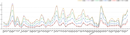
Statistical analysis of carbon emission changes in each district and county from 2001 to 2021 reveals the variability among regions (Figure 6). In 2001, the county with the highest carbon emissions was Tengzhou County-level City (4.49 Mt), followed by Zoucheng County-level City (3.78 Mt), Tongshan Municipal District (3.44 Mt), Yongqiao Municipal District (3.33 Mt), and Rencheng Municipal District (2.69 Mt), In 2021, the areas with high carbon emissions were Yongqiao Municipal District (9.93 Mt), Tongshan Municipal District (9.65 Mt), Tengzhou County-level City (9.42 Mt), Pizhou County-level City (8.61Mt) and Donghai County (8.29Mt). During the study period, Tengzhou County-level City, Yongqiao Municipal District, Tongshan Municipal District, Zoucheng County-level City, Rencheng Municipal District, Donghai County, Muyang County, Pizhou County-level City, Ganyu County, and Yanzhou Municipal District have been high carbon emission areas, maintaining a proportion of about 30% of the total carbon emissions of the 57 counties in all years. This is because these areas are rich in coal and petrochemical energy resources, belong to the traditional energy extraction and consumption sectors, and have a high proportion of secondary industry in their industrial structures. Additionally, after the government lifted restrictions following the 2020 COVID-19 epidemic in April, there was an increase in energy consumption. The regional economic development and a high degree of reliance on carbon-intensive, high-polluting enterprises resulted in total carbon emissions remaining high.

Figure 6. Changes in carbon emissions by district and counties,2001–2021.

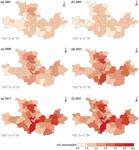
To better analyze the spatial and temporal evolution of carbon emissions from 2001 to 2021, ArcGIS 10.6 software was used to visualize the carbon emissions in the counties of the Huaihai Economic Zone core city cluster. Spatial distribution maps of carbon emissions in these counties for 2001, 2005, 2009, 2013, 2017, and 2021 were obtained (Figure 7). Regarding the temporal pattern, the total carbon emissions of all counties and districts were less than 5.5 Mt during 2001–2008. Three districts and counties had total carbon emissions more significant than 5.5 Mt in 2009, and ten districts and counties exceeded 5.5 Mt in 2013, with three of them above 7.5 Mt. The number of high carbon emission areas (≥7.5 Mt) increased to seven in 2017, showing a significant expansion trend. After 2017, the carbon emissions of each district and county became more stable, and some districts and counties reduced their carbon emissions. In terms of the spatial pattern, the high carbon emission area (≥7.5Mt) is mainly concentrated in the central counties, and the low carbon emission area (≤3.5Mt) is mainly concentrated in the eastern and western counties. The current spatial distribution pattern of carbon emissions is high in the middle and low in the east and west, with the “core-edge” structure of carbon emissions becoming increasingly prominent.

Figure 7. (a) State of carbon emission in the Huaihai economic zone in 2001, (b) state of carbon emission in the Huaihai economic zone in 2005, (c) state of carbon emission in the Huaihai economic zone in 2009, (d) state of carbon emission in the Huaihai economic zone in 2013, (e) state of carbon emission in the Huaihai economic zone in 2017, (f) state of carbon emission in the Huaihai economic zone in 2021; spatial and temporal changes in carbon emissions 2001–2021.

4.2. Spatial autocorrelation analysis of carbon emissions

By calculating the global Moran’s I index of total carbon emissions in the core cities of the Huaihai Economic Zone counties from 2001 to 2021, the aim is to analyze the degree of spatial agglomeration of carbon emissions (Table 7). The global Moran’s I index values of all years are positive, and all of them pass the significance level test of 0.01, indicating that the carbon emissions of neighboring counties have a significant positive spatial correlation, showing a significant clustering phenomenon. Districts and counties with higher carbon emissions are adjacent, and those with lower carbon emissions are also adjacent. The global Moran’s I index shows a wavy downward trend regarding time patterns. It decreased from 0.5235 in 2001 to 0.3921 in 2007 and gradually increased to 0.4547 in 2012. The economic crisis that occurred in the same year caused the GDP, PGDP, and SIND to be hit, prompting the Moran’s I index to fluctuate more, and the overall gradually decreased over time, and by 2021 Moran’s I decreased to 0.3914. This result indicates that the degree of spatial agglomeration of carbon emissions (including H-H agglomeration and L-L agglomeration) among counties in the Huaihai economic core area gradually decreases. With the socio-economic development of the Huaihai Economic Core City Group, the carbon emissions of each district and county have increased significantly, mainly due to the industrial transformation of the eastern counties and the main urban areas, the construction of ecological civilization, and the implementation of the green development concept. These factors have promoted narrowing the carbon emission gap between counties and their gradual spatial convergence.

Table 7. Global Moran’s I of CO₂ emissions at the county level, 2001– 2021.

Year	Global Moran’s I	Z Score	P Value
2001	0.5235	4.8508	0.001
2002	0.5264	5.1121	0.001
2003	0.4206	4.0567	0.001
2004	0.4632	4.3368	0.001
2005	0.4065	4.1276	0.001
2006	0.3955	3.8757	0.003
2007	0.3921	3.7671	0.002
2008	0.4018	3.9795	0.001
2009	0.4555	4.3931	0.001
2010	0.4422	4.2318	0.001
2011	0.4522	4.3683	0.001
2012	0.4547	4.3911	0.001
2013	0.4451	4.3295	0.001
2014	0.4366	4.0091	0.001
2015	0.4155	3.8521	0.001
2016	0.4116	3.9886	0.001
2017	0.4061	4.0993	0.001
2018	0.4063	4.2453	0.001
2019	0.4065	4.1419	0.001
2020	0.4016	4.0977	0.001
2021	0.3914	3.8957	0.002

The global Moran’s I index can only judge and identify the regional variability of county-scale carbon emissions in the core cities of the Huaihai Economic Zone. However, it still cannot reveal the spatial agglomeration characteristics of their internal carbon emissions. Therefore, local spatial autocorrelation analysis was conducted for carbon emissions in six necessary time cross-sections: 2001, 2005, 2009, 2013, 2017, and 2021 (Figures 8–9).

Figure 8. Spatial autocorrelation local clustering analysis of carbon emissions. (a) Carbon emission local cluster analysis, 2001. (b) Carbon emission local cluster analysis, 2005. (c) Carbon emission local cluster analysis, 2009. (d) Carbon emission local cluster analysis, 2013. (e) Carbon emission local cluster analysis, 2017. (f) Carbon emission local cluster analysis, 2021.

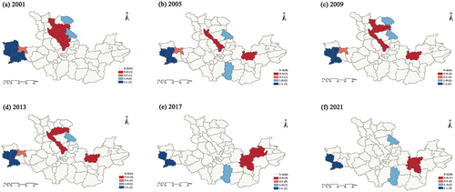
Figure 9. Spatial autocorrelation local significance analysis of carbon emissions. (a) Carbon emission local significance analysis, 2001. (b) Carbon emission local significance analysis, 2005. (c) Carbon emission local significance analysis, 2009. (d) Carbon emission local significance Analysis, 2013. (e) Carbon emission local significance analysis, 2017. (b) Carbon emission local significance analysis, 2021.

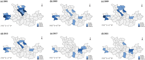
Overall, the spatial agglomeration effect of carbon emissions in the Huaihai Economic Core City Group counties is more evident. H-H agglomeration and L-L agglomeration are the main types of local spatial autocorrelation. The number of counties with H-H agglomeration increases significantly, while the number of counties with L-L agglomeration decreases gradually, showing a more distinct stratified agglomeration phenomenon. The center of gravity of the distribution of H-H agglomeration counties gradually shifted from the northwest to the southeast during the study period. The H-H agglomerations initially found in Yanzhou Municipal District, Qufu County-level City, Zoucheng County-level City, Tengzhou County-level City, Xuecheng Municipal District, and Weishan County in 2001 gradually disappeared and shifted to Donghai County, Xinyi County-level City, and Suyu Municipal District after 2017. Additionally, the L-L agglomeration area included Sui County, Zhecheng County, Ningling County, Minquan County, and Suiyang Municipal District in 2001, but by 2021, only Zhecheng County remained. This change is mainly due to Zhecheng County being dominated by primary industries with fewer carbon-intensive manufacturing industries, resulting in lower carbon emissions. The energy consumption level of Xinyi County-level City has improved considerably with urban development. However, insufficient energy utilization and carbon reduction technologies make overcoming the bottleneck of path dependence in carbon emission levels over a certain period challenging.

4.3. Analysis of carbon emission influencing factors

The results of the previous study indicated an uneven spatial and temporal distribution of carbon emissions in the Huaihai economic core city cluster, and carbon emissions exhibit spatial and temporal non-smoothness. Due to each variable’s varying degrees of influence on different carbon emissions, the spatial and temporal heterogeneity of carbon emission intensity in the counties of the Huaihai Economic Core City Group needs to be explored locally. Based on the panel data of each county in the Huaihai Economic Core City Cluster from 2001–2021, carbon emissions in each county and region are used as the explanatory variables, while F1 (POP), F2 (DOP), F3 (GDP), F4 (PGDP), F5 (SIND), F6 (UR), and F7 (EI) are used as explanatory variables. Geographically and Temporally Weighted Regression (GTWR) estimates the parameters of carbon emission influencing factors for different periods in the study area.

4.3.1. GTWR model construction and analysis of empirical results

The correlation analysis (Table 8) was conducted for each explanatory variable using SPSS 22.0 software. The variance inflation factor (VIF) of each explanatory variable was within 10, the tolerance was greater than 0.1, and there was no obvious multiple covariance effect, so regression analysis could be conducted (García et al. 2015).

Table 8. Multi-collinearity test.

Variables	F1	F2	F3	F4	F5	F6	F7
Tolerance	0.508	0.658	0.415	0.554	0.859	0.505	0.537
VIF	1.969	1.519	2.409	1.806	1.165	1.979	1.864

Using the GTWR model, the goodness-of-fit R² and AICc were selected as the evaluation indicators of the model’s confidence, and the parameter estimation results were analyzed (Table 9). The GTWR model can more accurately analyze the spatial and temporal heterogeneity of each influencing factor on the carbon emissions in the counties of the Huaihai Economic Core City Cluster in the time dimension and spatial dimensions.

Table 9. Comparison of model evaluation indexes.

Variables	OLS	GTWR
AIC	1032.01	802.383
R^2	0.7122	0.9346
Adjustment of R^2	0.7014	0.9332
AIC change amount	0	229.627
R^2 change amount	0	0.2224

Based on the county panel data of the Huaihai economic core city cluster from 2001 to 2021, the GTWR model was used to estimate the parameters of the influencing factors of carbon emissions in each county at different times to explore the spatial and temporal heterogeneity of the influence of each factor on carbon emissions in the study region. The results of descriptive statistics are shown in Table 10. As shown in Table 9, the regression coefficients of total Population Size (POP), Density of Population (DOP), Gross Domestic Product (GDP), Per capita GDP (PGDP), Industrial Structure (SIND), Urbanization on Level (UR), and Energy consumption per unit GDP (EI) exhibit significant variation. This indicates substantial differences in the influencing factors of carbon emissions in each county, highlighting the need to consider local carbon emissions’ spatial and temporal heterogeneity.

Table 10. Descriptive statistics of regression coefficients of the GTWR model.

Variables		Minimum	Maximum	Average	Median	Standard deviation
F1	POP	−0.0136	1.7414	0.7193	0.3742	0.6577
F2	DOP	−0.6713	0.4024	−0.0428	0.0135	0.1749
F3	GDP	0.2149	7.3182	3.0153	3.3582	2.4939
F4	PGDP	−0.2165	0.9589	0.3298	0.2704	0.3054
F5	SIND	−0.1320	−0.5325	0.0951	0.0129	0.1944
F6	UR	−0.2410	0.5267	0.0059	−0.0771	0.1951
F7	EI	0.4675	2.6747	0.8681	0.7068	0.4614

4.3.2. Time evolution of each influencing factor

The regression analysis of carbon emission influencing factors in the Huaihai economic core cities and counties at different times was carried out using the GTWR model to obtain the contribution coefficients of each influencing factor to carbon emissions at different spatial and temporal locations. A box plot of each coefficient over time was then drawn to clarify the evolution trend of each factor over time. The contribution of F1 (POP) to carbon emissions is more significant (Figure 10), showing a positive effect from population size in most counties within the Huaihai economic core urban agglomeration, with only a few counties having negative regression coefficients. As the population increases, carbon emissions also increase. The regression coefficient of population size tends to increase and then decrease over time, with the dispersion first decreasing and then gradually increasing. The decreasing trend may be because the counties and regions are constantly optimizing their economic structure and improving the comprehensive utilization of energy and resources to control the increase in carbon emissions. The increasing dispersion is due to differences in economic development and population size between different regions, leading to significant differences in carbon emissions.

Figure 10. Time series change trend of GTWR regression coefficients. (a) F1 (POP) time series trends of regression coefficients, 2001–2021; (b) F2 (DOP) time series trends of regression coefficients, 2001–2021; (c) F3(GOP)Time series trends of regression coefficients, 2001–2021; (d) F4(PGOP) time series trends of regression coefficients, 2001–2021; (e) F5 (SIJND) time series trends of regression coefficients, 2001–2021; (f) F6(UR)time series trends of regression coefficients, 2001–2021; (g) F7(UR)Time series trends of regression coefficients, 2001–2021.

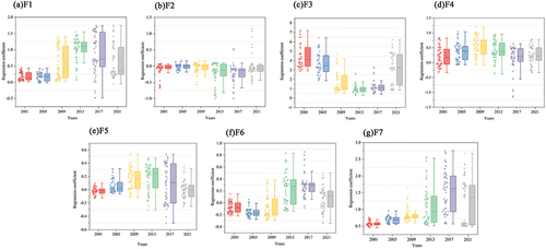
The regression coefficient of F2 (DOP) is negative (Figure 10), indicating that population agglomeration suppresses carbon emissions. Population concentration leads to the spatial clustering of economic activities and production factors, resulting in changes in energy use and transportation patterns (C. Li, H. Li, and X. H. Qin 2022). This reduces marginal abatement costs through the scale effect (Shen, Zhao, and Wang 2002), facilitates the effective allocation and intensive use of energy resources (J. S. Fan and Zhou 2019), allows for centralized supervision by government departments, and reduces the county’s carbon emissions level.

F3(GDP) economic size makes the most significant contribution to carbon emissions, and the regression coefficients are positive for all counties during the study period (Figure 10). There is a U-shaped relationship between economic scale and carbon emissions in the Huaihai Economic Core City Group counties. The counties in the study area are all deeply inland, most are still at the primary stage of development, and the lack of economic development drives each county’s high carbon spillover effect. Disadvantages in location, talent, technology, and infrastructure contribute to a vicious circle of poverty. In the future, the economic scale will more obviously promote carbon emissions.

The regression coefficient for F4(PGDP) was essentially positive (Figure 10). PGDP is an essential indicator of the affluence of a country’s inhabitants, and the impact on carbon emissions is mainly manifested in the growth of the economic level, leading to an increase in the consumption structure and per capita consumption level of the inhabitants. Consumer goods indirectly carry the carbon emissions generated by energy consumption. It can be seen that the growth of wealth stimulates people’s desire to consume, and the growth of consumption drives energy demand, which directly contributes to carbon emissions.

The regression coefficient of F5(SIND) shows a trend of increasing and decreasing (Figure 10). Most counties within the Huaihai economic core urban agglomeration suffer from strong resource dependence, inefficient industrial development, and inefficient energy consumption. High emissions and high pollution place the initially fragile ecological background under heavier ecological and environmental pressure. Since the “Twelfth Five-Year Plan” and “Thirteenth Five-Year Plan” put forward the goals of optimizing and adjusting the economic structure, promoting low-carbon economic development, and improving the construction of ecological civilization, the counties and districts have made adjustments to their industrial structures and controlled their carbon emissions.

The regression coefficient of F6 (UR) showed a negative to positive change during the study period (Figure 10). In the early stage of the study, the increase in urbanization level had some inhibiting effect on carbon emissions due to the deployment and implementation of the urbanization development strategy. However, with the continuous urbanization process, the regression coefficient began to rebound in 2013. This was due to the population boom in the county and the expanding demand for energy resource consumption, resulting in a continuous rise in carbon emissions. The introduction of National New Town Planning in 2014 made urbanization enter a new stage, emphasizing a people-oriented approach and promoting social life and consumption with green and low-carbon concepts. Consequently, the regression coefficient of urbanization level began to decrease, eventually reducing carbon emissions.

The contribution of F7(EI) to carbon emissions is positive and shows a decreasing trend after 2018 (Figure 10). On the one hand, technological progress improves energy use efficiency through low-carbon production technologies, reducing energy consumption and pollution emissions per unit of GDP. However, there is also an increase in energy consumption and carbon emissions due to lower unit consumption costs. On the other hand, as urbanization accelerates, the industrial structure is transformed and upgraded, with the focus of development gradually shifting from industry to modern service and high-tech industries. This shift largely contributes to the reduction of energy intensity.

4.3.3. Spatial heterogeneity of factors influencing carbon emissions

To more intuitively explore the variability of the influence of different factors on carbon emissions in each county and region, the regression results based on the GTWR model were visualized using ArcGIS 10.6 to generate spatial and temporal distribution maps of the regression coefficients of the influencing factors.

The F1 (POP) regression coefficient ranges from −0.0136 to 1.7414, indicating a wide span (Figure 11). The counties significantly influencing population size include Zoucheng County-level City, Tengzhou County-level City, Jinxiang County, Feng County, Liangyuan Municipal District, Yucheng County, Guanyun County, and Guannan County.

Figure 11. Spatial distribution patterns of carbon emission influencing factors based on GTWR model. (a) F1(POP)Spatial distribution characteristics of county territory. (b) F2(DOP)Spatial distribution characteristics of county territory. (c) F3(GOP)Spatial distribution characteristics of county territory. (d) F4 (Pgop)spatial distribution characteristics of county territory. (e) F5(SIJND)Spatial distribution characteristics of county territory. (f) F6(UR)Spatial distribution characteristics of county territory. (g) F7(EI) spatial distribution characteristics of county territory.

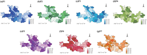
The regression coefficient of F2 (DOP) for population agglomeration and carbon emissions does not fluctuate much (Figure 11). The area most influenced by population agglomeration is Xiao County, while the areas less influenced are mainly concentrated in the south of the study area, primarily Suining County, Lingbi County, and Yongqiao Municipal District.

The regression coefficients of F3 (GDP) for economic scale are all positive (Figure 11). Xuecheng Municipal District has the largest regression coefficient, followed by Fengcheng Municipal District, Ganyu Municipal District, and Haizhou Municipal District. The coefficients in this interval range from 6.2434 to 7.3182. In the process of promoting economic development, these areas have been expanding construction land and developing heavy industries, which increase energy demand and lead to excessive increases in carbon emissions. The lowest values of the regression coefficient are relatively concentrated in counties focused on primary industry, such as Dangshan County and Xiayi County. These regression coefficients range from 0.2149 to 0.4569.

The regression coefficients of F4 (PGDP) ranged from -0.2165 to 0.9589 (Figure 11). The regression coefficients of Tongshan Municipal District, Sihong County, Guanyun County, Qufu County-level City, Zhecheng County, Lieshan Municipal District, and Yuntai Municipal District were between 0.6402 and 0.9589, while those of Wenshang County, Rencheng Municipal District, Minquan County, Taierzhuang Municipal District, Suyu County, and Haizhou Municipal District were between -0.2165 and -0.0392.

The F5 (SIND) regression coefficients did not show consistent positive or negative correlations (Figure 11). The areas affected by a higher industrial structure are mainly in counties such as Zoucheng County-level City, Tengzhou County-level City, Feng County, and Yucheng County. These areas are characterized by heavy industries, rich in coal and metal resources, and a higher share of secondary industries, leading to increased carbon emissions.

The F6(UR) regression coefficients are distributed positively and negatively from −0.2411 to −0.5267 (Figure 11), with higher influence observed in the western region and lower influence in the eastern region. The counties and regions most affected by urbanization levels are Liangyuan Municipal District, Yucheng County, Suixian County, Jinxiang County, and Zoucheng County-level City. Quanshan Municipal District and the Pizhou County-level City of Xuzhou have been designated as pilot areas for the low-carbon transformation of old industrial cities, actively promoting the optimization and upgrading of energy and industrial structures and strengthening the capacity for energy conservation and emission reduction through science and technology innovation, which can effectively control carbon emissions.

The F7(EI) technological progress regression coefficients were positive (Figure 11). Lianyun Municipal District has the most significant degree of influence on carbon emissions in the region, followed by Pei County, Gulou Municipal District, Jiaxiang County, Shizhong Municipal District, Suiyang County, Sucheng Municipal District, Xiaoxian County, and Xiayi County.

5. Discussion

5.1. Spatial and temporal evolution of county carbon emissions and policy development

The results of this study on carbon emissions in the core cities and counties of the Huaihai Economic Zone are relatively similar to those of scholars such as Y. Chen and Rajakani (2022), K. Shi et al. (2016), and H. Chen et al. (2020). The three stages of sluggish development in the early stage, rapid growth in the middle stage, and slow growth in the late stage are evident in the growth rate of carbon emissions throughout this time, which is in line with the findings of H. Meng et al. (2023) and others. Trends in carbon emissions throughout the study period are closely linked to policy developments. The implementation of policies to accelerate urban economic development, industrial upgrading, and transfer, as well as promote the development of urban and rural areas is primarily reflected in “The Tenth Five-Year Plan” and “The Eleventh Five-Year Plan.” This results in the highest average annual carbon emissions of 14.04% during the same period, which is concentrated in resource-type counties such as Yanzhou Municipal District and Tongshan Municipal District, consistent with the study’s findings by Song et al. (2022). The State Council released “The Thirteenth Five-Year Plan” in 2016 to reduce greenhouse gas emissions. The plan said there has been a discernible decline in carbon emissions due to changes in energy consumption practices and the manufacturing sector’s transformation (Yang et al. 2020; Zhu et al. 2019). Population movement and agglomeration impact lifestyles, consumption patterns, and the demand for energy in terms of geographical distribution and agglomeration. These factors ultimately result in a rise in CO₂ emissions (D. Zhang et al. 2021). 2021 Yongqiao Municipal District, Tongshan Municipal District, and Tengzhou County-level City will emit the most significant carbon emissions of 9.93 Mt, 9.65 Mt, and 9.42 Mt, respectively. Consequently, the built-up region will continue to be a crucial location for carbon emission reduction strategies in the future, which will result in a drop in CO₂ emissions. Contribute favorably to the county’s efforts to reduce carbon emissions.

China’s economy contracted 6.8% in the first quarter of 2020 due to government controls implemented following the COVID-19 outbreak (National Bureau of Statistics 2020). Carbon emissions fell by 11.5% from January to April compared to the same period in 2019 (B. Zheng et al. 2020). After lifting restrictions in April, a timely resumption of work was carried out, particularly in the core cities of the Huaihai Economic Zone, where the county-level resumption rate was higher. The increase in industry, energy consumption, and investment led to a rebound in carbon emissions in the region (Guan et al. 2020). The region’s high share of secondary industries, predominantly coal-related, raised the overall carbon emissions (Sun and Mi 2023), resulting in the total for 2020 exceeding that of 2019. This situation persists into 2021, with Yongqiao Municipal District, Tongshan Municipal District, and Tengzhou County-level City emitting the most significant carbon emissions at 9.93 Mt, 9.65 Mt, and 9.42 Mt, respectively. Consequently, the built-up region will continue to be a crucial location for carbon emission reduction strategies in the future, contributing favorably to the county’s efforts to reduce carbon emissions.

5.2. Role of county carbon emission influencing factors

Research on the influencing factors of carbon emissions is the basis for assessing environmental impacts, defining emission reduction paths, and setting emission reduction targets. This study empirically analyzes the regional differences of carbon emissions in the core cities and counties of the Huaihai Economic Zone, visualizes the coefficients of influencing factors such as POP, DOP, GDP, PGDP, SIND, UR, and EI using the GTWR model, and reveals the regional heterogeneity of carbon emissions by revealing the influence of different factors on carbon emission results from a spatial and temporal perspective. The results show that the model has good stability and fitting effect (Table 7, Figure 10). This research is distinct from previous findings; Chen et al., for instance, identify three important control variables for China’s province’s carbon emissions (D. Zhang et al. 2021), but they do not examine the contributing variables. Although Song et al. (2022) examined the factors influencing carbon emissions, their examination of particular causes was limited to elements like industrial structure and urbanization, ignoring environmental considerations and technological advancements. By considering them, this study contributes to understanding how county-level carbon emissions are influenced. The accuracy and stability of the results will decline when the pertinent elements are incorporated into the model for analysis (C. Li, Li, and Qin 2022).

According to the study, economic status is the primary factor influencing carbon emissions, which is in line with Wang’s results (Z. Wang et al. 2012). Since 2005, the Huaihai Economic Zone’s core cities and counties’ carbon emission curves have positively correlated with the economic development curve. This is because an energy-based economic development model, coupled with rapid economic growth, has increased CO₂ emissions (Zhao, Sun, and Qin 2022). In the future economic growth of countries with larger GDPs, energy efficiency should be increased, and sophisticated technology should be embraced (J. W. Lee 2013). Nonetheless, further debate is necessary about selecting influencing elements, as several academics have selected various factors (Guo et al. 2022; Z. S. Meng, Wang, and Wang 2018; Tong, Tong, and Li 2016), each of which has a varied impact on the results. Despite the relative complexity of the components influencing carbon emissions, the STIRPAT model is highly scalable (D. N. Liu and Xiao 2018; Q. Wang et al. 2022). Consequently, this study does not include all impact factor indicators; it selects impact factors based on the accessibility of municipal statistics yearbook data. Research findings about carbon emissions will be more accurate if the statistical index system of data at various study area scales is developed and enhanced. Additionally, the perspective of smaller study area sizes can break down the intricate interactions between many factors, which is the path that future research on carbon emissions will take.

6. Conclusions

This paper presents a comprehensive research framework with 57 counties in the core cities of the Huaihai Economic Zone. It analyzes the evolution and heterogeneity of county carbon emissions’ spatial and temporal patterns and driving influences from 2001 to 2021 by combining the GTWR model, spatial autocorrelation, and STIRPAT model. The conclusions are as follows.

1. In the temporal evolution, the carbon emissions of the Huaihai economic core urban agglomeration from 2001 to 2021 all experienced three phases, with the rapid growth phase occurring from 2005 to 2015, when the average annual growth rate of carbon emissions reached 10.86% and there was a significant expansion trend of high carbon emission counties. After 2015, the carbon emissions of each district and county are more stable, with an average annual growth rate of only 0.65% and a steady decrease in carbon emissions.

2. In the spatial evolution, the overall distribution pattern of carbon emissions in the region’s counties is high in the middle and low in the east and west, according to the spatial correlation analysis. The coefficient of variation of carbon emissions and the global Moran’s I index of each county and district within the Huaihai Economic Core City Cluster show a decreasing trend to 0.3914 from 2001 to 2021, indicating that the spatial variation and agglomeration of carbon emissions gradually decreased. The counties in the Huaihai Economic Core City Group show a more apparent stratified agglomeration phenomenon in the spatial pattern as a whole, and the counties have a high spatial dependence pattern of carbon emissions on a local scale. Most counties with high (low) carbon emissions are adjacent to those with high (low) carbon emissions. In addition, Tengzhou County-level City, Yongqiao Municipal District, Tongshan Municipal District, and Zoucheng County-level City have a “high carbon lock” effect, so these districts and counties need to take carbon reduction measures as soon as possible to get rid of the carbon lock phenomenon gradually.

3. There is significant spatial and temporal heterogeneity in the factors influencing carbon emissions, and the degree of influence is economic scale (GDP) > technological progress (EI) > population size (POP) > economic development level (PGDP) > industrial structure (SIND) > urbanization level (UR) > population density (DOP) in that order. Economic scale and technological progress positively affect the counties in the Huaihai Economic Core City Cluster, and there is apparent spatial heterogeneity in the effects of population size and industrial structure on carbon emissions. In contrast, population density has a relatively smooth effect on carbon emissions. Moreover, the factors influencing carbon emissions in countries are different, showing diversity. Therefore, the actual development status of each county needs to be thoroughly examined to develop differentiated carbon emission reduction and control strategies.

However, this study has certain limitations. For example, the DMSP/OLS and NPP/VIIRS sensors cannot detect blue light, and in areas where new-generation lighting fixtures, such as LEDs, are in use, the nighttime lighting data may remain the same despite an increase in actual energy and carbon emissions. As well as seasonal shifts, cloud cover, and aerosols impact the accuracy of nighttime light data. Additionally, errors in various statistical data may ultimately affect the accuracy of estimating and analyzing the county’s carbon emissions. Therefore, data accuracy should be ensured in future research based on multidimensional data and machine learning. The future use of cloud services will also increase the capacity of data and the accuracy of calculations, thus achieving the sharing of results to connect carbon emission data at different regional levels and achieve county carbon neutrality more scientifically and effectively.

Disclosure statement

No potential conflict of interest was reported by the author(s).

Additional information

Funding

This research was funded by the National Key Research and Development Program of the 13th Five-Year Plan: Key Technology Research on Green and Livable Village and Town Construction Evaluation System, grant number [2018YFD1100203]. Jiangsu Collaborative Innovation Center for Building Energy Saving and Construction Technology Major Research Fund Project Subject II: Research on the construction scheme of low carbon village and town and environmental impact mechanism under the background of double carbon, grant number [SJXTZD21052]. Funded by the Graduate Innovation Program of China University of Mining and Technology: Research on the characteristics and influence mechanism of carbon emission in rural areas of northern Jiangsu in the context of green and livable living, grant number [2023WLKXJ058]. Funded by the Postgraduate Research & Practice Innovation Program of Jiangsu Province: Research on the characteristics and influence mechanism of carbon emission in rural areas of northern Jiangsu in the context of green and livable living, grant number [KYCX23_2737].

Notes on contributors

Zihan Wu

Zihan Wu, Ph.D. candidate, majoring in Municipal Engineering at China University of Mining and Technology. His research primarily focuses on sustainable building and environmental design, rural ecological landscapes, and rural carbon emissions.

Bo Sun

Bo Sun, Ph.D. candidate, majoring in Landscape Architecture at Southeast University. His research primarily focuses on the impact of microclimates in built environments on health, landscape architecture information modeling, and carbon emissions of built environments.

Xiang Ji

Xiang Ji, Ph.D. advisor and Second-level Professor. His research primarily focuses on sustainable building and environmental design, urban underground space design and development technology, ecological city design theory and technology, and the interdisciplinary study of modern architecture, technology, and art.

References

- Cai, B. F., X. Q. Mao, J. N. Wang, and M. D. Wang. 2019. “Fine Resolution Carbon Dioxide Emission Gridded Data and Their Application for China.” Journal of Environmental Informatics 33 (2): 82–95. http://doi.org/10.3808/jei.201800390.
- Cao, C., B. Zhang, F. Xia, and Y. Bai. 2022. “Exploring VIIRS Night Light Long-Term Time Series with CNN/SI for Urban Change Detection and Aerosol Monitoring.” Remote Sensing 14 (13): 3126. https://doi.org/10.3390/rs14133126.
- Cao, X., J. Wang, J. Chen, and F. Shi. 2014. “Spatialization of Electricity Consumption of China Using Saturation-Corrected DMSP-OLS Data.” International Journal of Applied Earth Observation and Geoinformation 28:193–200. https://doi.org/10.1016/j.jag.2013.12.004.
- Chen, H., X. Zhang, R. Wu, and T. Cai. 2020. “Revisiting the Environmental Kuznets Curve for City-Level CO2 Emissions: Based on Corrected NPP-VIIRS Nighttime Light Data in China.” Journal of Cleaner Production 268:121575. https://doi.org/10.1016/j.jclepro.2020.121575.
- Chen, L., and Z. Yang. 2015. “A Spatio-Temporal Decomposition Analysis of Energy-Related CO2 Emission Growth in China.” Journal of Cleaner Production 103:49–60. https://doi.org/10.1016/j.jclepro.2014.09.025.
- Chen, Y., and K. Rajakani. 2022. “Analysis on the Pattern of County Carbon Emission Intensity and the Evolution of Influencing Factors in China Based on LMDI Model.” Wireless Communications and Mobile Computing 2022:1–9. https://doi.org/10.1155/2022/3658679.
- Chu, Y., L. Xie, and Z. Yuan. 2018. “Composition and Spatiotemporal Distribution of the Agro-Ecosystem Carbon Footprint: A Case Study in Hebei Province, North China.” Journal of Cleaner Production 190:838–846. https://doi.org/10.1016/j.jclepro.2018.04.111.
- Cirilli, A., and P. Veneri. 2014. “Spatial Structure and Carbon Dioxide (CO2) Emissions Due to Commuting: An Analysis of Italian Urban Areas.” Regional Studies 48 (12): 1993–2005. https://doi.org/10.1080/00343404.2013.827333.
- Ding, Z. L. 2021. “Realization of the Paris Agreement Depends on Adherence to the Original Spirit.” National Science Review 8 (12): 215. https://doi.org/10.1093/nsr/nwab215.
- Du, X., L. Shen, S. W. Wong, C. Meng, and Z. Yang. 2021. “Night-Time Light Data Based Decoupling Relationship Analysis Between Economic Growth and Carbon Emission in 289 Chinese Cities.” Sustainable Cities and Society 73:103119. https://doi.org/10.1016/j.scs.2021.103119.
- Ehrlich, P. R., and J. P. Holdren. 1971. “Impact of Population Growth.” Science 171 (3977): 1212–1217. https://doi.org/10.1126/science.171.3977.1212.
- Fan, J. S., and L. Zhou. 2019. “Impact of Urbanization and Real Estate Investment on Carbon Emissions: Evidence from China’s Provincial Regions.” Journal of Cleaner Production 209:309–323. https://doi.org/10.1016/j.jclepro.2018.10.201.
- Fan, Y., S. D. Zhang, Z. Y. He, B. He, H. C. Yu, X. X. Ye, H. Yang, X. M. Zhang, and Z. F. Chi. 2018. “Spatial Pattern and Evolution of Urban System Based on Gravity Model and Whole Network Analysis in the Huaihe River Basin of China.” Discrete Dynamics in Nature & Society 10:3698071. https://doi.org/10.1155/2018/3698071.
- Fang, C. L., S. J. Wang, and G. D. Li. 2015. “Changing Urban Forms and Carbon Dioxide Emissions in China: A Case Study of 30 Provincial Capital Cities.” Applied Energy 158:519–531. https://doi.org/10.1016/j.apenergy.2015.08.095.
- García, C. B., J. García, L. Martín, and R. Salmerón. 2015. “Collinearity: Revisiting the Variance Inflation Factor in Ridge Regression.” Journal of Applied Statistics 42 (3): 648–661. https://doi.org/10.1080/02664763.2014.980789.
- Gaston, K. J., and M. Sánchez. 2022. “A. Environmental Impacts of Artificial Light at Night.” Annual Review of Environment and Resources 47 (1): 373–398. https://doi.org/10.1146/annurev-environ-112420-014438.
- Ghosh, T., C. D. Elvidge, P. C. Sutton, K. E. Baugh, D. Ziskin, and B. T. Tuttle. 2010. “Creating a Global Grid of Distributed Fossil Fuel CO2 Emissions from Nighttime Satellite Imagery.” Energies 3 (12): 1895–1913. https://doi.org/10.3390/en3121895.
- Guan, D., D. Wang, S. Hallegatte, S. J. Davis, J. Huo, S. Li, Y. Bai, et al. 2020. “Global Supply-Chain Effects of COVID-19 Control Measures.” Nature Human Behaviour 4 (6): 577–587. https://doi.org/10.1038/s41562-020-0896-8.
- Guo, F. P., L. J. Zhang, Z. F. Wang, and S. B. Ji. 2022. “Research on Determining the Critical Influencing Factors of Carbon Emission Integrating GRA with an Improved STIRPAT Model: Taking the Yangtze River Delta as an Example.” International Journal of Environmental Research and Public Health 19 (14): 8791. https://doi.org/10.3390/ijerph19148791.
- Huang, B., B. Wu, and M. Barry. 2010. “Geographically and Temporally Weighted Regression for Modeling Spatio-Temporal Variation in House Prices.” International Journal of Geographical Information Science 24 (3): 383–401. https://doi.org/10.1080/13658810802672469.
- Lantz, V., and Q. Feng. 2006. “Assessing Income, Population, and Technology Impacts on CO2 Emissions in Canada: Where’s the EKC?” Ecological Economics 57 (2): 229–238. https://doi.org/10.1016/j.ecolecon.2005.04.006.
- Lee, J., S. Kang, S. Kim, K. H. Kim, and E. C. Jeon. 2015. “Development of Municipal Solid Waste Classification in Korea Based on Fossil Carbon Fraction.” Journal of the Air & Waste Management Association 65 (10): 1256–1260. https://doi.org/10.1080/10962247.2015.1079563.
- Lee, J. W. 2013. “The Contribution of Foreign Direct Investment to Clean Energy Use, Carbon Emissions and Economic Growth.” Energy Policy 55:483–489. https://doi.org/10.1016/j.enpol.2012.12.039.
- Li, B. G., G. Thomas, C. Philippe, S. L. Piao, S. Tao, Y. Balkanski, D. Hauglustaine, et al. 2016. “The Contribution of China’s Emissions to Global Climate Forcing.” Nature 531 (7594): 357–361. https://doi.org/10.1038/nature17165.
- Li, C., H. Li, and X. Qin. 2022. “Spatial Heterogeneity of Carbon Emissions and Its Influencing Factors in China: Evidence from 286 Prefecture-Level Cities.” International Journal of Environmental Research and Public Health 19 (3): 1226. https://doi.org/10.3390/ijerph19031226.
- Li, C., H. Li, and X. H. Qin. 2022. “Spatial Heterogeneity of Carbon Emissions and Its Influencing Factors in China: Evidence from 286 Prefecture-Level Cities.” International Journal of Environmental Research and Public Health 19 (3): 1226. https://doi.org/10.3390/ijerph19031226.
- Liddle, B., and S. Lung. 2010. “Age-Structure, Urbanization and Climate Change in Developed Countries: Revisiting STIRPAT for Disaggregated Population and Consumption-Related Environmental Impacts.” Population and Environment 31 (5): 317–343. https://doi.org/10.1007/s11111-010-0101-5.
- Lin, X. W., J. J. Ma, H. Chen, F. Shen, S. Ahmad, and Z. Q. Li. 2022. “Carbon Emissions Estimation and Spatiotemporal Analysis of China at City Level Based on Multi-Dimensional Data and Machine Learning.” Remote Sensing 14 (13): 3014. https://doi.org/10.3390/rs14133014.
- Liu, D. N., and B. W. Xiao. 2018. “Can China Achieve Its Carbon Emission Peaking? A Scenario Analysis Based on STIRPAT and System Dynamics Model.” Ecological Indicators 93:647–657. https://doi.org/10.1016/j.ecolind.2018.05.049.
- Liu, H., L. Ma, and L. Xu. 2021. “Estimating Spatiotemporal Dynamics of County-Level Fossil Fuel Consumption Based on Integrated Nighttime Light Data.” Journal of Cleaner Production 278:123427. https://doi.org/10.1016/j.jclepro.2020.123427.
- Liu, J. G., S. J. Li, and Q. Ji. 2021. “Regional Differences and Driving Factors Analysis of Carbon Emission Intensity from Transport Sector in China.” Energy 224:120178. https://doi.org/10.1016/j.energy.2021.120178.
- Liu, J. L., S. W. Liu, X. G. Tang, Z. Ding, M. G. Ma, and P. J. Yu. 2022. “The Response of Land Surface Temperature Changes to the Vegetation Dynamics in the Yangtze River Basin.” Remote Sensing 14 (20): 5093. https://doi.org/10.3390/rs14205093.
- Long, Z., J. Pang, S. Li, J. Zhao, T. Yang, X. Chen, Z. Zhang, et al. 2022. “Spatiotemporal Variations and Structural Characteristics of Carbon Emissions at the County Scale: A Case Study of Wu’an City.” Environmental Science and Pollution Research 29 (43): 65466–65488. https://doi.org/10.1007/s11356-022-20433-5.
- Long, Z., Z. Zhang, S. Liang, X. Chen, B. Ding, B. Wang, Y. Chen, Y. Sun, S. Li, and T. Yang. 2021. “Spatially Explicit Carbon Emissions at the County Scale.” Resources, Conservation and Recycling 173:105706. https://doi.org/10.1016/j.resconrec.2021.105706.
- Luo, P., X. Zhang, J. Cheng, and Q. Sun. 2019. “Modeling Population Density Using a New Index Derived from Multi-Sensor Image Data.” Remote Sensing 11 (22): 2620. https://doi.org/10.3390/rs11222620.
- Lv, Q., H. Liu, J. Wang, H. Liu, and Y. Shang. 2020. “Multiscale Analysis on Spatiotemporal Dynamics of Energy Consumption CO2 Emissions in China: Utilizing the Integrated of DMSP-OLS and NPP-VIIRS Nighttime Light Datasets.” Science of the Total Environment 703:134394. https://doi.org/10.1016/j.scitotenv.2019.134394.
- Mallapaty, S. 2020. “How China Could Be Carbon Neutral by Mid-Century.” Nature 586 (7830): 482–484. https://doi.org/10.1038/d41586-020-02927-9.
- Meng, H., X. Zhang, X. Du, and K. Du. 2023. “Spatiotemporal Heterogeneity of the Characteristics and Influencing Factors of Energy-Consumption-Related Carbon Emissions in Jiangsu Province Based on DMSP-OLS and NPP-VIIRS.” The Land 12 (7): 1369. https://doi.org/10.3390/land12071369.
- Meng, Z. S., H. Wang, and B. N. Wang. 2018. “Empirical Analysis of Carbon Emission Accounting and Influencing Factors of Energy Consumption in China.” International Journal of Environmental Research and Public Health 15 (11): 2467. https://doi.org/10.3390/ijerph15112467.
- Mi, Z., D. Guan, Z. Liu, J. Liu, V. Viguié, N. Fromer, and Y. Wang. 2019. “Cities: The Core of Climate Change Mitigation.” Journal of Cleaner Production 207:582–589. https://doi.org/10.1016/j.jclepro.2018.10.034.
- National Bureau of Statistics. 2020. Preliminary Accounting Results of GDP for the First Quarter of 2020. Beijing: China Statistics Press.
- Oda, T., and S. Maksyutov. 2011. “A Very High-Resolution (1 km×1 Km) Global Fossil Fuel CO2 Emission Inventory Derived Using a Point Source Database and Satellite Observations of Nighttime Lights.” Atmospheric Chemistry and Physics 11 (2): 543–556. https://doi.org/10.5194/acp-11-543-2011.
- Ou, J. P., X. P. Liu, S. J. Wang, R. Xie, and X. Li. 2019. “Investigating the Differentiated Impacts of Socioeconomic Factors and Urban Forms on CO2 Emissions: Empirical Evidence from Chinese Cities of Different Developmental Levels.” Journal of Cleaner Production 226:601–614. https://doi.org/10.1016/j.jclepro.2019.04.123.
- Ouyang, X. L., and B. Q. Lin. 2017. “Carbon dioxide (CO2) emissions during urbanization: A comparative study between China and Japan.” Journal of Cleaner Production 143 (1) : 356–368. https://doi.org/10.1016/j.jclepro.2016.12.102.
- Pei, J., Z. Niu, L. Wang, X. P. Song, N. Huang, J. Geng, Y. B. Wu, and H. H. Jiang. 2018. “Spatial-Temporal Dynamics of Carbon Emissions and Carbon Sinks in Economically Developed Areas of China: A Case Study of Guangdong Province.” Scientific Reports 8 (1): 13383. https://doi.org/10.1038/s41598-018-31733-7.
- Poumanyvong, P., and S. Kaneko. 2010. “Does Urbanization Lead to Less Energy Use and Lower CO2 Emissions? A Cross-Country Analysis.” Ecological Economics 70 (2): 434–444. https://doi.org/10.1016/j.ecolecon.2010.09.029.
- Qi, H., X. Shen, F. Long, M. Liu, and X. Gao. 2023. “Spatial–Temporal Characteristics and Influencing Factors of County-Level Carbon Emissions in Zhejiang Province, China.” Environmental Science and Pollution Research 30 (4): 10136–10148. https://doi.org/10.1007/s11356-022-22790-7.
- Shen, N., Y. Q. Zhao, and Q. W. Wang. 2002. “Diversified Agglomeration, Specialized Agglomeration, and Emission Reduction Effect—A Nonlinear Test Based on Chinese City Data.” Sustainability 2018 (6): 10. https://doi.org/10.3390/su10062002.
- Shi, K., Y. Chen, B. Yu, T. Xu, Z. Chen, R. Liu, L. Li, and J. Wu. 2016. “Modeling Spatiotemporal CO2 (Carbon Dioxide) Emission Dynamics in China from DMSP-OLS Nighttime Stable Light Data Using Panel Data Analysis.” Applied Energy 168:523–533. https://doi.org/10.1016/j.apenergy.2015.11.055.
- Shi, K. F., Y. Chen, B. L. Yu, T. B. Xu, Z. Q. Chen, R. Liu, J. P. Wu, and J. Wu. 2016. “Modeling Spatiotemporal CO2 (Carbon Dioxide) Emission Dynamics in China from DMSP-OLS Nighttime Stable Light Data Using Panel Data Analysis.” Applied Energy 168:523–533. https://doi.org/10.1016/j.apenergy.2015.11.055.
- Song, W. X., S. G. Yin, Y. H. Zhang, L. S. Qi, and X. Yi. 2022. “Spatial-Temporal Evolution Characteristics and Drivers of Carbon Emission Intensity of Resource-Based Cities in China.” Frontiers in Environmental Science 10:1–17. https://doi.org/10.3389/fenvs.2022.972563.
- Sun, X., and Z. Mi. 2023. “Factors Driving China’s Carbon Emissions After the COVID-19 Outbreak.” Environmental Science & Technology 57 (48): 19125–19136. https://doi.org/10.1021/acs.est.3c03802.
- Thomas, K., G. Sergey, S. Benedikt, and B. Victor. 2021. “Erratum: Atmospheric Methane Underestimated in Future Climate Projections.” Environmental Research Letters 16 (11): 119502. https://doi.org/10.1088/1748-9326/ac2f66.
- Tomas, M., and A. Ernest. 2021. “The Evolution of Communicating the Uncertainty of Climate Change to Policymakers: A Study of IPCC Synthesis Reports.” Sustainability 13 (5): 2466. https://doi.org/10.3390/su13052466.
- Tong, X., L. Tong, and X. S. Li. 2016. “Empirical Study on Spatial Spillover of Provincial Carbon Emissions and Influencing Factors in China.” 2016 Chinese Control and Decision Conference (CCDC): 1009–1013. https://doi.org/10.1109/CCDC.2016.7531131.
- Urban Survey Organization of the National Bureau of Statistics. 2020. China City Statistical Yearbook 2020. Beijing: China Statistics Press.
- Wang, M., and C. Feng. 2017. “Decomposition of Energy-Related CO2 Emissions in China: An Empirical Analysis Based on Provincial Panel Data of Three Sectors.” Applied Energy 190:772–787. https://doi.org/10.1016/j.apenergy.2017.01.007.
- Wang, M. S., M. Maden, and X. J. Liu. 2017. “Exploring the Relationship Between Urban Forms and CO2 Emissions in 104 Chinese Cities.” Journal of Urban Planning and Development 143 (4): 04017014. https://doi.org/10.1061/(ASCE)UP.1943-5444.0000400.
- Wang, P., W. Wu, B. Zhu, and Y. Wei. 2013. “Examining the Impact Factors of Energy-Related CO2 Emissions Using the STIRPAT Model in Guangdong Province, China.” Applied Energy 106:65–71. https://doi.org/10.1016/j.apenergy.2013.01.036.
- Wang, Q., J. J. Huang, H. Zhou, J. Q. Sun, and M. K. Yao. 2022. “Carbon Emission Inversion Model from Provincial to Municipal Scale Based on Nighttime Light Remote Sensing and Improved STIRPAT.” Sustainability 14 (11): 6813. https://doi.org/10.3390/su14116813.
- Wang, S., C. Fang, X. Guan, B. Pang, and H. Ma. 2014. “Urbanisation, Energy Consumption, and Carbon Dioxide Emissions in China: A Panel Data Analysis of China’s Provinces.” Applied Energy 136:738–749. https://doi.org/10.1016/j.apenergy.2014.09.059.
- Wang, S., C. Zhou, G. Li, and K. Feng. 2016. “CO2, Economic Growth, and Energy Consumption in China’s Provinces: Investigating the Spatiotemporal and Econometric Characteristics of China’s CO2 Emissions.” Ecological Indicators 69:184–195. https://doi.org/10.1016/j.ecolind.2016.04.022.
- Wang, X. X., A. Z. He, and J. Zhao. 2020. “Regional Disparity and Dynamic Evolution of Carbon Emission Reduction Maturity in China’s Service Industry.” Journal of Cleaner Production 244:118926. https://doi.org/10.1016/j.jclepro.2019.118926.
- Wang, Y., Y. Niu, M. Li, Q. Yu, and W. Chen. 2022. “Spatial Structure and Carbon Emission of Urban Agglomerations: Spatiotemporal Characteristics and Driving Forces.” Sustainable Cities and Society 78:103600. https://doi.org/10.1016/j.scs.2021.103600.
- Wang, Z., F. Yin, Y. Zhang, and X. Zhang. 2012. “An Empirical Research on the Influencing Factors of Regional CO2 Emissions: Evidence from Beijing City, China.” Applied Energy 100:277–284. https://doi.org/10.1016/j.apenergy.2012.05.038.
- Wei, W., X. Wang, H. Zhu, J. Li, S. Zhou, Z. Zou, and J. S. Li. 2017. “Carbon Emissions of Urban Power Grid in Jing-Jin-Ji Region: Characteristics and Influential Factors.” Journal of Cleaner Production 168:428–440. https://doi.org/10.1016/j.jclepro.2017.09.015.
- Wu, J. S., S. B. He, J. Peng, W. Li, and X. Zhong. 2013. “Intercalibration of DMSP/OLS Night-Time Light Data by the Invariant Region Method.” An International Journal 34 (20): 7356–7368. https://doi.org/10.1080/01431161.2013.820365.
- Wu, Y. Z., K. F. Shi, Z. Q. Chen, S. R. Liu, and Z. J. Chang. 2022. “Developing Improved Time-Series DMSP-OLS-Like Data (1992–2019) in China by Integrating DMSP-OLS and SNPP-VIIRS.” IEEE Transactions on Geoscience and Remote Sensing 60:4407714. https://doi.org/10.1109/TGRS.2021.3135333.
- Xia, L. L., Y. Zhang, X. X. Sun, and J. J. Li. 2017. “Analyzing the Spatial Pattern of Carbon Metabolism and Its Response to Change of Urban Form.” Ecological Modelling 355:105–115. https://doi.org/10.1016/j.ecolmodel.2017.03.002.
- Xiao, B. W., D. X. Niu, and H. Wu. 2017. “Exploring the Impact of Determining Factors Behind CO2 Emissions in China: A CGE Appraisal.” Science of the Total Environment 581:559–572. https://doi.org/10.1016/j.scitotenv.2016.12.164.
- Xie, Y., and Q. Weng. 2016. “World Energy Consumption Pattern As Revealed by DMSP-OLS Nighttime Light Imagery.” GIScience & Remote Sensing 53 (2): 265–282. https://doi.org/10.1080/15481603.2015.1124488.
- Xu, G., P. Schwarz, and H. Yang. 2020. “Adjusting Energy Consumption Structure to Achieve China’s CO2 Emissions Peak.” Renewable and Sustainable Energy Reviews 122:109737. https://doi.org/10.1016/j.rser.2020.109737.
- Xue, W. B., Y. Lei, X. Liu, X. R. Shi, Z. Y. Liu, Y. L. Xu, X. J. Chen, et al. 2023. “Synergistic Assessment of Air Pollution and Carbon Emissions from the Economic Perspective in China.” Science of the Total Environment 858:159736. https://doi.org/10.1016/j.scitotenv.2022.159736.
- Yang, F., J. M. Chou, W. J. Dong, M. Y. Sun, and W. X. Zhao. 2020. “Adaption to Climate Change Risk in Eastern China: Carbon Emission Characteristics and Analysis of Reduction Path.” Physics and Chemistry of the Earth 115:102829. https://doi.org/10.1016/j.pce.2019.102829.
- Yu, B., K. Shi, Y. Hu, C. Huang, Z. Chen, and J. Wu. 2015. “Poverty Evaluation Using NPP-VIIRS Nighttime Light Composite Data at the County Level in China.” IEEE Journal of Selected Topics in Applied Earth Observations and Remote Sensing 8 (3): 1217–1229. https://doi.org/10.1109/JSTARS.2015.2399416.
- Zhang, D., Z. Q. Wang, S. C. Li, and H. W. Zhang. 2021. “Impact of Land Urbanization on Carbon Emissions in Urban Agglomerations of the Middle Reaches of the Yangtze River.” International Journal of Environmental Research and Public Health 18 (4): 1403. https://doi.org/10.3390/ijerph18041403.
- Zhang, X., J. Wu, J. Peng, and Q. Cao. 2017. “The Uncertainty of Nighttime Light Data in Estimating Carbon Dioxide Emissions in China: A Comparison Between DMSP-OLS and NPP-VIIRS.” Remote Sensing 9 (8): 797. https://doi.org/10.3390/rs9080797.
- Zhao, B. Y., L. C. Sun, and L. Qin. 2022. “Optimization of China’s Provincial Carbon Emission Transfer Structure Under the Dual Constraints of Economic Development and Emission Reduction Goals.” Environmental Science and Pollution Research 29 (33): 50335–50351. https://doi.org/10.1007/s11356-022-19288-7.
- Zheng, B., G. Geng, P. Ciais, S. J. Davis, R. V. Martin, J. Meng, N. Wu, et al. 2020. “Satellite-Based Estimates of Decline and Rebound in China’s CO2 Emissions During COVID-19 Pandemic.” Science Advances 6 (49): eabd4998. https://doi.org/10.1126/sciadv.abd4998.
- Zheng, Y., Y. He, Q. Zhou, and H. Wang. 2022. “Quantitative Evaluation of Urban Expansion Using NPP-VIIRS Nighttime Light and Landsat Spectral Data.” Sustainable Cities and Society 76:103338. https://doi.org/10.1016/j.scs.2021.103338.
- Zheng, Z. Y., Y. M. Zhu, F. D. Qiu, and L. T. Wang. 2022. “Coupling Relationship Among Technological Innovation, Industrial Transformation and Environmental Efficiency: A Case Study of the Huaihai Economic Zone, China.” Chinese Geographical Science 32 (4): 686–706. https://doi.org/10.1007/s11769-022-1294-0.
- Zhou, C. S., and S. J. Wang. 2018. “Examining the Determinants and the Spatial Nexus of City-Level CO2 Emissions in China: A Dynamic Spatial Panel Analysis of China’s Cities.” Journal of Cleaner Production 171:917–926. https://doi.org/10.1016/j.jclepro.2017.10.096.
- Zhu, B. Z., M. F. Zhang, Y. H. Zhou, P. Wang, J. C. Sheng, K. J. He, Y. M. Wei, and R. Xie. 2019. “Exploring the Effect of Industrial Structure Adjustment on Interprovincial Green Development Efficiency in China: A Novel Integrated Approach.” Energy Policy 134:110946. https://doi.org/10.1016/j.enpol.2019.110946.