Combinatorial machine learning approaches for high-rise building cost prediction and their interpretability analysis

ABSTRACT

This study focuses on addressing housing gaps in populous southern countries by emphasizing the importance of accurate early cost estimation in construction projects. It compares individual cost prediction models (Decision Tree, BP Neural Network, and Support Vector Machine) with combined prediction models (BP-DT and BP-SVM) for high-rise building cost prediction. The study employs interpretative analysis methods such as the Shapley additive explanation method, partial dependence plots, and individual conditional expectation plots to explore feature interplay and improve model transparency. Results show that the BP-SVM combination algorithm significantly reduces Mean Absolute Error (MAE) compared to other models. Key factors influencing cost estimation include “Estimated project duration” and “Ground floor area”, while others like “Below-ground floors” have minimal impact. The study highlights the interaction of various feature groups on prediction outcomes. Through feature interaction analysis, it is found that the Estimated project duration and Building architecture can have some negative correlation interaction. Estimated project duration and Interior decoration may have to cancel effects Overall, it contributes to construction management by aiding investors in better-assessing project profitability, thereby enhancing investment decision efficiency and quality.

KEYWORDS:

• Construction cost
• combinatorial algorithm
• shapely additive method
• partial dependency plot
• black box model

1. Introduction

The earliest method for cost prediction of engineering projects was the “BCIS model,” proposed by the British Engineering Material Estimation Information Service Centre. This model’s calculation system is straightforward but lacks reliability. The accuracy of its predictions is significantly influenced by the similarity between the completed projects and the target of prediction; the greater the similarity, the higher the precision (Brandon 1987). SM Trost employed statistical regression methods, such as factor analysis, to study and analyze the historical cost data of completed projects, establishing a model for predicting project costs (Trost and Oberlender 2003). The core concept of random simulation estimation models, exemplified by Monte Carlo, focuses on defining the scope of project cost execution (Wall 1997). This approach aligns more closely with the practicalities of engineering, yielding more objective and accurate predictions. However, its limitation is the need for a substantial sample size to determine the probability distribution of various variables.

With advances in computer technology, an increasing array of intelligent learning methods has been applied to the prediction of construction engineering costs. Vojinovic compared the predictive performances of multiple linear regression models, autoregressive moving average models, and radial basis function neural networks (Vojinovic and Kecman 2001). Salling used the UNITE-DSS model to study how to solve the inaccuracy of construction cost estimation. Through quantitative risk analysis, Monte Carlo simulation, and conventional cost-benefit analysis, the benefit-cost ratio was determined and calculated as a random interval result, and a new sample set was used to form an empirical model. Then the uncertainty between project cost and demand forecast is obtained (Salling and Leleur 2015). Arafa proposed a method for extracting key feature parameters of engineering projects based on ANN, determining the weights of the memory after fully learning the training samples, thus enabling cost estimation at the project design stage (Arafa and Alqedra 2011). Sonmez introduced a new method for predicting the cost range of projects using artificial neural networks (Sonmez 2011). Kim applied a mixed model of various machine learning algorithms to predict the cost of construction engineering, achieving favorable model predictive effects (Kim, Seo, and Kang 2005). Hong improved the BP neural network algorithm using particle swarm optimization, optimizing the initial weights and thresholds of the model (Hong, Liao, and Jiang 2014). Cheng used fuzzy logic to model hybrid neural networks, evolving them into a fuzzy theory-based hybrid neural network, and optimizing its parameters using genetic algorithms for greater scientific rigor (Cheng, Tsai, and Sudjono 2010). Min-Yuan Cheng constructed a composite prediction model based on ELSVM for quantitative analysis of construction project cost changes. Using the least squares support vector machine (LS-SVM) algorithm, he established a mapping relationship between the CCI and various factors and optimized the core parameters of LS-SVM using differential evolution methods (Cheng, Hoang, and Wu 2013). Kim proposed a mixed ARIMA-ANN model for predicting construction costs, exploring whether the mixed ARIMA-ANN model could provide more accurate predictions than single ARIMA or ANN models (Kim et al. 2022). The XGBoost algorithm is an efficient, flexible, and portable variant of the GBDT algorithm, with superior model performance (Joharestani et al. 2019). Bala conducted modifications and suggestions through field investigations, using data from 260 completed projects for training and development of the ANN model (Bala, Bustani, and Waziri 2014). Alshboul proposed machine learning-based algorithms, including Extreme Gradient Boosting (XGBoost), Deep Neural Networks (DNN), and Random Forest (RF), to predict the costs of green buildings (Alshboul et al. 2022).

The existing engineering cost data is imperfect and not sufficiently large in volume. Each algorithm has its advantages for specific types of data. The BP neural network excels in handling non-linear and complex pattern recognition problems (Li et al. 2018), SVM performs well in processing high-dimensional data and finding optimal separation planes (Cherkassky and Ma 2004), while decision trees are favored for their simplicity and interpretability (Tehrany, Pradhan, and Jebur 2013). Integrating these algorithms can combine their strengths, improving the overall accuracy of the model. Different algorithms may perform differently on various data distributions. Integrating multiple algorithms reduces the reliance on a single algorithm, lowers the risk of overfitting, and enhances the model’s generalization ability (Teng et al. 2018). However, these algorithms are based on single algorithm-derived predictive models, and integrating BP, SVM, and DT algorithms can offer multifaceted advantages in machine learning and data mining tasks.

Existing ML-based engineering cost prediction models mainly focus on improving accuracy rather than interpretability. Although they achieve high precision, they are essentially black boxes. It is challenging to understand how input parameters affect the prediction results. The gap in model explanation limits the development of ML algorithms in engineering cost prediction. The Shapley Additive explanations (SHAP) method (Lundberg and Lee 2017) reveals the importance ranking of prediction results, positive and negative impacts, and interactions among features. It is widely applied in various fields, including medicine (Wang et al. 2021), building material science (Ekanayake, Meddage, and Rathnayake 2022), soil science (Jas and Dodagoudar 2023), and geology (Lui et al. 2022). Therefore, it is necessary to use the SHAP method to understand the impact of input parameters on the output of engineering cost prediction models.

From the description above, we can observe:

• Many articles use multiple algorithms for engineering cost prediction and compare the advantages of these algorithms, but few consider integrating multiple algorithms. Since each algorithm has its strengths, it is essential to fully utilize the predictive results of different algorithms for comprehensive decision-making to improve the accuracy of cost prediction.

• ML-based engineering cost prediction models have not yet conducted research related to interpretability. Most studies only evaluate and compare the predictive accuracy of ML models without explaining the factors affecting the cost, which could be addressed by interpretative analysis methods such as SHAP.”

Therefore, this study preliminarily screened indicators based on an analysis of parameters affecting engineering costs from the literature, following the principles for determining input parameters of high-rise building engineering prediction models. Based on this, the input set for the prediction model was streamlined using principal component analysis. Utilizing three common regression algorithms – decision tree, BP neural network, and support vector machine regression – the collected high-rise building engineering cost data was trained. The model’s performance was evaluated using two metrics: mean absolute error and mean square error. Weighted average methods were used to establish BP-DT and BP-SVM prediction algorithms. Finally, the prediction performance of three single algorithm models and two combined algorithm models were compared to find a high-rise building engineering cost prediction model with higher generalizability and accuracy. Lastly, the Shapley additive explanation method and Partial dependency graph (PDP) were used to analyze the influencing factors of the prediction model.

2. Indicator selection

2.1. Parameter selection principle

In our study, we selected 13 predictive indicators, a decision based on a comprehensive review of the literature by Castro Miranda et al. (2022). This study systematically reviewed the literature, filtering out 46 research articles for analysis. It found that selecting predictive indicators mainly relies on qualitative identification and quantitative analysis. Using the Borda-Kendall method, 78 parameters were ranked. Based on this ranking and the data sources available to us, we identified these 13 indicators. We have also updated the corresponding sections of this paper, specifically:

To more objectively identify and determine the various characteristics of construction project costs, this study, after analyzing the basic components of construction project costs, categorized these characteristics into different levels and set clear definitions for each level of characteristics, thereby enhancing the systematicness and completeness of the characteristic system. Following the principles of systematicness and completeness, we have reasonably constructed the indicator system for project cost estimation. A preliminary set of 13 predictive indicators affecting the cost of construction projects has been established: Estimated project duration, Building form, Above-ground floor area, Below-ground floor area, Civil defense, Foundation type, Structural type, Above-ground floors, Below-ground floors, Average above-ground floor height, Average below-ground floor height, Exterior facade decoration, and Interior decoration (Chandanshive and Kambekar 2019; Fan and Sharma 2021).

2.2. Principal component analysis

This project plans to use the Principal Component Analysis (PCA) method to reduce the dimensionality of various indicators and use the resulting composite variables as input vectors for machine learning algorithms. This approach aims to address the issues commonly found in traditional methods, such as lengthy training times and lower prediction accuracy (Liu et al. 2022; Yuan et al. 2021).

2.2.1. Initial sample data selection

Assuming that the sample size is $\mathit{n}$ and each sample has $\mathit{p}$ indicators representing its various characteristics, the following $\mathit{n}\times \mathit{p}$ order matrix is formed:

(1) $\mathit{X}=\left[\begin{array}{cccc}{x}_{11}& x_{12}& \cdots & x_{1\mathit{p}}\\ x_{21}& x_{22}& \cdots & x_{2\mathit{p}}\\ ⋮& ⋮& \mathit{\hspace{0.17em}}& ⋮\\ x_{\mathit{n}1}& x_{\mathit{n}2}& \cdots & x_{\mathit{np}}\end{array}\right]$(1)

2.2.2. Standardized processing of raw data

In order to eliminate the influence caused by too large numerical difference and different dimensions between indicators, Z-score normalization method is used to process the attribute values of each indicator according to the following formula.

(2) $\overline{x_j}=\frac{1}{n}{\sum }_{i=1}^n{x}_{\mathit{ij}}\left(\mathit{j}=1,2,\cdots ,\mathit{p}\right)$(2)

(3) $\mathrm{var}\left(x_j\right)=\frac{1}{\mathit{n}-1}{\sum }_{i=1}^n\mathit{\hspace{0.17em}}{\left({\mathit{x}}_{\mathit{ij}}-\overline{x_j}\right)}^2\left(\mathit{j}=1,2,\cdots ,\mathit{p}\right)$(3)

(4) $x_{\mathit{ij}}=\frac{{\mathit{x}}_{\mathit{ij}}-\overline{x_j}}{\sqrt{\mathrm{var}\left(x_j\right)}}\left(\mathit{i}=1,2,\cdots ,\mathit{n};\mathit{j}=1,2,\cdots ,\mathit{p}\right)$(4)

Thus the standard matrix is generated: $X_{n\times p}^{\ast }={\left(x_{ij}^{\ast }\right)}_{\mathit{n}\times \mathit{p}}$。

2.2.3. Calculate the correlation coefficient matrix$\mathit{R}$

(5) $\mathit{R}=X^{\ast T}{X}^{\ast }/\left(\mathit{n}-1\right)$(5)

The eigenvalues of the correlation coefficient matrix $\mathit{R}$, and the corresponding eigenvectors $u_1,u_2,\dots ,u_p$.

2.2.4. Select the number of principal components

The variance contribution rate of the $\mathit{m}$ principal component is:

(6) $q_i=\frac{{\lambda }_m}{{\sum }_{i=1}^m{\lambda }_i}\times 100\mathrm{\%}$(6)

The cumulative variance contribution rate of the first $\mathit{m}$ principal components is as follows:

(7) $\mathit{Q}=\underset{\mathit{i}=1}{\sum ^m}{q}_i$(7)

Before determining the number, it is necessary to define the upper limit of the cumulative contribution rate $\mathit{Q}$ in advance. It is generally believed that when the rate $\mathit{Q}$ is ≥ 85%, the first $\mathit{m}$ principal components corresponding to the eigenvalue can replace the original $\mathit{p}$ index variables for comprehensive analysis.

2.2.5. Calculate the principal component value

The eigenvectors corresponding to $\mathit{m}$ principal components are $U_{\mathit{p}\times \mathit{m}}=\left[u_1,u_2,\cdots ,u_m\right]$，That is, the matrix composed of $\mathit{m}$ principal components of $\mathit{n}$ samples is:

(8) $Z_{\mathit{n}\times \mathit{m}}=X_{n\times p}^{\ast }{U}_{\mathit{p}\times \mathit{m}}$(8)

3. Methods

3.1. Research framework

First, data collection is carried out based on the indicator system established in Section 2. The Principal Component Analysis method is used to streamline the input set of the prediction model. Three regression algorithms, namely Decision Tree, BP Neural Network, and Support Vector Machine Regression are selected as the baseline models. Then, the Weighted Average Method is used to establish the BP-DT prediction algorithm and the BP-SVM prediction algorithm, respectively. The baseline models and the two combined algorithmic prediction models are compared in terms of performance to find a high-rise building construction cost prediction model with high generalizability and accuracy. Finally, we conduct an interpretability analysis of the influencing factors of the prediction model through the Shapley Additive exPlanations method and Partial Dependence Plot graphs and explore the interactive effects between indicators on the prediction model.

3.2. Dataset

This paper takes high-rise residential buildings currently under construction in the Henan region as an example to explore the cost issues of high-rise buildings. Utilizing the Glodon Index Network and the National Data Monitoring Platform, existing data on housing projects were compiled, resulting in 135 data entries, as shown in Table 1 (Glodon 2022).

Table 1. High-rise building engineering cost data description.

Number	Feature	Definition	Measurement
x1	Estimated project duration	Time expected to complete the construction project from start to finish.	day
x2	Building Form	The external shape and structure of a building	/
x3	Above-ground floor area	Total area of all floors above the ground level	m^2
x4	Below-ground floor area	Total area of all floors below the ground level	m^2
x5	Structural type	Classification based on the building’s structural system and materials	/
x6	Above-ground floors	Number of floors located above the ground level	layer
x7	Below-ground floors	Number of floors located below the ground level	layer
x8	Average above-ground floor height	Average height from floor to ceiling of floors above ground	m
x9	Average below-ground floor height	Average height from floor to ceiling of floors below ground	m
x10	Civil defense	Features designed to protect occupants in emergencies or disasters	/
x11	Foundation type	The type of foundation the building is constructed on	/
x12	Exterior facade decoration	Decorative elements and materials on the building’s outer surfaces.	/
x13	Interior decoration	Design and furnishing of the building’s interior spaces	/
y	Unit construction cost	Cost of constructing a unit area of the building	¥/m^2

3.3. Background of machine learning algorithm

3.3.1. Decision tree

The decision tree, as a predictive model in machine learning, can handle both numerical and non-numerical data. For large datasets with numerous attributes, it greatly reduces the workload in the initial data processing stage, thus improving efficiency. The construction steps of a decision tree model mainly include feature selection, decision tree generation, and pruning, incorporating algorithms such as ID3, C4.5, and CART (Breiman 2001; C. Fan et al. 2022). The process involves determining the depth of the decision tree, enumerating all possible leaf nodes, calculating each leaf node’s error or impurity metric (such as the Gini index or entropy in classification problems), and selecting the leaf node with the minimum error or impurity as the final decision tree structure. The best feature j and feature value s are selected as the optimal node, as shown in the formula (9).

(9) $\underset{\mathit{j},\mathit{s}}{\mathit{min}}\left[\underset{c_1}{\mathit{min}}\sum _{x_i\in R_1\left(\mathit{j},\mathit{s}\right)}{\left(y_i-c_1\right)}^2+\underset{c_2}{\mathit{min}}\sum _{x_i\in R_2\left(\mathit{j},\mathit{s}\right)}{\left(y_i-c_2\right)}^2\right]$(9)

Where $c_1$ and $c_2$ are the sample values of leaf nodes$R_1\left(\mathit{j},\mathit{s}\right)=\left\{\mathit{x}\mid x_j\le \mathit{s}\right\}$,$R_2\left(\mathit{j},\mathit{s}\right)=\left\{\mathit{x}\mid x_j\le \mathit{s}\right\}\mathit{\hspace{0.17em}}$ is characterized by $\mathit{j}$ values for $\mathit{s}$ logic conditions.

3.3.2. BP neural network

The BP neural network is a multi-layer feedforward network containing an input layer, hidden layers, and an output layer, with a solid theoretical foundation and effective learning mechanisms. Based on the BP neural network, it imitates the response process of neurons to external information, constructing multi-level perceptrons and applying them in the neural network. This is achieved through forward and backward information transmission processes, realizing the mapping and storage of information between input and output. The learning process of the BP network algorithm is divided into two stages: The first stage involves determining the real output values based on existing input data, which then determines the number of layers and nodes in the hidden layer. The second stage is a backward calculation, where deviations between the output data and real data are iteratively determined using a recursive method, and the weights of each layer are adjusted accordingly. Thus, the BP neural network can create a nonlinear neural network model, learning and storing the mapping relationship between input and output states (Du et al. 2022; Liu, Meng, Qu, Wang, Ren, and Fang 2023; Qian, Zhao, and Ma 2022; Xia and Zhai 2023).

3.3.3. Support vector machine

The Support Vector Machine (SVM) algorithm is based on the theoretical foundation of the VC dimension and the principle of structural risk minimization in Statistical Learning Theory (SLT). In situations with limited sample information, it seeks the optimal point between model complexity and model accuracy by appropriately selecting a subset of functions, aiming to minimize the actual risk of the learning machine. SVM evolved from the construction of an optimal classification plane when samples are linearly separable (Liu, Meng, Qu, Wang, Ren, and Fang 2023; Thanikodi et al. 2024; Wang, Zhou, and Shao 2024).

3.4. Evaluation indicators

Two common statistical indicators, MSE and MAE, are chosen to evaluate the predictive performance of the ensemble ML models, calculated using formulas (16) and (17) respectively (Fan et al. 2023).

(10) $\mathit{MSE}=\frac{\underset{\mathit{i}=1}{\sum ^N}{\left(y_j-y_i\right)}^2}{\mathit{N}}$(10)

(11) $\mathit{MAE}=\frac{\underset{\mathit{i}=1}{\sum ^N}\left|y_j-y_i\right|}{\mathit{N}}$(11)

3.5. Interpretability analysis method

3.5.1. Shapely additive method

SHAP analysis calculates the impact of individual features on model predictions as their marginal contributions. The Shapley value, a method based on cooperative game theory, is used to explain predictions of machine learning models. It works by measuring the average contribution of each feature to the model’s predictions. Shapley values explain the magnitude of change in model predictions when a feature deviates from its average value. This method is particularly useful for understanding the decision-making process of complex models, as it can accurately quantify the impact of each feature on the predicted outcomes.

3.5.2. PDP and ICE plot

PDP plots are used to show the relationship between one or two features and the prediction outcome while ignoring the impacts of other features. In this way, PDPs can reveal the average impact of specific features on predictions. These charts help reveal the relationships between features and predicted outcomes, even in the presence of complex interactions among features (Dong et al. 2023; Zhang et al. 2023).

ICE plots are an extension of PDPs, used to display how the predicted outcome for each observation changes with variations in a feature. Unlike PDPs that only show average effects, ICE plots demonstrate the prediction paths for individual sample points, providing a more detailed perspective on how the model predicts across different feature values. ICE plots are particularly suitable for revealing the predictive impact of features on different individuals and for detecting potential heterogeneity or anomalies in model behavior (Setvati and Hicks 2022).

4. Results and discussion

4.1. Data preprocessing

Principal Component Analysis (PCA) was conducted on 13 input parameters and 1 output parameter, resulting in a correlation matrix as shown in Table 2. The cumulative contribution rate of each principal component was calculated, with the eigenvalues and cumulative percentages of the input parameters as shown in Table 3. It is found that the eigenvalues of all 13 principal components are greater than 0, satisfying the requirements for PCA. As the cumulative contribution rate of the first 9 principal components reaches 85%, this study chooses these first 9 principal components to replace the original indicators.

Table 2. Correlation matrix.

	x1	x2	x3	x4	x5	x6	x7	x8	x9	x10	x11	x12	x13
x1	1.00	0.08	0.21	0.06	0.07	0.30	0.11	0.01	0.11	0.06	0.06	0.18	0.02
x2	0.08	1.00	0.08	0.18	0.20	0.09	0.16	0.10	0.06	0.04	0.15	0.19	0.14
x3	0.21	0.08	1.00	0.38	0.03	0.54	0.11	0.00	0.17	0.14	0.05	0.06	0.02
x4	0.06	0.18	0.38	1.00	0.01	0.03	0.34	0.02	0.02	0.22	0.10	0.07	0.07
x5	0.07	0.20	0.03	0.01	1.00	0.02	0.11	0.18	0.17	0.01	0.04	0.02	0.03
x6	0.30	0.09	0.54	0.03	0.02	1.00	0.01	0.20	0.09	0.05	0.08	0.07	0.05
x7	0.11	0.16	0.11	0.34	0.11	0.01	1.00	0.10	0.16	0.06	0.06	0.09	0.09
x8	0.01	0.10	0.00	0.02	0.18	0.20	0.10	1.00	0.09	0.01	0.32	0.16	0.06
x9	0.11	0.06	0.17	0.02	0.17	0.09	0.16	0.09	1.00	0.05	0.06	0.02	0.04
x10	0.06	0.04	0.14	0.22	0.01	0.05	0.06	0.01	0.05	1.00	0.03	0.12	0.12
x11	0.06	0.15	0.05	0.10	0.04	0.08	0.06	0.32	0.06	0.03	1.00	0.01	0.08
x12	0.18	0.19	0.06	0.07	0.02	0.07	0.09	0.16	0.02	0.12	0.01	1.00	0.17
x13	0.02	0.14	0.02	0.07	0.03	0.05	0.09	0.06	0.04	0.12	0.08	0.17	1.00

Table 3. Explains the total variance.

Component	Initial Eigenvalues			The sum of Squared Loadings
	Total	Percentage of Variance	Cumulative %	Total	Percentage of Variance	Cumulative %
1	1.869	14.375	14.375	1.869	14.375	14.375
2	1.739	13.376	27.751	1.739	13.376	27.751
3	1.563	12.020	39.771	1.563	12.020	39.771
4	1.335	10.271	50.042	1.335	10.271	50.042
5	1.146	8.816	58.858	1.146	8.816	58.858
6	0.983	7.565	66.423	0.983	7.565	66.423
7	0.925	7.118	73.541	0.925	7.118	73.541
8	0.844	6.493	80.034	0.844	6.493	80.034
9	0.645	4.961	85.995	0.645	4.961	84.995
10	0.610	4.695	89.690
11	0.584	4.495	94.185
12	0.543	4.174	98.359
13	0.213	1.641	100.000

4.2. Single algorithm result

The algorithm was run on the Matlab platform with an Intel i9-13980HX CPU. The SSA algorithm was used for parameter optimization, with the training, validation, and test set ratios set to 8:1:1, and the hyperparameters C and σ ranged from [0,100]. SSA algorithm parameters included a population size of SearchAgents_no = 50 and maximum iterations of Max_iteration = 40, with an initial population ratio of 0.2. This setup was executed on Matlab. The input parameters obtained from Chapter 2 were applied to three single-cost prediction models, with a dataset ratio of 8:1:1 for training, validation, and testing. The evaluation metrics and results are presented in Table 4 and Figure 1, respectively.

Figure 1. Prediction results of a single algorithm.

Table 4. Prediction performance of a single algorithm.

Algorithm	Training set MAE	Training set MSE	Test set MAE	Test set MSE
DT	42.5918	64.3188	76.4946	115.7478
BP	56.1981	77.334	53.0219	73.3111
SVM	37.6691	53.5418	63.4495	92.3683

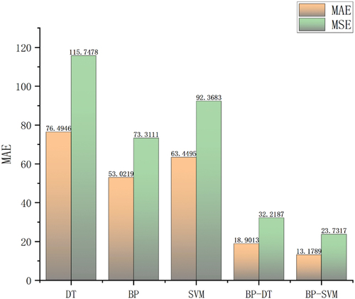
This chapter constructed and trained three prediction models: decision tree, support vector machine, and BP neural network, using 135 sets of data. The average absolute errors for the test sets of these models were 76.49, 53.02, and 63.44, respectively. Due to the influence of many uncertain factors, it is challenging to achieve predictions using a single method.

4.3. Combinatorial algorithm result

The algorithm was also executed on Matlab for the BP-DT-based cost prediction model, with the same data set ratio and evaluation metrics results shown in Table 5 and Figure 2.

Figure 2. Combined algorithm prediction results.

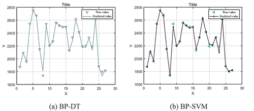
Table 5. Prediction results of the combination algorithm.

Algorithm	Training set MAE	Training set MSE	Test set MAE	Test set MSE
BP-DT	22.8516	39.9622	18.9013	32.2187
BP-SVM	9.2607	16.3149	13.1789	23.7317

Comparative analysis using the MAE and MSE evaluation metrics was conducted on the three single algorithm prediction models and two combined algorithm prediction models. The average absolute errors and mean squared errors of each model are shown in Figure 3. The prediction results indicate that, compared to the DT, BP, and SVM single algorithm prediction models, the BP-DT combined algorithm reduced the MAE by 72.16%, 64.35%, and 70.21%, and the MSE by 72.16%, 56.05%, and 65.12% respectively. The BP-SVM combined algorithm reduced the MAE by 82.77%, 75.14%, and 79.23%, and the MSE by 79.05%, 67.63%, and 74.31% respectively, compared to the single algorithms. Therefore, the combined machine learning algorithms significantly improve predictive performance compared to single machine learning algorithms. Among these two combined algorithms, BP-SVM outperformed BP-DT, with a 30.28% decrease in MAE and a 26.34% decrease in MSE.

Figure 3. Performance comparison of different prediction models.

4.4. Interpretative analysis results

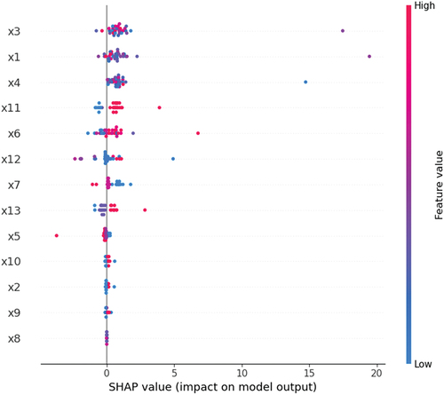
Figure 4 provides an in-depth insight into the factors influencing model predictions, displaying the contribution of different features to the model’s output. Features x1, x3, and x4 significantly impact the model’s output, evident from their wide and far-from-zero distribution of SHAP values. In contrast, the impact of features x8, x9, and x10 is relatively minor, with their SHAP values clustering close to zero. Additionally, the impact of features x6 and x12 fluctuates considerably across different data points, indicating inconsistent contributions to model predictions. For some features, such as x11 and x13, high values (red) are generally associated with an increase in model output, while low values (blue) correlate with a decrease. This analysis is crucial for understanding how the model processes different features, contributing to the transparency of the model’s decision-making process.

Figure 4. Sorting diagram of SHAP values.

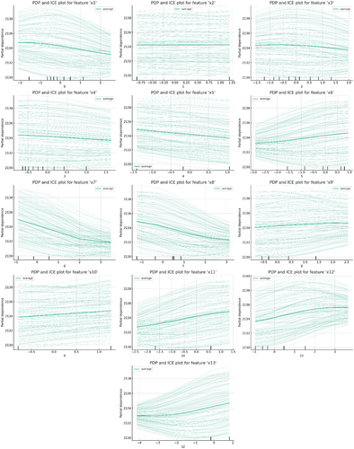
In the analysis of the provided Partial Dependence Plots (PDP) and Individual Conditional Expectation (ICE) plots, several key observations were made. Firstly, the PDP lines for many features are relatively flat, suggesting a limited average impact on model predictions, implying that the model’s predictions might be dominated by complex interactions among features rather than individual features. The ICE curves exhibit significant individual variation, indicating varied responses of the model to different samples, which may reflect the inherent heterogeneity of the data or non-linear relationships captured by the model. Certain features, such as x6, x9, and x12, exhibit a positive trend, implying that an increase in these feature values is associated with an increase in model predictions. In features like x1 and x13, the fan-shaped spread of ICE curves reveals non-linear characteristics, indicating that the model’s response to these features changes with different feature values (see as Figure 5). Additionally, some ICE curves significantly deviating from others may indicate potential outliers or influential points. Finally, features with PDP and ICE curves covering a wide horizontal range suggest significant variability of these features in the dataset. These findings underscore the importance of further statistical analysis, feature selection, and model tuning.

Figure 5. PDP and ICE charts for all features.

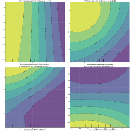
Figure 6 presents an analysis of the interactive effects of four sets of features. It was observed that when both Estimated project duration and Building form increase, the model’s predicted values seem to decrease, indicating a possible negative correlation between these two features. Conversely, lower values of these features correlate with higher model predictions. For the interaction between Estimated project duration and Exterior facade decoration, a relatively smooth transition is seen, where higher values of Exterior facade decoration appear to be associated with lower model predictions, especially when Estimated project duration is also high. This might suggest a mutually reinforcing negative effect when both features are at higher values. For the interaction between Estimated project duration and Interior decoration, high values of Estimated project duration and low values of Interior decoration seem to lead to an increase in model predictions, while low Estimated project duration and high Interior decoration result in decreased predictions. This indicates a possible offsetting effect between Estimated project duration and Interior decoration, where an increase in one feature and a decrease in another may lead to an increase in prediction outcomes. For the interaction between the Above-ground floor area and the Below-ground floors, the plot shows that higher model predictions occur when both features are at lower values, and predictions gradually decrease as the values of both features increase. This pattern may indicate an additive negative effect with the increase of both features.

Figure 6. Interactive influence diagram of features.

5. Conclusions

This study constructed cost prediction models for high-rise building engineering projects based on decision trees, BP neural networks, and support vector machine algorithms. Subsequently, an integrated cost prediction model for high-rise building engineering was established by fusing these three optimized prediction models using a weighted average method. The generalizability and predictive accuracy of the combined predictive algorithm were verified. The specific conclusions are as follows:

1. The combined algorithm effectively improves the predictive accuracy of the model, with the BP-SVM-based combined prediction algorithm being more suitable for the prediction study of high-rise building engineering costs.

2. Based on SHAP additivity analysis, it was concluded that “Estimated project duration” and “Ground floor area” are significant factors influencing the output. “Below-ground floors”, “Average above-ground floor height”, and “Average below-ground floor height” have the least impact.

3. Analysis of the model outputs using PDP and ICE plots revealed significant individual variation in the ICE curves, indicating diverse responses of the model to different samples. Through the analysis of feature interaction effects, it was found that “Estimated project duration” and “Building form” exhibit a certain negative correlation in their interaction; “Estimated project duration” and “Interior decoration” may have counteracting effects.

Disclosure statement

No potential conflict of interest was reported by the author(s).

Data availability statement

Data will be made available on request.

Additional information

Funding

This work is supported by the Ministry of Education of China and the National Innovative Training Program for College Students [202210153006].

Notes on contributors

Zenghui Liu

Liu Zenghui, a master’s student of intelligent building in Tianjin University, is engaged in the research of intelligent fire protection and intelligent engineering management.Jing Lin, Bachelor of Engineering, Master of Intelligent Building, Tianjin University, engaged in intelligent indoor environment research.

References

- Alshboul, O., A. Shehadeh, G. Almasabha, and A. S. Almuflih. 2022. “Extreme Gradient Boosting-Based Machine Learning Approach for Green Building Cost Prediction.” Sustainability 14 (11): 6651. https://doi.org/10.3390/su14116651.
- Arafa, M., and M. A. Alqedra. 2011. “Early Stage Cost Estimation of Buildings Construction Projects Using Artificial Neural Networks.” Journal of Artificial Intelligence 4 (1): 63–75. https://doi.org/10.3923/jai.2011.63.75.
- Bala, K., S. A. Bustani, and B. S. Waziri. 2014. “A Computer-Based Cost Prediction Model for Institutional Building Projects in Nigeria.” Journal of Engineering, Design & Technology 12 (4): 519–530. https://doi.org/10.1108/JEDT-06-2012-0026.
- Brandon, P. S. 1987. “Building Cost Modelling and Computers: Transactions of the Building Cost Research Conference on Building Cost Modelling and Computers.”
- Breiman, L. 2001. “Random Forests.” Machine Learning 45 (1): 5–32. https://doi.org/10.1023/A:1010933404324.
- Castro Miranda, S. L., E. Del Rey Castillo, V. Gonzalez, and J. Adafin. 2022. “Predictive Analytics for Early-Stage Construction Costs Estimation.” Buildings 12 (7): 1043. https://doi.org/10.3390/buildings12071043.
- Chandanshive, V., and A. Kambekar. 2019. “Estimation of Building Construction Cost Using Artificial Neural Networks.” Journal of Soft Computing in Civil Engineering: 3. https://doi.org/10.22115/scce.2019.173862.1098.
- Cheng, M.-Y., N.-D. Hoang, and Y.-W. Wu. 2013. “Hybrid Intelligence Approach Based on LS-SVM and Differential Evolution for Construction Cost Index Estimation: A Taiwan Case Study.” Automation in Construction 35:306–313. https://doi.org/10.1016/j.autcon.2013.05.018.
- Cheng, M.-Y., H.-C. Tsai, and E. Sudjono. 2010. “Conceptual Cost Estimates Using Evolutionary Fuzzy Hybrid Neural Network for Projects in Construction Industry.” Expert Systems with Applications 37 (6): 4224–4231. https://doi.org/10.1016/j.eswa.2009.11.080.
- Cherkassky, V., and Y. Ma. 2004. “Practical Selection of SVM Parameters and Noise Estimation for SVM Regression.” Neural Networks 17 (1): 113–126. https://doi.org/10.1016/S0893-6080(03)00169-2.
- Dong, S., X. Wu, X. Qi, C. Affolter, G. P. Terrasi, and G. Xian. 2023. “Prediction Model of Long-Term Tensile Strength of Glass Fiber Reinforced Polymer Bars Exposed to an Alkaline Solution Based on Bayesian Optimized Artificial Neural Network.” Construction and Building Materials 400:132885. https://doi.org/10.1016/j.conbuildmat.2023.132885.
- Du, T., J. Chen, F. Qu, C. Li, H. Zhao, B. Xie, M. Yuan, and W. Li. 2022. “Degradation Prediction of Recycled Aggregate Concrete Under Sulfate Wetting–Drying Cycles Using BP Neural Network.” Structures 46:1837–1850. https://doi.org/10.1016/j.istruc.2022.11.035.
- Ekanayake, I. U., D. P. P. Meddage, and U. Rathnayake. 2022. “A Novel Approach to Explain the Black-Box Nature of Machine Learning in Compressive Strength Predictions of Concrete Using Shapley Additive Explanations (SHAP).” Case Studies in Construction Materials 16:e01059. https://doi.org/10.1016/j.cscm.2022.e01059.
- Fan, C., N. Zhang, B. Jiang, and W. V. Liu. 2022. “Prediction of Truck Productivity at Mine Sites Using Tree-Based Ensemble Models Combined with Gaussian Mixture Modeling.” International Journal of Mining, Reclamation and Environment 37 (1): 66–86. https://doi.org/10.1080/17480930.2022.2142425.
- Fan, C., N. Zhang, B. Jiang, and W. V. Liu. 2023. “Weighted Ensembles of Artificial Neural Networks Based on Gaussian Mixture Modeling for Truck Productivity Prediction at Open-Pit Mines.” Mining, Metallurgy & Exploration 40 (2): 583–598. https://doi.org/10.1007/s42461-023-00747-9.
- Fan, M., and A. Sharma. 2021. “Design and Implementation of Construction Cost Prediction Model Based on SVM and LSSVM in Industries 4.0.” International Journal of Intelligent Computing and Cybernetics 14 (2): 145–157. https://doi.org/10.1108/IJICC-10-2020-0142.
- Glodon. 2022. https://www.gldzb.com/#/home.
- Hong, Y., H. Liao, and Y. Jiang. 2014. “Construction Engineering Cost Evaluation Model and Application Based on RS-IPSO-BP Neural Network.” Journal of Computers 9 (4): 1020–1025. https://doi.org/10.4304/jcp.9.4.1020-1025.
- Jas, K., and G. R. Dodagoudar. 2023. “Explainable Machine Learning Model for Liquefaction Potential Assessment of Soils Using XGBoost-SHAP, Soil Dynam.” Soil Dynamics and Earthquake Engineering 165:107662. https://doi.org/10.1016/j.soildyn.2022.107662.
- Joharestani, M. Z., C. Cao, X. Ni, B. Bashir, and S. Talebiesfandarani. 2019. “PM2.5 Prediction Based on Random Forest, XGBoost, and Deep Learning Using Multisource Remote Sensing Data.” Atmosphere 10 (7): 373.
- Kim, G. H., D. S. Seo, and K. I. Kang. 2005. “Hybrid Models of Neural Networks and Genetic Algorithms for Predicting Preliminary Cost Estimates.” Journal of Computing in Civil Engineering 19 (2): 208–211. https://doi.org/10.1061/(ASCE)0887-3801(2005)19:2(208).
- Kim, S., C. Y. Choi, M. Shahandashti, and K. R. Ryu. 2022. “Improving Accuracy in Predicting City-Level Construction Cost Indices by Combining Linear ARIMA and Nonlinear ANNs.” Journal of Management in Engineering 38 (2). https://doi.org/10.1061/(ASCE)ME.1943-5479.0001008.
- Li, S., T. Chen, L. Wang, and C. Ming. 2018. “Effective Tourist Volume Forecasting Supported by PCA and Improved BPNN Using Baidu Index.” Tourism Management 68:116–126. https://doi.org/10.1016/j.tourman.2018.03.006.
- Liu, G., H. Meng, G. Qu, L. Wang, L. Ren, and L. Fang. 2023. “Distributed Optical Fiber Sensor Temperature Dynamic Correction Method Based on Building Fire Temperature-Time Curve.” Journal of Building Engineering 68:106050. https://doi.org/10.1016/j.jobe.2023.106050.
- Liu, G., H. Meng, G. Qu, L. Wang, L. Ren, and H. Lu. 2023. “Real-Time Monitoring and Prediction Method of Commercial Building Fire Temperature Field Based on Distributed Optical Fiber Sensor Temperature Measurement System.” Journal of Building Engineering 70:106403. https://doi.org/10.1016/j.jobe.2023.106403.
- Liu, G., L. Ren, G. Qu, Y. Zhang, and X. Zang. 2022. “Fast Prediction Model of Three-Dimensional Temperature Field of the Commercial Complex for Entrance-Atrium Temperature Regulation.” Energy & Buildings 273:112380. https://doi.org/10.1016/j.enbuild.2022.112380.
- Lui, T. C. C., D. D. Gregory, M. Anderson, W. S. Lee, and S. A. Cowling. 2022. “Applying Machine Learning Methods to Predict Geology Using Soil Sample Geochemistry, Appl.” Applied Computing and Geosciences 16:100094. https://doi.org/10.1016/j.acags.2022.100094.
- Lundberg, S., and S. I. Lee. 2017. “A Unified Approach to Interpreting Model Predictions.” Proceedings of the 31st International Conference on Neural Information Processing Systems (NIPS’17). 4768–4777. Curran Associates Inc, Red Hook, NY.
- Qian, L., J. Zhao, and Y. Ma. 2022. “Option Pricing Based on GA-BP Neural Network.” Procedia Computer Science 199:1340–1354. https://doi.org/10.1016/j.procs.2022.01.170.
- Salling, K. B., and S. Leleur. 2015. “Accounting for the Inaccuracies in Demand Forecasts and Construction Cost Estimations in Transport Project Evaluation.” Transport Policy 38:8–18. https://doi.org/10.1016/j.tranpol.2014.11.006.
- Setvati, M. R., and S. J. Hicks. 2022. “Probabilistic Force Estimation and Event Localization (PFEEL) Algorithm.” Engineering Structures 252. https://doi.org/10.1016/j.engstruct.2021.113535.
- Sonmez, R. 2011. “Range Estimation of Construction Costs Using Neural Networks with Bootstrap Prediction Intervals.” Expert Systems with Applications 38 (8): 9913–9917. https://doi.org/10.1016/j.eswa.2011.02.042.
- Tehrany, M. S., B. Pradhan, and M. N. Jebur. 2013. “Spatial Prediction of Flood Susceptible Areas Using Rule Based Decision Tree (DT) and a Novel Ensemble Bivariate and Multivariate Statistical Models in GIS.” Journal of Hydrology 504:69–79. https://doi.org/10.1016/j.jhydrol.2013.09.034.
- Teng, S., N. Wu, H. Zhu, L. Teng, and W. Zhang. 2018. “SVM-DT-based Adaptive and Collaborative Intrusion Detection.” IEEE/CAA Journal of Automatica Sinica 5 (1): 108–118. https://doi.org/10.1109/JAS.2017.7510730.
- Thanikodi, S., M. Meena, Y. D. Dwivedi, T. Aravind, J. Giri, M. S. Samdani, L. Kansal, M. Shahazad, and M. Ilyas. 2024. “Optimizing the Selection of Natural Fiber Reinforcement and Polymer Matrix for Plastic Composite Using LS-SVM Technique.” Chemosphere 349:140971. https://doi.org/10.1016/j.chemosphere.2023.140971.
- Trost, S. M., and G. D. Oberlender. 2003. “Predicting Accuracy of Early Cost Estimates Using Factor Analysis and Multivariate Regression.” Journal of Construction Engineering and Management 129 (2): 198–204. https://doi.org/10.1061/(ASCE)0733-9364(2003)129:2(198).
- Vojinovic, Z., and V. Kecman. 2001. “Modeling Empirical Data to Support Project Cost Estimating: Neural Networks versus Traditional Methods.” Construction Innovation 1 (4): 227–243. https://doi.org/10.1108/14714170110814622.
- Wall, D. M. 1997. “Distributions and Correlations in Monte Carlo Simulation.” Construction Management & Economics 15 (3): 241–258. https://doi.org/10.1080/014461997372980.
- Wang, H., W. Zhou, and Y. Shao. 2024. “A New Fast ADMM for Kernelless SVM Classifier with Truncated Fraction Loss.” Knowledge-Based Systems 283:111214. https://doi.org/10.1016/j.knosys.2023.111214.
- Wang, K., J. Tian, C. Zheng, H. Yang, J. Ren, Y. L. Liu, Q. H. Han, and Y. B. Zhang. 2021. “Interpretable Prediction of 3-Year All-Cause Mortality in Patients with Heart Failure Caused by Coronary Heart Disease Based on Machine Learning and SHAP.” Computers in Biology and Medicine 137:104813. https://doi.org/10.1016/j.compbiomed.2021.104813.
- Xia, C., and G. Zhai. 2023. “Territorial Spatial Vulnerability Assessment Based on PSO-BP Neural Network: A Case Study in Shenzhen, China.” Ecological informatics 75:102088. https://doi.org/10.1016/j.ecoinf.2023.102088.
- Yuan, Y., G. Liu, R. Dang, S. S. Y. Lau, and G. Qu. 2021. “Architectural Design and Consumer Experience: An Investigation of Shopping Malls Throughout the Design Process.” Asia Pacific Journal of Marketing & Logistics 33 (9): 1934–1951. https://doi.org/10.1108/APJML-06-2020-0408.
- Zhang, Y.-F., W. Ren, W.-L. Wang, N. Li, Y.-X. Zhang, X.-M. Li, and W.-H. Li 2023. “Interpretable Hardness Prediction of High-Entropy Alloys Through Ensemble Learning.” Journal of Alloys and Compounds 无 945: 169329. https://doi.org/10.1016/j.jallcom.2023.169329.