Simulation of thermal effects due to different amounts of urban vegetation within the built-up area of Beijing, China

Abstract

Urban heat islands (UHI) are a common phenomenon in most cities, and one of the most effective ways to mitigate UHI negative effects is with urban vegetation. This paper uses the mono-window algorithm for retrieving land surface temperature (LST) based on remote-sensing data, and simulates thermal effects in five situations, using different amounts of urban vegetation within the built-up area of Beijing. Our analyses indicated that the computed Near Surface Air Temperature (NSAT) of the current situation (25 July 2005) was 295.86 K at 02:47 which is comparable to the real observed mean NSAT (296 K) at that time. When all urban vegetation was removed, the mean LST and NSAT increased by 1.95 K and 0.92 K compared to the current situation. In addition, the mean NDVI (normalized difference vegetation index) increased to 0.22–0.42, while the mean NSAT decreased to 294.98–293.08 K, which is close to a temperature comfortable to humans (295–293 K) in that area. Our work should provide information for the government of Beijing and the public on the importance of urban vegetation in counteracting effects of UHI during urban land use and management projects.

Keywords:

• urban heat island
• urban vegetation
• cooling effect
• land surface temperature
• near surface temperature
• Landsat 5 TM
• NDVI

Introduction

Urban heat islands (UHI) are a common phenomenon in cities worldwide (Akbari et al. 2001; Akbari 2005). UHI refers to the temperature of an urban area being higher than that of the surrounding rural area. The main cause of UHI is the alteration of energy balance (Oke 1982, 1988) within the urban area. This is done by replacing natural vegetation with construction to accommodate the growing population due to high rates of urbanization. This then results in abnormal temperature distribution, severe heat-related disease, high mortality rates (Kalkstein 1993; Semenza et al. 1996; Kalkstein and Greene 1997; Smoyer 1998), as well as high consumption of energy for air conditioning (Le Comte and Warren 1981; Santamouris et al. 2001). In order to increase the quality of life in urban areas, mitigation of the effects of UHI becomes a top priority for governments, researchers and the general public.

Among all cooling measures, urban vegetation is the most effective way to directly cool UHI, by providing shade and, indirectly, by plant evapotranspiration (Huang et al. 1987). Planting trees can effectively cool urban areas (Heisler 1977; Herrington 1977; Oke et al. 1989; Akbari et al. 1997; Streiling and Matzarakis 2003), and Spronken-Smith and Oke (1998) had verified the ‘park cool island’ (PCI) effect of vegetated urban parks. Moreover, urban vegetation can provide other ecosystem services, such as increased humidity, a balance between carbon dioxide and oxygen, air pollution reduction, aesthetic and recreation values, etc. (Bolund and Hunhammar 1999). Hence, urban vegetation is the primary cooling measure required in most cities.

As rapid urbanization takes place, more emphasis has been placed on the cooling effect of urban vegetation at a large scale, highlighting the importance of the involvement of government and the public in urban vegetation projects. Mesoscale meteorological models described by Taha et al. (1996, 1997) give us an understanding of the impacts of large-scale increases in albedo and vegetation on urban climate, helping to save energy used for air conditioning (Akbari et al. 2001). Most remote sensors carried by satellites can record thermal images and reflect spectral information of land cover temporally at a large scale. As the algorithms (Wan and Li 1997; Qin et al. 2001; Jimenez-Mun and Sobrino 2003) for retrieving land surface temperature (LST) from remote sensing thermal images matured, remote sensing has become a cost-effective technique to study temporal change in UHI and relationships with urban vegetation (Price 1979; Weng et al. 2004). Such studies provide a qualitative reference for the importance of the cooling effect of urban vegetation. Up to now, very few studies have reported quantitatively on how much vegetation is needed for urban areas to achieve comfortable temperatures for humans and how the removal of vegetation causes thermal change in the urban area. The answer to these questions can provide direct understanding of the cooling effect of vegetation on an urban scale.

This paper examines the negative relationship between the Normalized Difference Vegetation Index (NDVI) and the thermal infrared spectrum (Tian et al. 2006; Tran et al. 2006) of Landsat TM data. We employed the mono-window algorithm for retrieving land surface temperature based on remote-sensing data (Qin et al. 2001). Moreover, we carried out a simulation of thermal effects within an urban area containing different amounts of vegetation, using Beijing's built-up area as a case study. The paper attempts to quantitatively explore how temperatures change when all urban vegetation is removed and how much urban vegetation is required to cool the urban area, taking into consideration human comfort. Furthermore, the paper emphasizes the involvement of the Beijing government in urban vegetation planting and management, as well as participation of the public in urban green space planning and management.

Study area and data source

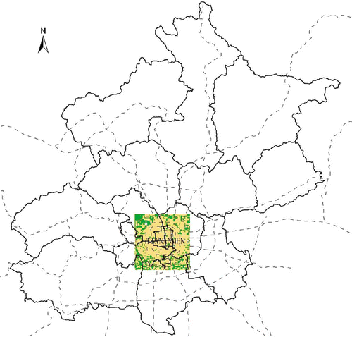
Beijing (39°56′N, 116°20′E) lies in northern China (Figure 1), and consists of eight districts and two counties. The total area is 16,808 km², and the total population is 14,000,000. The number of vehicles is over 3,000,000. The topography is mountainous in the northwestern part, accounting for one-third of the total land area, while the southeastern part consists of vast plains, accounting for the remaining two-thirds. The whole area from northwest to southeast belongs to the Haihe River watershed. The main rivers are Yongding River in the west and Chaobai River in the east, which has had no water for about half a century. The main wind direction is from southeast to northeast in summer, and the reverse during winter. Rainfall is about 600 mm/year. January is the coldest month with mean air temperature below 269 K, while July is the hottest month with mean air temperature over 297 K. Annually, the average air temperature is 284.6 K.

Figure 1. Beijing Municipal area and location of the study area.

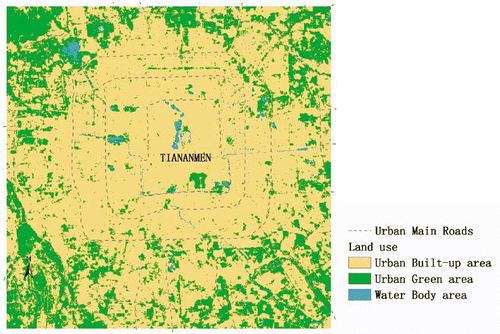
The Beijing urban built-up area is like a mono-centre pancake: centred on the Forbidden City and surrounded by the second, third, fourth, and fifth ring roads. Today, the built-up area exceeds 1000 km². To identify the thermal effect of the built-up area, our study focused on the city centre, with a total area of 900 km², within the plain area (Figure 1), where approximately seven million people work and live. Currently, the urban green area is about 230 km², including parks and other urban vegetation. The current land use is shown in Figure 2. With regard to urban development history, trend and the local climate, three Landsat 5 TM images from September of 1992 and July and November of 2005 were selected (Table 1).

Table 1. Characteristics of selected remote sensing image data

	Date (yyyy-mm-dd)	Numberof bands	Data type	Resolution(m)	Pass time
1	1992-09-07	7	Landsat 5 TM	30∗	02:47
2	2005-07-25	7	Landsat 5 TM	30∗	02:47
3	2005-11-14	7	Landsat 5 TM	30∗	02:47
Note: ∗the resolution of band 6 (infrared band) is 120 m.

Figure 2. Land use for the current situation.

Methods

Data pre-processing

All three Landsat 5 TM images (Table 1) were projected on to the UTM projection system and coordinated within the Beijing local coordinate system. A subset was then extracted by the AOI (Area of Interest) of the study area using ERDAS IMAGINE 8.5 software.

Calculation of NDVI and spectral radiance of the infrared band

Normalized difference vegetation index (NDVI)

NDVI mainly reflects the spectrum of vegetation, and is the indicator for growth states and richness of vegetation. We used it to calculate the amount of vegetation. NDVI maps were derived from all Landsat TM images listed in Table 1, using the computation shown below:

(1)

where R _NIR is the spectral reflectance of near-infrared, and R _Red is the red bands in the Landsat 5 TM data. This NDVI equation produces values ranging from −1 to 1, where positive values are rich vegetation; the higher the values, the richer the vegetation. In this study, NDVI was calculated using the NDVI module in ENVI 4.0 software.

Spectral radiance of the infrared band (TM6)

In the Landsat 5 TM image, band 6 is the thermal infrared band that can be used to calculate the bright temperature received by the sensor, revealing the temperature of the land surface. To calculate the spectral radiance of TM6 from the Digital Number (DN) value of the TM image, the following equation, developed by the National Aeronautics and Space administration (NASA) (Markham and Barker 1986), was used:

(2)

where L _(λ) is the spectral irradiance received by the sensor (mW cm⁻² sr⁻¹ um⁻¹), and Q _dn is the grey level for the analysed pixels of the TM image. In this study, while using the above equation, we applied the model maker tool of ERDAS IMAGINE 8.5 to calculate L _(λ) values of TM6.

Analysis of the regression relationship between NDVI and L_(λ) of TM6

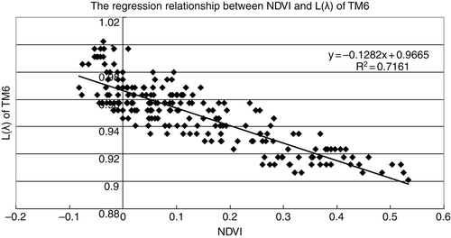
A number of studies have shown a negative correlation between NDVI and surface temperature (Tian et al. 2006; Tran et al. 2006) during summer. The L _(λ) of TM6 is the irradiance of surface temperature, therefore, there is also a negative correlation between NDVI and L _(λ) of TM6. In this study, we initially calculated NDVI and L _(λ) of TM6 of Landsat 5 TM data for July 25 2005. We then stacked the NDVI and L _(λ) of TM6 maps together using the ERDAS software tool. After this, we sampled 208 pairs of values of NDVI and L _(λ) of TM6 in the map by grid code. While sampling, we did not use any waterbody because there is no negative correlation between NDVI and L _(λ) of TM6 of waterbodies (Yuan and Bauer 2007). Finally, we were able to complete the regression analysis of the relationship of the 208 pairs of values using SPSS 13.0 software.

Simulation of thermal effects

We simulated thermal effects by calculating the LST and near surface air temperature.

Calculation of LST

We applied the Mono-window algorithm for retrieving land surface temperature from Landsat TM data, which was developed by Qin et al. (2001). The formulae are presented below:

(3)

(4)

(5)

where T _s is the LST, a = 67. 355351, b = 0.1458606; and ε is the ground emissivity, which can be calculated as (Qin et al. 2004):

• For a waterbody ε = 0.995

For natural vegetation surface, which is a combination of vegetation and bare soil, the formula is:

(6)

where ε_v, ε_s are the emissivities of vegetation and bare soil, ε_v = 0. 986 and ε_s = 0.97215; r _v, r _s are the temperature ratios of vegetation and bare land, which can be calculated using the following formula:

(7)

(8)

where p _v is the percentage of vegetation within a pixel, and the calculation is as follows (Carlson and Ripley 1997):

(9)

where NDVI_min = 0.05 refers to the entire bare surface, and NDVI_max = 0.70 refers to the entire vegetation surface, if NDVI > NDVI_max then p _v = 1, and if NDVI < NDVI_max then p _v = 0.

For the built-up area surface, which is a combination of vegetation and buildings, the formula is:

(10)

where ε_m are emissivities of buildings, ε_m = 0.986; and r _m are temperature ratios of buildings, the calculation of which is:

(11)

where τ is the is the atmospheric transmittance, which can be calculated as:

(12)

where w is water vapor content (g cm⁻²), w = 0.57 g cm⁻² according to historical records.

T _a is the effective mean atmospheric temperature, which can be calculated as:

(13)

where T ₀ is the mean surface air temperature (K) during a satellite pass according the historical record on 25 July 2005, T ₀ = 296 K.

T _sensor is the effective at-satellite brightness temperature (K), which can be calculated as:

(14)

where L _(λ) is spectral radiance received by the sensor (mW cm⁻² sr⁻¹ um⁻¹), which can be calculated from Equation (2)(2).

With the above formulae, we were able to calculate the LST for all five situations with different amounts of urban vegetation.

Calculation of near-surface air temperature (NSAT)

Concerning air temperature, which people feel directly, we calculated the LST. Thereafter, we calculated the near-surface air temperature (NSAT) at a height of 1.5 m from the linear regression relationship between LST and 1.5 m near-surface air temperature, as developed by Kawashima et al. (2000). The computations are as:

(15)

where T _a(1.5 m) is height at 1.5 m near-surface air temperature (K); T _s is LST (K).

After T _a(1.5 m) was calculated, we randomly sampled 10 values in the T _a(1.5 m) map, and made interpolations using the 10 values into the isolines of near-surface air temperature for every situation proposed.

Scenarios proposed and their parameters

Looking at urban development history and possible future policies in Beijing, not taking into account the current situation, we presumed four scenarios with different amounts of urban vegetation within the built-up area.

Scenario 1

We call this Bare City, because all the urban vegetation is removed within the built-up area of Beijing. This most severe situation would happen if there are no strict policies to manage construction, especially if there is no awareness of the importance of urban vegetation by the government and general public. The values of vegetation cover and NDVI are listed in Table 2.

Table 2. Description and the variables of the five situations

	Scenario 1: Bare City (BC)	Scenario 2: UnhealthyVegetation City (UVC)	Current situation: Current City (CC)	Scenario 3: Pre-Developed City (PDC)	Scenario 4: Green City (GC)
Amount of urban vegetation	Nearly none	Winter 2005	Summer 2005	Summer 1992	High amount
Normalized difference vegetation index (NDVI)	< 0.05	−0.45–0.67, mean = 0.02 calculated from TM map data November 14, 2005	−0.19–0.61, mean = 0.12 calculated from TM map data July 25, 2005	−0.26–0.63, mean = 0.22 calculated from TM map data September 07, 1992	>0.4
Spectral radiance of TM band 6 (L (λ))	From the linear regression between NDVI and L (λ) ( Equation (1)(1))		From band 6 of TM map data July 25, 2005	From linear regression between NDVI and L (λ) ( Equation (1)(1))
Land surface temperature (T s)	Mono-window algorithm for retrieving land surface temperature from Landsat TM data (Qin et al. 2001)
1.5 m air temperature (T a(1.5 m))	Linear regression between T s and T a(1.5 m) (Kawashima et al. 2000)

Scenario 2

We call this Unhealthy Vegetation City, wherein the area of urban vegetation is the same as that of the current situation (25 July 2005), but the health of such vegetation is very poor. If Beijing were to suffer any water shortage or extreme weather, most of the vegetation would die or be in very poor condition. We used the NDVI of Landsat 5 TM image during winter of 2005 (14 November 2005) to represent urban vegetation in this situation.

Scenario 3

We call this Pre-developed City. As we know, the Beijing urban built-up area has developed like a mono-centre pancake. Historically, it was much smaller than its current size, and was surrounded by a suburban area with rich vegetation. Inside the built-up area, vegetation cover was even higher than in the current situation. We used the NDVI of Landsat 5 TM image for summer 1992 (7 September 1992) to represent the urban vegetation of this situation, which also contained the first Green Belt rectified by the Beijing Government. This scenario would occur if government implements the first Green Belt and promotes the Tree Planting programme.

Scenario 4

We call this Green City, where there is rich urban vegetation within the built-up area. An extreme situation would occur if the Beijing Government promotes the Tree Planting programme and a green vegetation roof on top of most buildings within this area: vegetation cover could reach 40%, and the NDVI would be higher than 0.4.

Including the current situation, we have a total of five situations with different amounts of urban vegetation within the built-up area (Table 2).

Results and discussion

Regression relationship between NDVI and radiance of TM6

Figure 3 shows that there is a strong negative relationship (R ² = 0.7161) between the value of NDVI and the radiance of TM6 on 25 July 2005, which is in agreement with earlier studies (Jang et al. 2006; Tian et al. 2006). By using this analysis, we developed the linear regression model:

Figure 3 Regression relationship between NDVI and radiance of TM6.

(16)

where L _(λ) is the spectral radiance of TM6 (mW cm⁻² sr⁻¹ um⁻¹).

Reliability analysis of the model and thermal characterization of the current situation

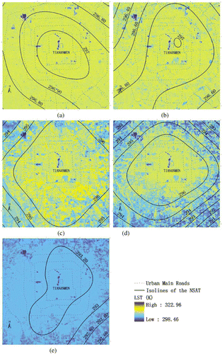
Using the methods shown above, we computed the LST and NSAT of the current situation based on Landsat 5 TM data for 25 July 2005 (Figure 6). The computed mean NSAT in the current situation was 295.86 K during the time of pass of the Landsat 5 satellite (02:47). This is comparable to the real observed mean NSAT (296 K) at that time, which verified the model. Through distribution of LST and NSAT in the summer of 2005, the UHI was very strong (about 3 K difference between the mean NSAT at the centre of the city and that in the outskirts area at night), and comparable to Song and Zhang (2003) values for 40 years of UHI study in Beijing. The maximum LST reached 322.96 K and the maximum NSAT reached 301.53 K, which both mainly occurred in the centre of the city (impervious surface) and in the industrial area in the southeast (dark roof with strong artificial heat emission). The low LST and NSAT were only found in the centre and around the urban parks with rich urban vegetation scattered within the built-up area. The lowest LST and NAST were 298.46 K and 290.51 K, found in a waterbody within an urban park.

Figure 6. Distribution of Land Surface Temperature (LST) and isolines of Near Surface Air Temperature (NSAT) within the Beijing built-up area in the five situations. (a) Bare City; (b) Unhealthy Vegetation City; (c) Current City; (d) Pre-Developed City; (e) Green City.

Thermal change in the built-up area in five situations

Maximum, mean and minimum LST and NSAT

Table 3 and Figure 4 show the maximum, mean and minimum LST in the five situations, and Table 4 and Figure 5 show the maximum, mean and minimum NSAT, also in the five situations. Generally, from Green City to Bare City (a change of urban vegetation in Beijing built-up from a high amount to nearly no vegetation), the mean LST increased from 304.19 K to 312.40 K, and NSAT increased from 293.08 K to 296.78 K; the maximum LST and NSAT had the same trend as mean LST and NSAT in all situations, except the current situation. After examining the location of the maximum LST, in the southeast industrial area with high amounts of impervious surface, dark roofs and strong artificial heat emissions, the findings resulted in extreme maximum LST and NSAT. The minimum LST and NSAT in all situations remained at the same level around the waterbody, which resulted in exclusion of the waterbody in our simulation model because there was no significant relationship between NDVI and radiance of TM6 around it (Yuan and Bauer 2007).

Table 3. Maximum, mean and minimum LST in the five situations

Situation	Min LST (K)	Mean LST (K)	Max LST (K)	SE (K)
Green city	298.46	304.19	304.82	0.7
Pre-developed city	298.45	308.41	315.14	3.72
Current city	298.46	310.35	322.96	3.07
Unhealthy city	298.45	311.97	317.31	1.94
Bare city	298.45	312.4	317.31	1.52

Table 4. Maximum, mean and minimum NSAT in the five situations

Situation	Min NSAT (K)	Mean NSAT (K)	Max NSAT (K)	SE (K)
Green city	290.51	293.08	293.37	0.31
Pre-developedcity	290.5	294.98	298.01	1.67
Current city	290.51	295.86	301.53	1.38
Unhealthycity	290.5	296.59	298.99	0.87
Bare city	290.51	296.78	298.99	0.69

Figure 4. Maximum, mean and minimum LST in the five situations.

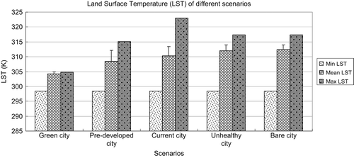
Figure 5. Maximum, mean and minimum NSAT in the five situations.

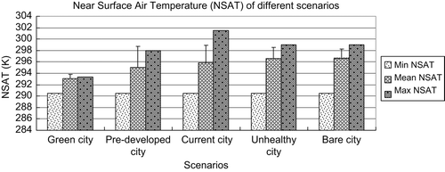
Specifically, from Current City to Unhealthy Vegetation City, then to the Bare City scenario, mean LST rose from 310.35 K to 312.4 K, while mean NSAT rose from 295.86 K to 296.78 K. Therefore, if all the urban vegetation was taken away or became unhealthy (mean NDVI decrease from 0.12 to 0.00), the mean LST and NSAT would increase by 1.95 K and 0.92 K at night. This is comparable to the historical increase in mean air temperature for 20 years in this area (Song and Zhang 2003). From Current City to Pre-developed City, then the Green City scenario, mean LST decreased from 310.35 K to 304.19 K, and mean NSAT decreased from 295.86 K to 293.08 K. If the government promotes urban vegetation planting and green roof programmes, the mean NDVI will increase from 0.12 to 0.22–0.42 and the mean NSAT will decrease from 295.86 K to 294.98–293.08 K, which is close to the human comfort temperature (295–293 K).

Distribution of LST and isolines of NSAT in the five situations

Figure 6 shows the distribution pattern of LST and isolines of NSAT in the five situations. It was not difficult to identify the UHI effect of LST and NSAT. Generally (Figure 6a–e), the UHI effect of LST and NSAT gradually decreased. The LST of the Bare City scenario (Figure 6a) remained almost the same inside and outside of the study area, except for the waterbody. The LST of the Unhealthy Vegetation City (Figure 6b) was almost the same as that in the Bare City scenario, with some Park Cooling Islands (PCI) provided by urban parks scattered throughout the area. With regard to the isolines of NSAT (Figure 6a and b), the area enclosed by the isoline 296.80 K in Figure 6a was larger than that in Figure 6b, which may have resulted from the PCI effect. The LST of the Current City (Figure 6c) scenario decreased from the inside to the outside of the study area, with extreme high LST scattered around the industrial area and the PCI effect around urban parks and waterbodies. The UHI of NSAT differed by about 3 K between the inside and the outside. The LST of the Pre-Developed City scenario (Figure 6d) also decreased from the inside to the outside of the study area. The difference in UHI of NSAT inside and outside was also about 3 K. Comparing Figure 6c and d, we found that as urban growth increases, more natural vegetation is replaced by construction containing impervious surfaces. This results in a stronger UHI of NSAT for the area enclosed by the isoline 296 K in Figure 6c, which is larger than that in Figure 6d. The LST and NSAT of the Green City scenario (Figure 6e) almost remained at the same level inside and outside of the study area, and there was almost no UHI of LST and NSAT inside and outside of the area.

Cooling effect of urban vegetation in the five situations

Figure 7 shows the regression relationship between mean NDVI and mean NSAT of the five situations, showing that there was a large negative relationship between them (R ² = 0.9973). The regression formula is:

(17)

where mean NSAT is the mean near surface air temperature of the built-up area in Beijing, and mean NDVI is the mean normalized difference vegetation index.

Figure 7. Co-relationship analysis between mean NDVI and mean NSAT of the five situations.

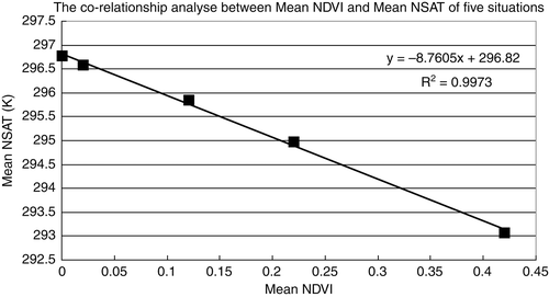
Using Equation (17)(17), we could forecast air temperature as urban vegetation changes within the built-up area, which provides a reference to the Beijing government and public for urban land use and management.

Conclusions

In accordance with the urban development history and potential development trend of Beijing, this study simulated the thermal effect of the built-up area of Beijing caused by different amounts of urban vegetation in order to investigate the cooling effect of vegetation. The results were obtained by combining the regression model between NDVI and L _(λ) of TM6, mono-window algorithm for retrieval of LST, and the regression model between LST and NSAT. Such results proved reliable, even in simulation of thermal effects under the same condition of sun irradiance and local climate. After removing all vegetation from the built-up area, the mean LST and NSAT increased by 1.95 K and 0.92 K compared to the current situation, which emphasizes the importance of urban vegetation for counteracting UHI. While increasing the mean NDVI from 0.12 to 0.22–0.42, the mean NSAT decreased from 295.86 K to 294.98–293.08 K, which is close to the human comfort temperature (295–293 K). These results address the question on how much urban vegetation should be planted within the built-up area of Beijing. Our study also established a visual relationship between temperature and urban vegetation, which could encourage public participation in urban land use and management. Further studies should consider the pattern and other ecosystem services of urban vegetation to confirm the need for vegetation within built-up areas in order to improve human well-being.

Acknowledgements

We thank the following foundations for support, the National Nature Science Foundation of China (70,433,001) and the Knowledge Innovation Project of The Chinese Academy of Sciences (KZCX2-YW-422 and KZCX2-YW-324). We would also like to thank the staff of the Research Centre of Eco-Environmental Sciences, CAS and the reviewers who helped improve this paper.

References

- Akbari , H . . Potentials of urban heat island mitigation . International Conference Passive and Low Energy Cooling for the Built Environment . Santorini, Greece. pp. 11 – 22 . May 2005
- Akbari , H , Kurn , DM , Bretz , SE and Hanford , JW . 1997 . Peak power and cooling energy savings of shade trees . Energy Build. , 25 : 139 – 148 .
- Akbari , H , Pomerantz , M and Taha , H . 2001 . Cool surfaces and shade trees to reduce energy use and improve air quality in urban areas . Solar Energy. , 70 : 295 – 310 .
- Bolund , P and Hunhammar , S . 1999 . Ecosystem services in urban areas . Ecol Econ. , 29 : 293 – 301 .
- Carlson , TN and Ripley , DA . 1997 . On the relation between NDVI, fractional vegetation cover, and leaf area index . Remote Sens Environ. , 62 : 241 – 252 .
- Heisler , GM . 1977 . Trees modify metropolitan climate and noise . J Arboric. , 3 : 201 – 207 .
- Herrington , LP . 1977 . The role of urban forests in reducing urban energy consumption . Proceedings of the Society of American Foresters Conference, Washington, D.C. , : 60 – 66 .
- Huang , YJ , Akbari , H , Taha , H and Rosenfeld , A . 1987 . The potential of vegetation in reducing summer cooling loads in residential buildings . Clim ApplMeteorol. , 26 : 1103 – 1116 .
- Jang , ZY , Chen , YH and Li , J . 2006 . Heat island effect of Beijng based on Landsat TM data . Geom Inf Sci Wuhan Univ. , 31 : 120 – 123 . In Chinese
- Jimenez-Mun , JC and Sobrino , JA . 2003 . A generalized single-channel method for retrieving land surface temperature from remote sensing data . J Geophys Res. , 108 : 4688 – 4695 .
- Kalkstein , LS . 1993 . Health and climate change – direct impacts in cities . Lancet. , 342 : 1397 – 1399 .
- Kalkstein , LS and Greene , JS . 1997 . An evaluation of climate/mortality relationships in large U.S. cities and the possible impacts of a climate change . Environ Health Perspect. , 105 ( 1 ) : 84 – 93 .
- Kawashima , S , Ishida , T , Minomura , M and Miwa , T . 2000 . Relations between surface temperature and air temperature on a local scale during winter nights . J Appl Meteorol. , 39 : 1570 – 1579 .
- Le Comte , DM and Warren , HE . 1981 . Modeling the impact of summer temperatures on national electricity consumption . J Appl Meteorol. , 20 : 1415 – 1419 .
- Markham , BL and Barker , JL . 1986 . “ Landsat-MSS and TM post calibration dynamic ranges, atmospheric reflectance and at-satellite temperature ” . In EOSAT Landsat Technical Notes. 1 , 3 – 8 . Lanham, , Maryland : Earth Observation Satellite Company .
- Oke , TR . 1982 . The energetic basis of the urban heat island . Q J R Meteorol Soc. , 108 : 1 – 24 .
- Oke , TR . 1988 . The urban energy balance . Prog Phys Geogr. , 12 : 471 – 508 .
- Oke , TR , Crowther , JM , McNaughton , KG , Monteith , JL and Gardiner , B . 1989 . The micrometeorology of the urban forest . Philos Trans R Soc Lond. , 324 : 335 – 349 .
- Price , JC . 1979 . Assessment of the urban heat island effect through the use of satellite data . Mon Weather Rev. , 107 : 1554 – 1557 .
- Qin , ZH , Karnieli , A and Berliner , P . 2001 . A mono-window algorithm for retrieving land surface temperature from Landsat TM data and its application to the Israel–Egypt border region . Int J Remote Sens. , 22 : 3719 – 3746 .
- Qin , ZH , Li , WJ , Xu , B and Zhang , WC . 2004 . Estimation method of land surface emissivity for retrieving land surface temperature from Landsat TM6 data . Adv Mar Sci. , 22 : 129 – 137 . In Chinese
- Santamouris , M , Papanikolaou , N , Livada , I , Koronakis , I , Georgakis , C , Argiriou , A and Assimakopoulos , DN . 2001 . On the impact of urban climate on the energy consumption of buildings . Solar Energy. , 70 ( 3 ) : 201 – 216 .
- Semenza , JC , Rubin , CH , Falter , KH , Selanikio , JD , Flanders , WD , Howe , HL and Wilhelm , JL . 1996 . Heat-related deaths during the July 1995 heat wave in Chicago . N Engl J Med. , 335 ( 2 ) : 80 – 90 .
- Smoyer , KE . 1998 . A comparative analysis of heatwaves and associated mortality in St. Louis, Missouri – 1980 and 1995 . Int J Biometeorol. , 42 : 44 – 50 .
- Song , YL and Zhang , SY . 2003 . Sudy on heat island effects in Beijing during last 40 years . Chin J Eco-Agric. , 11 : 126 – 129 . In Chinese
- Spronken-Smith , RA and Oke , TR . 1998 . The thermal regime of urban parks in two cities with different summer climates . Int J Remote Sens. , 19 : 2085 – 2104 .
- Streiling , S and Matzarakis , A . 2003 . Influence of single and small clusters of trees on the bioclimate of a city: a case study . J Arboric. , 29 : 309 – 316 .
- Taha , H , Douglas , S and Haney , J . 1997 . Mesoscale meteorological and air quality impacts of increased urban albedo and vegetation . Energy Build (Special Issue on Urban Heat Islands and Cool Communities). , 25 : 169 – 177 .
- Taha , H , Konopacki , S and Gabersek , S . 1996 . Modeling the meteorological and energy effects of urban heat islands and their mitigation: a 10-region study , Berkeley, CA : Lawrence Berkeley Laboratory Report LBL- 38667 .
- Tian , ZK , Huang , MF , Liu , LY , Zhu , QJ and Zhao , CJ . 2006 . Study on Beijing urban heat effect with Landsat ETM data and mono-window algorithm . Remote Sens. Inf. , 1 : 21 – 24 . In Chinese
- Tran , H , Uchihama , D , Ochi , S and Yasuoka , Y . 2006 . Assessment with satellite data of the urban heat island effects in Asian megacities . Int J Appl Earth Observ Geoinf. , 8 : 34 – 48 .
- Wan , Z and Li , ZL . 1997 . A physics-based algorithm for retrieving land-surface emissivity and temperature from EOS/MODIS data . IEEE Trans. Geosci. Remote Sens. , 35 : 980 – 996 .
- Weng , Q , Lu , D and Schubring , J . 2004 . Estimation of land surface temperature–vegetation abundance relationship for urban heat island studies . Remote Sens Environ. , 89 : 467 – 483 .
- Yuan , F and Bauer , ME . 2007 . Comparison of impervious surface area and normalized difference vegetation index as indicators of surface urban heat island effects in Landsat imagery . Remote Sens Environ. , 106 : 375 – 386 .