Availability and distribution of environmental education field trip programs for adolescent students in the U.S.: a national study of spatial accessibility

Abstract

What is the availability and distribution of single-day environmental education field trip programs for adolescent students across the U.S.? We assessed the spatial accessibility to EE field trip programs for U.S. schools that serve grades 5-8 (ages 10-14) by (1) compiling a comprehensive national database of 2,930 EE providers that offer field trip programs, (2) identifying 89, 311 middle schools’ locations, student populations, and relevant demographic information, and (3) calculating drive times between schools and EE provider locations using a high-performance computing cluster. We then used the integrated Floating Catchment Area method to calculate each school’s relative spatial access to EE field trip providers. Results suggest that spatial access was highly spatially clustered, particularly around several geographic regions (coastal California metropolitan areas, the southern Rockies, northern Kentucky, North Carolina, the western shore of Lake Michigan, and the high-density, contiguous metropolitan areas of the Northeast). Spatial access was also strongly related to partisan lean and urbanity, with more rural, White, and Republican-leaning areas generally having significantly less spatial access to EE field trips.

Keywords:

• Spatial Accessibility
• constraints
• Environmental education
• barriers to participation
• Education

1. Introduction

The field of environmental education (EE) aims to cultivate awareness, appreciation, and understanding of the natural environment as well as the attitudes, skills and motivations needed to address challenges associated with climate change, pollution, and environmental degradation (Crutzen 2006; IPCC 2021; UNESCO 1977). Effective EE programs have been shown to influence each of these outcomes in addition to social-emotional learning, academic achievement, and general satisfaction and enjoyment (Ardoin et al. 2018; Powell et al. 2019; Stern, Powell, and Hill 2014). While EE programs can range from brief interactions to multi-day excursions for a wide variety of audiences, much of the field focuses on educating youth, especially student groups (Ardoin et al. 2018). In the United States, these programs commonly are comprised of school field trips for students, lasting a day or less in duration. This particular form of EE has the potential to serve a broader cross-section of the public than more costly programs such as multi-day and overnight programs and are offered in wide array of contexts (e.g. Stern, Powell, and Frensley 2022).

Despite the broad benefits and commonly low costs of EE field trip programs, attending a field trip program requires schools to overcome a range of potential barriers, including transportation challenges and other costs associated with attending; perceptions about the alignment of curricula and standards of learning; cultural factors related to obtaining parental permission; teachers’ attitudes toward the experience; and bureaucratic and administrative challenges (Stern, Wright, and Powell 2012; Xiao et al. 2017; Anderson, Kisiel, & Storksdieck, 2006). While each of these barriers to EE accessibility has been identified through prior research, spatial accessibility (supply, distribution, and travel times) may also limit participation. We know of no large-scale investigation of the spatial accessibility (supply, distance, and travel time) of single-day EE field trip providers for schools across the U.S. Thus, the purpose of this paper is to investigate spatial access to day-long EE field trips for adolescent youth (grades 5-8) across the U.S. by addressing the following research questions:

1. Is spatial access to EE field trips for students in grades 5-8 (ages 10-14) equitably distributed across the U.S.?

2. If spatial access to EE field trips for students in grades 5-8 (ages 10-14) is inequitably distributed:

   1. Which areas have significantly greater or lesser spatial access?

   2. Is spatial access related to sociodemographic (rurality, socioeconomic status, race) and cultural context (political)?

We focus our study on spatial accessibility of EE field trips for grades 5-8 because of their prevalence in the U.S and these ages, (10-14), represent a critical period of cognitive and moral development in which children generally develop higher-level thinking, stronger connections to nature, and important twenty-first century skills (Ardoin et al. 2018; Kahn and Kellert 2002; Kohlberg 1979; Piaget 1964).

2. Literature review: spatial accessibility

Spatial accessibility represents both the availability (supply) of a resource as well as its accessibility (distance and travel time) (Guagliardo 2004; Penchansky and Thomas 1981). Concepts of accessibility, as well as increasingly sophisticated methods of its measurement, have developed primarily in the medical field. Though the bulk of investigations and advancements have emerged from healthcare studies, researchers have adapted and expanded accessibility modeling in a diversity of other contexts, including green space and natural protected areas (Chang and Liao 2011; Li et al. 2019; Tan and Samsudin 2017; Wang, Brown, and Liu 2015; Wen et al. 2013; Wu et al. 2020; Xiao et al. 2018), ecosystem services (Ala-Hulkko 2020; Ala-Hulkko et al. 2016), food deserts (Bao et al. 2020; Dai and Wang 2011), banks (Langford, Higgs, and Jones 2021), schools and childcare (Chen, Zhou, and Yeh 2020; Fransen et al. 2015; Talen 2001), public transit (Jomehpour Chahar Aman and Smith-Colin 2020; Lee, Sohn, and Heo 2018), casinos (Papineau et al. 2020), and fire stations (Kc, Corcoran, and Chhetri 2020).

Spatial accessibility measurement began simply. At first, the ratio of resource availability to the size of the population within defined geographic regions, such as city or state boundaries, was used as the standard metric (e.g. supply/demand, population density, or per capita calculations). In the accessibility literature, this is known as the “container approach” or, in the healthcare context, the population-to-provider ratio. This sort of metric is familiar to most and remains useful and appropriate in many contexts. However, it fails to account for the permeable nature of the area’s boundaries. People’s use of resources like hospitals or, in our study, EE providers is not limited by political boundaries (i.e. they are permeable). A middle school class in Kansas City, Missouri is not barred from, or likely to avoid, attending an EE field trip at a nature center across town in Kansas City, Kansas just because it is technically located in another city, county, and state. This is a well-known problem in geographic research referred to as the modifiable areal unit problem, or, MAUP (Fotheringham and Wong 1991).

The “gravity model” was developed to address the MAUP. This model assumes that human movement and spatial activity mirror Newton’s law of gravitation, meaning that the “pull” of an available resource on an individual is driven by its nearness and “attractiveness,” or, size (e.g. the closer and larger the hospital, the more likely it is to be used). The gravity model has been generalized and applied to diverse human behavior, from retail decisions to migration and transportation, and was popularized as a metric of spatial accessibility by Hansen (1959), Weibull (1976), and Joseph and Bantock (1982). Although gravity models of spatial accessibility are still used by some researchers (Chang and Liao 2011; Zhang, Lu, and Holt 2011), and they are an improvement over container-based ratios, the basic gravity model is limited by the difficulty of determining the correct gravity decay function (β; how does the pull of the resource diminish over distance) and by the lack of adjustment for a population’s demand (Guagliardo 2004).

Luo and Wang (2003) were the first to propose a special case of the gravity model that they called the Two-Step Floating Catchment Area method (2SFCA). Their basic formulation and numerous extensions and variations have become the state-of-the-art method in spatial accessibility studies. Known collectively as FCA (floating catchment area) methods, they essentially function by applying the simple supply/demand ((S_y/P_x) ratio to a “catchment area” around each supply location (y) that is defined by a maximum reasonable travel distance (C_glob) and calculated using the sum of demand at all population locations (x) that fall within the catchment area. The equation then sums the newly calculated supply/demand ratios of those supply locations that fall within each population location’s own catchment area, thus producing a spatial accessibility index value for every population location (AI_x). The method can be depicted in the following formula and visually as in Figure 1: $${AI}_x=\mathrm{ }{\sum }_{y\in (d_{xy}\le C_{\mathit{glob}})}\frac{S_y}{{\sum }_{x\in (d_{xy}\le C_{\mathit{glob}})}{P}_x}$$

Figure 1. Visualization of the basic 2SFCA method applied to the EE field trip context, adapted from Ye et al. (2018).

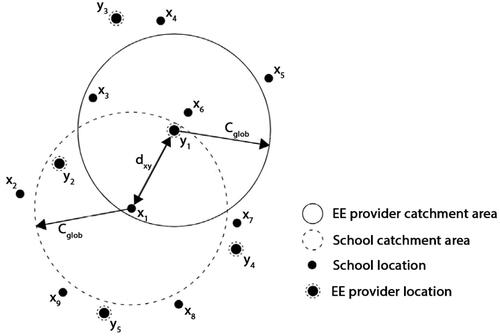
FCA methods have clear advantages over earlier models of spatial accessibility. Most importantly, they can be interpreted in the same way as the simple supply/demand ratio. They also account for both supply and demand within a meaningful areal unit that is fitted to each individual supply and demand location (i.e. maximum reasonable travel distance). In the basic 2SFCA formulation, however, several deficiencies still remain, and many researchers consider it too simplistic (McGrail and Humphreys 2009; Saxon and Snow 2020). These critiques are that: (1) the model’s catchment areas, while meaningful, remain fixed even though maximum reasonable travel distance from a population location (or, willingness to travel) would likely vary based on the presence or absence of nearby supply; (2) no distance decay function is included, even though we would expect individuals to prefer nearer supply over that which is farther away; and (3) competition between supply locations for the finite demand of a population location is ignored, even though demand at a supply location would obviously be higher if it were the only supply in the area rather than if multiple supply locations were present (Bauer and Groneberg 2016; Saxon et al. 2022; Wan, Zou, and Sternberg 2012).

A suite of variations and extensions of the 2SFCA model have been proposed to address these limitations. Most frequently, investigators have made improvements by incorporating a variety of distance decay functions into the model (Bryant and Delamater 2019; Dai and Wang 2011; Hu et al. 2020; Luo and Qi 2009; Wu et al. 2020), Several authors have also incorporated variable catchment areas (Luo and Whippo 2012; McGrail and Humphreys 2014) and functions to account for competition (Luo 2014; Wan, Zou, and Sternberg 2012).

For our analysis we have chosen to use an FCA method developed by Bauer and Groneberg (2016) that integrates and improves on the advancements made by other versions of the FCA, which they call the integrated Floating Catchment Area method (iFCA). It does so by: (1) applying a logistic distance decay function that is shaped individually for each population location using the standard deviation and median of population-to-provider distances within a global maximum catchment area; (2) calculating an effective catchment area size for each population location defined by each density decay function’s asymptotic approach to zero; and (3) incorporating the Huff model (Huff 1964) to account for competition between supply locations. We consider this model to be the most advanced currently in use.

3. Methods

The intent of our investigation is to assess the spatial accessibility to single-day EE field trip programs for schools that serve grades 5-8 in the United States. To do so, we: (1) compiled a national database of EE providers that offer programs of this type, (2) identified middle schools’ locations, student populations, and relevant demographic information from the National Center for Education Statistics, and (3) used a high-performance computing cluster to calculate drive times between schools and EE provider locations at scale. Next, we used the integrated Floating Catchment Area method to calculate each school’s relative spatial access to EE field trip providers. Then we identified meaningful spatial and demographic trends in this data using a set of common statistical analyses.

3.1. EE provider locations

At the time of the study, no complete national database of EE providers existed. While some state-level lists and databases had been compiled by state agencies or North American Association for Environmental Education (NAAEE) affiliate organizations, many other states had no such information available. Moreover, even where they did exist, many contained out-of-date or partial information. Consequently, we compiled our own database. We attempted to identify all EE providers that deliver single-day field trip programming for students in grades 5-8. We followed the same search and compilation procedure for EE providers in all 50 states (and Washington, D.C.) to avoid systematically over- or under-representing any one of them. This also ensured that, should any deficiencies exist in our search procedure, they were equally present across the study area.

Our dataset was compiled between February 2020 and May 2022 by extensively checking countless potential providers’ web sites for evidence that they offered field trip programs that meet our inclusion criteria (that is, the potential provider offered single-day field trip programs for student groups in grades 5-8). For each state we identified as many potential providers as possible for evaluation using the following steps:

1. We identified 37 state level EE provider databases and lists. We reviewed all provider’s webpages to ensure compliance with our inclusion criteria.

2. Several state NAAEE affiliates did not have a database but contacted their listservs and requested provider information on our behalf.

3. We reviewed the websites for all units of relevant U.S. federal agencies (National Park Service, Forest Service, U.S. Fish and Wildlife Service, National Oceanic and Atmospheric Administration, Bureau of Land Management, Army Corp of Engineers) for compliance with our inclusion criteria.

4. We reviewed the websites for all units of relevant state agencies (including conservation districts and departments of state parks and preserves, agriculture, forestry, fishing, wildlife, natural resources, conservation, and environmental protection) for compliance with our inclusion criteria.

5. Comprehensive lists of many of the most common EE provider types existed on Wikipedia for each state. All such lists were exhaustively checked for compliance with our inclusion criteria. They were:

6. Nature centers (https://en.wikipedia.org/wiki/List_of_nature_centers_in_the_United_States)

7. Botanical gardens and arboretums (https://en.wikipedia.org/wiki/List_of_botanical_gardens_and_arboretums_in_the_United_States)

8. Zoos (https://en.wikipedia.org/wiki/List_of_zoos_in_the_United_States)

9. Aquaria (https://en.wikipedia.org/wiki/List_of_aquaria_in_the_United_States)

10. Science centers (https://en.wikipedia.org/wiki/List_of_science_centers_in_the_United_States)

11. Natural history museums (https://en.wikipedia.org/wiki/List_of_natural_history_museums_in_the_United_States)

12. Farm museums (https://en.wikipedia.org/wiki/Category:Farm_museums_in_the_United_States)

13. Environmental research institutes (https://en.wikipedia.org/wiki/List_of_environmental_research_institutes#United_States)

14. Smithsonian Institute affiliates (https://en.wikipedia.org/wiki/Category:Smithsonian_Institution_affiliates)

15. Wildlife rehabilitation and conservation centers (https://en.wikipedia.org/wiki/Category:Wildlife_rehabilitation_and_conservation_centers)

16. Fish hatcheries (https://en.wikipedia.org/wiki/Category:Fish_hatcheries_in_the_United_States)

17. If any of the previous steps led to the discovery of additional lists of EE providers (e.g., city/local area provider lists), these providers, too, were systematically checked against our inclusion criteria.

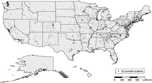
This procedure produced our final national dataset of EE providers (n = 2,930) (Figure 2). While we acknowledge that this dataset is inevitably incomplete, we believe it represents the most comprehensive snapshot of providers of single-day EE field trip programs ever developed in the United States.

Figure 2. Locations of EE providers in the U.S. that offer single-day field trip programming for students in grades 5-8 (n = 2,930).

3.2. School locations, populations, and sociodemographic data

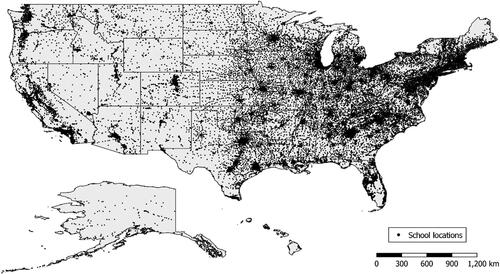
We identified middle schools’ locations, student populations, and relevant demographic information using databases made available by the National Center for Education Statistics (i.e.; the “Public Elementary/Secondary School Universe Survey,” “Private School Universe Survey,” and “Education Demographic and Geographic Estimates – Locale Classification”). All schools, both public and private, with any students in 5^th-8^th grade were included in our dataset (Figure 3). We also collected data on each school’s urbanity, total 5^th-8^th grade student population, percent of students receiving reduced or free lunches, and number of students representing each standard Census Bureau racial category. All data represented the 2019-2020 school year. This was the most recent school year with complete data for both public and private schools. We also calculated a metric of overall racial diversity using Shannon’s Index and student body racial data. Shannon’s diversity index has been used to quantify diversity across many contexts, most commonly in ecological studies, but also as a useful metric of racial and ethnic diversity in education research (Akay et al. 2017; McLaughlin, McLaughlin, and McLaughlin 2015; Morris et al. 2014; Shannon 1948). Additionally, we used FiveThirtyEight’s 2022 state-level “partisan lean” dataset (https://data.fivethirtyeight.com/) to explore the relationship between politics and access to EE field trips. This dataset represents partisan lean as the average difference between each state’s voting record and the voting record of the entire U.S., using for its calculation the results of the 2016 and 2020 presidential elections, as well as the statewide popular vote in the 2014, 2016, 2018, and 2020 state legislative elections.

Figure 3. Locations of schools in the U.S. with students enrolled in grades 5-8 (n = 83,911).

3.3. Global catchment area calculation

The global catchment size (C_glob)—defined in this study as the maximum drive time schools are willing to travel one way for a single-day field trip—is an important metric in the accurate estimation of a given resource’s spatial accessibility. Despite its importance, empirical data on the average maximum distance a study population would be willing to travel to access a particular resource is generally scarce. As a result, many are forced to use educated guesses, rules of thumb, or local knowledge (e.g. 30 min is often considered a reasonable threshold in the literature for people’s willingness to travel to a primary care physician; Guagliardo 2004; Luo 2014; McGrail and Humphreys 2014). Fortunately, however, our research team collected a robust dataset of schools in the U.S. that attended EE field trips (n = 138) as part of another study conducted in 2018 that focused on identifying the programmatic characteristics associated with more positive participant outcomes (see: Powell, Stern, and Frensley 2023; Dale et al. 2020; O’Hare et al. 2020; Stern, Powell, and Frensley 2022). Travel times between each school and the EE field trip provider that they visited were calculated using the routing engine described below (see Travel time calculations). In this nationwide sample, 95% of drive times for school-EE provider pairs (n = 133) were equal to or less than two hours, thus guiding our choice to set C_glob = 120 min.

3.4. Travel time calculations

In order to estimate spatial accessibility using FCA methods, the most critical—and computationally intensive—data needed is a matrix of origin-to-destination travel times. Nearly all school groups transport students to and from field trips on buses, so for this study we calculated a matrix of the time it takes to drive from all schools to all EE providers using the 5.26 release of the Open Source Routing Machine (OSRM), an open-source, high-performance C++ routing engine capable of rapidly calculating very large sets of origin-to-destination travel times (Luxen and Vetter 2011). We started by loading a Docker container of OSRM 5.26 onto Clemson University’s Palmetto High-Performance Computing Cluster using Singularity and the latest OpenStreetMap data extract for the complete U.S. road network. This procedure created a queryable “instance” of OpenStreetMap on the Palmetto Cluster, allowing us to feed the geographic coordinates of the schools and EE providers into the routing engine and calculate an origin-to-destination travel time matrix (Table 1). We then amended the resulting matrix to include only those school-EE provider pairs whose travel time was two hours or less, producing a dataset of the travel times from every school to every EE field trip provider that falls within the global maximum willingness-to-travel threshold (C_glob) of each school.

Table 1. Travel time matrix calculation steps.

	# of calculations	O-D pairs removed
83,910 schools * 2,930 EE providers (travel time from every school to every provider)	245,856,300	242,341,271
Travel time < = 2 h (global max. driving distance)	3,515,029	–

OpenStreetMap is a robust representation of the U.S. road network, so very little data cleaning was needed. Only in the rural communities of Alaska that are wholly inaccessible by road was a correction to calculated travel times necessary. In these cases, OSRM calculated the travel time between each EE provider and the point on the road network nearest to each of these road-inaccessible schools, which could be hundreds of kilometers away, rendering this value inaccurate and useless. For these schools, we corrected their distance to all EE providers, changing their matrix values to N/A, which most accurately indicated in the model that there were no EE providers available for these schools.

3.5. The iFCA model

Our iFCA model can be stated as follows, $${AI}_x=\mathrm{ }{\sum }_{y\in (d_{xy}\le C_x)}\frac{S_y\mathrm{*}{f}_{\mathit{adj}}\left(d_{xy}\right)\mathrm{*}{f}_{\mathit{con}}\left(d_{xy}\right)}{{\sum }_{x\in \left(d_{xy}\le C_x\right)}{P}_x\mathrm{*}{f}_{\mathit{adj}}\left(d_{xy}\right)\mathrm{*}{\mathit{Prob}}_{\mathit{demand}}}$$ where AI_x is an index of potential spatial access for school x, S_y is EE provider capacity at location y (S_y = 1 in all cases), P_x is the 5-8^th grade student population size at school x, f_adj(d_xy) is the adjusted and f_con(d_xy) the constant distance decay function applied to the distance d_xy between school x and EE provider location y. The distance decay functions take the following forms, $$f_{\mathit{adj}}\left(d_{xy}\right)=\mathrm{ }\frac{1+e^{-\left(\frac{\left(\mathit{Median}\right)\mathrm{*}\pi }{SD\mathrm{*}\sqrt{3}}\right)}}{1+e^{\frac{\left(d_{xy}-\mathit{Median}\right)\mathrm{*}\pi }{SD\mathrm{*}\sqrt{3}}}}$$ $$f_{\mathit{con}}\left(d_{x\mathrm{y}}\right)=\mathrm{ }\frac{1+e^{-\left(\frac{\left(\frac{C_{\mathit{glob}}}{2}\right)\mathrm{*}\pi }{{SD}_{\mathit{glob}}\mathrm{*}\sqrt{3}}\right)}}{1+e^{\frac{\left({d_{xy}-C}_{\mathit{glob}}/2\right)\mathrm{*}\pi }{{SD}_{\mathit{glob}}\mathrm{*}\sqrt{3}}}}$$ where Median is the median distance and SD the standard deviation of d_xy within the global catchment area (C_glob) around school x, and SD_glob is the global standard deviation where f_con(C_glob) = 0.01, which can be stated as $${SD}_{\mathit{glob}}=\mathrm{ }\frac{\pi \mathrm{*}\ln \hspace{0.17em}\left(e\right)\mathrm{*}{C}_{\mathit{glob}}}{2\mathrm{*}\sqrt{3}\mathrm{*}\ln \left(100\right)}$$

Finally, the probability of demand function, meant to account for competition and adapted from the Huff model (Huff 1964), can be stated as $${\mathit{Prob}}_{\mathit{demand}}=\mathrm{ }\frac{S_y\mathrm{*}{f}_{\mathit{adj}}\left(d_{xy}\right)}{{\sum }_{z\in \left(d_{xz}\le C_x\right)}{S}_z\mathrm{*}{f}_{\mathit{adj}}\left(d_{xz}\right)}$$ where the probability of demand from school x on EE provider y depends upon the presence of other EE providers z within the effective catchment area of school x (C_x)_.

3.6. Statistical analyses and data management

To statistically identify the spatial areas of high and low access to EE field trips, we used the Global Moran’s I test for spatial autocorrelation across the entire dataset and the Getis-Ord Gi* test for identifying statistically significant localized clusters of high and low values (i.e.; “hot” and “cold” spots). Much like ANOVA tests, the Global Moran’s I test is a “global” measure that describes the dataset as a whole—able to discern whether statistically significant clustering of access scores is present in the dataset, but unable to identify the specific clusters. Where post hoc tests would be used to solve this problem in ANOVA analyses, the Getis-Ord Gi* test is used here to identify the location and extent of these statistically significant clusters of high and low access. For Getis-Ord Gi* analyses, we used the “zone of indifference” conceptualization of spatial relationships (which combines features of inverse distance and fixed distance bands) and applied False Discovery Rate corrections to account for multiple testing and spatial dependence.

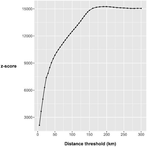
The Global Moran’s I statistic can be calculated at different spatial scales by using different distance thresholds. Additionally, z-scores from these tests can be compared to determine at which distance clustering is most intense, with higher scores indicating greater clustering. Here, we performed the calculation iteratively and incrementally across a wide range of distances to determine whether clustering of access to EE field trips is primarily local, regional, national, or cross-scalar and to identify appropriate distance thresholds for use in the Getis-Ord Gi* calculation. First, we calculated Global Moran’s I starting at 5 kilometers and increasing in 5 kilometer increments up to 150 kilometers, and then again starting at 150 kilometers and increasing in 10 kilometer increments up to 300 kilometers. Finally, spearman correlations, t-tests, ANOVAs, and linear regression were used to probe the relationships between sociodemographic factors and schools’ relative access. All data management and spatial and statistical analyses were conducted using ArcGIS, QGIS, R, SPSS, and Excel software.

4. Results

4.1. Schools’ spatial access to EE field trips

For schools with students in grades 5-8 across the United States (n = 83,911), spatial access to EE field trip providers was not evenly distributed (Figure 4a). Clusters of high access scores were immediately apparent in the Northeast, upper South and Southeast, Midwest, southern Rockies, and coastal California. Large expanses of low access were apparent across many rural regions of the country. The results of incremental spatial autocorrelation analysis (Global Moran’s I) confirm that this apparent spatial clustering of high and low access is both meaningful and cross-scalar, with Moran’s I being statistically significant at all measured distances (Figure 5). That is, high and low access scores are significantly concentrated in some regions of the country at the national scale, concentrated in some metropolitan areas at the regional scale, and concentrated in certain towns, counties, and neighborhoods at the local scale. To investigate this clustering at different spatial scales, we present Getis-Ord Gi* results that roughly depict “national” (Figure 4b), “regional” (Figure 4c), and “local” (Figure 4d) trends, wherein each school’s access score (AI_x) was compared to the access score of every other school within 200 kilometers, 75 kilometers, and 25 kilometers, respectively.

Figure 4. Maps depicting: (a) 5^th-8^th grade students’ relative spatial access to EE field trips at schools across the U.S.; (b-d) the Getis-Ord Gi* hot/cold spot statistic for schools’ access scores using neighborhood distance thresholds of: (b) 200 kilometers (national scale), (c) 75 kilometers (regional scale), and (d) 25 kilometers (local scale); and (e) schools (red dots) that have no access to EE field trips within a two hour drive.

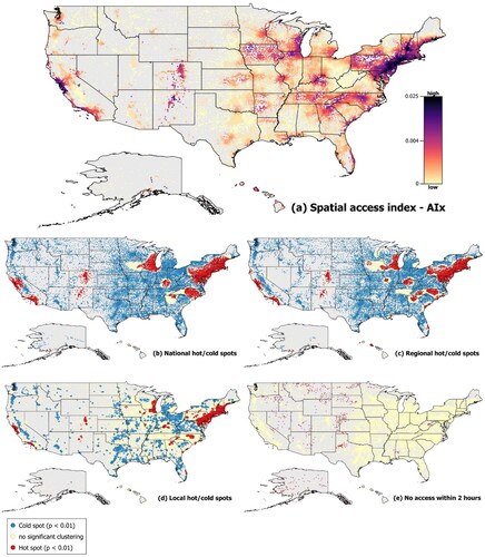
Figure 5. Z-scores for the Global Moran’s I statistic computed at various distances (n = 45), p < 0.001 in all cases. Higher z-scores indicate more intense clustering of high and low values.

At the national scale (Figure 4b), the Getis-Ord Gi* test reveals that the pattern of clustering depicts primarily high access concentrated in a handful of regions contrasted with low access concentrated everywhere else. At this scale of comparison, there are very few schools that do not form part of a high or low access cluster. The high-access “hearths” of EE field trips at this scale were (1) the northeastern urban agglomeration that stretches from Washington, D.C. to Boston, (2) western Lake Michigan (Chicago to Green Bay), (3) North Carolina & north Georgia, (4) Cincinnati-Louisville-Lexington, (5) the southern Rockies (Denver to Albuquerque), (6) the San Francisco Bay area, and (7) coastal southern California (Los Angeles to San Diego).

At the regional scale level (Figure 4c) the overall pattern of clustering does not change dramatically. Rather, many of the country’s schools remain in roughly the same expansive, low-access cluster as at the national scale. The national “hearths” of high EE field trip access roughly maintain shape but decompose somewhat to reveal high clustering in their constituent metropolitan areas (e.g.; the North Carolina-north Georgia cluster splits into distinct clusters centered around Atlanta, Asheville, Raleigh-Durham, and Wilmington), and several smaller regions of high access that lie outside of these “hearths” emerge (i.e.; Charleston, SC-Savannah, GA; St. Louis, MO; West Palm Beach, FL; Humboldt County, CA; Oahu, HI).

At the local scale (Figure 4d), the Getis-Ord Gi* test revealed that the large, contiguous cluster of low access splits and clarifies into numerous smaller cold spots. The test also revealed that the “hearths” of high access continue to maintain their rough shape although they now center on their metropolitan cores (e.g.; the southern Rockies hearth becomes distinct clusters of high access centered around Denver, Colorado Springs, Santa Fe, and Albuquerque). Furthermore, analyses at the local scale shows many schools, primarily in rural areas, no longer are a part of statistically significant high access clusters. Consequently, at this scale, clusters of particularly low access schools are distinguishable. In the western half of the contiguous U.S., these significant cold spots represent the majority of population centers that are not within a national hearth of high access. While in the eastern half, several regional clusters of low access are now distinguishable that could not be identified at the coarser scales of comparison (e.g.; the rough cluster stretching from the central Appalachians through the Rust Belt; north-central Florida; eastern Texas).

Finally, there are schools in our dataset that effectively have no access to EE field trip providers (within a two-hour drive of school grounds). These schools are located primarily in very rural, low-density regions of the U.S. (Figure 4e). In the West and Alaska, the majority of rural schools fall into this category, while in the East there are only four, very small clusters of schools with no access (i.e.; far northern Minnesota, southwestern Alabama, eastern West Virginia, and northern Maine).

4.2. Schools’ spatial access and student population characteristics

Spatial access to EE field trips, as represented by AI_x and the number of EE field trip providers within a two-hour drive, varies significantly between public and private schools and across schools’ relative urbanity (Table 2). Private schools have moderately higher access to EE providers (d = 0.26) and moderately more EE providers within a two-hour drive C_glob (d = 0.23), about six on average. Schools situated in “suburban” and “city” locales have about twice as much access to EE providers (η² = 0.10) and twice as many providers nearby (η² = 0.15) as schools in “rural” or “town” areas with a large effect-size.

Table 2. Descriptive statistics for schools’ key spatial access metrics and student body demographic characteristics for all schools combined, as well as grouped by their public/private status and urbanity. The results of statistical analyses comparing schools’ access to EE field trips (AI_x and total number of accessible EE providers) across their public/private status (t-test) and urbanity (ANOVA) are also provided.

	All schools (n = 83,911)	School type:		School urbanity:
		Public schools (n = 68,155)	Private schools (n = 15,756)	Rural (n = 22,474)	Town (n = 9,106)	Suburban (n = 27,240)	City (n = 25,063)
AIx		t (23257) = 19.75, p < 0.001, d = 0.26		F (3, 83879) = 3163, p < 0.001, η^2 = 0.10
mean (SD)	0.0025 (0.0028)	0.0025 (0.0027)	0.0029 (0.0028)	0.0014 (0.0022)	0.0014 (0.0017)	0.0034 (0.0029)	0.0031 (0.0029)
median (IQR)	0.0015 (0.0029)	0.0014 (0.0029)	0.0020 (0.0032)	0.0008 (0.0017)	0.0008 (0.0016)	0.0027 (0.0033)	0.0021 (0.0032)
range	0 − 0.1819	0 − 0.1819	0 − 0.025	0 − 0.1819	0 − 0.013	0 − 0.012	0 − 0.0123
# of EE providers		t (23054) = 17.16, p < 0.001, d = 0.23		F (3, 83879) = 5058, p < 0.001, η^2 = 0.15
mean (SD)	41.9 (41.4)	40.7 (41.1)	47.1 (42.5)	21.9 (23.6)	20.2 (19.1)	57.8 (44)	50.5 (46)
median (IQR)	27 (44)	26 (42)	31 (51)	16 (20)	16 (20)	44 (55)	32 (58)
range	0 - 197	0 – 197	0 - 195	0 - 185	0 - 169	0 - 196	0 - 197
Median time to EE providers
mean (SD)	73.1 (21.4)	73 (21.8)	73.6 (19.4)	81.4 (23.4)	82.6 (21.7)	68.9 (16.8)	66.8 (20)
median (IQR)	74.6 (28.6)	74.6 (29.1)	74.6 (26.6)	86.3 (23.9)	86.9 (23.5)	68.9 (23.7)	66.4 (27)
range	0 − 119.9	0 − 119.9	0 − 119.3	0 − 119.9	0 − 119.4	0 − 115.7	0 − 117.4
# of 5^th-8^th grade students
mean (SD)	194.6 (262.3)	224.7 (279.9)	64.6 (82.5)	143.3 (207.4)	194.9 (231.6)	233.3 (302.3)	198.6 (262.6)
median (IQR)	95 (150)	108 (186)	38 (72)	74 (116)	98 (208)	107 (173)	98 (154)
range	1 - 2531	1 – 2517	1 - 2531	1 - 2517	1 - 2001	1 - 2531	1 - 2449
% FRLP
mean (SD)	--	52.1 (29.9)	--	50 (26.3)	55.9 (25.4)	44.9 (30.1)	60.7 (32.1)
median (IQR)	--	52.7 (48.4)	--	49.7 (34.5)	56.1 (32.8)	42.4 (51.8)	69.3 (53.2)
range	--	0 – 100	--	0 - 100	0 - 100	0 - 100	0 - 100
Racial diversity
mean (SD)	0.68 (0.35)	0.7 (0.35)	0.63 (0.34)	0.49 (0.31)	0.58 (0.31)	0.78 (0.32)	0.79 (0.34)
median (IQR)	0.71 (0.57)	0.73 (0.57)	0.62 (0.55)	0.44 (0.51)	0.58 (0.5)	0.82 (0.48)	0.84 (0.49)
range	0 − 1.67	0 − 1.64	0 − 1.67	0 − 1.67	0 − 1.44	0 − 1.61	0 − 1.65
% White
mean (SD)	51.5 (32.9)	49.3 (32.9)	62.9 (30.1)	72.5 (27.2)	64.7 (28.6)	48.4 (30.2)	32.1 (28.7)
median (IQR)	56.5 (62.8)	52.4 (64)	72.2 (43.1)	83.5 (32.9)	74 (42.9)	52.4 (55.4)	25 (51.1)
range	0 - 100	0 – 100	0 − 99.9	0 - 100	0 - 100	0 - 100	0 - 100
% Black
mean (SD)	14.4 (22.9)	15 (23.3)	11.6 (20.3)	6.8 (15.5)	8.4 (17.7)	14.1 (20.3)	23.6 (28.5)
median (IQR)	4.1 (15.4)	4.1 (16.8)	3.9 (10)	1.1 (4.6)	1.5 (5.5)	5.7 (14.8)	10.4 (31.1)
range	0 - 100	0 – 100	0 − 99.8	0 - 100	0 - 100	0 - 100	0 - 100
% Hispanic
mean (SD)	23.1 (26.5)	25.1 (27.2)	13.2 (19.7)	12.3 (18.8)	18.7 (24)	25.3 (26)	31.8 (29.7)
median (IQR)	11.5 (29.1)	13.4 (32.5)	5.5 (13)	5 (11.4)	8.2 (21)	14.8 (30.5)	20.2 (45)
range	0 - 100	0 – 100	0 − 99.8	0 - 100	0 - 100	0 - 100	0 - 100
% Asian/Pacific Islander
mean (SD)	4.4 (9.4)	4.1 (8.9)	5.7 (11.3)	1.2 (4.1)	1.3 (3.1)	6.3 (10.5)	6.2 (11.6)
median (IQR)	1.2 (4)	1 (3.5)	2.1 (5.9)	0.2 (1)	0.6 (1.3)	2.6 (6.1)	2 (5.9)
range	0 - 100	0 – 100	0 − 99.1	0 - 100	0 − 63.5	0 − 99.1	0 - 100
% Native American
mean (SD)	1.5 (8)	1.6 (8.4)	0.8 (5)	3.4 (13.8)	2.2 (8.8)	0.4 (1.8)	0.7 (2.7)
median (IQR)	0.1 (0.5)	0.2 (0.6)	0 (0)	0 (0.6)	0.2 (0.7)	0.1 (0.4)	0.2 (0.5)
range	0 - 100	0 – 100	0 − 98.6	0 - 100	0 - 100	0 − 86.5	0 - 100
% Hawaiian
mean (SD)	0.4 (2.6)	0.4 (2.4)	0.6 (3.4)	0.3 (2.6)	0.5 (3.6)	0.4 (2.4)	0.5 (2.3)
median (IQR)	0 (0.2)	0 (0.2)	0 (0)	0 (0)	0 (0.1)	0 (0.3)	0 (0.3)
range	0 - 100	0 – 100	0 − 85.2	0 - 100	0 - 100	0 − 85.2	0 − 81.7

Spearman rank correlation analyses further reveal that all tested student body characteristics (race, % FRLP, and # of students) are significantly correlated with schools’ relative access to EE providers, though all of these relationships are fairly weak (Table 3). Larger student populations, greater racial diversity, and greater proportions of Black, Hispanic, Asian/Pacific Islander, and Hawaiian students are associated with greater access to EE field trips, while greater proportions of students that are White, Native American, and eligible for free and reduced lunch are associated with less access to EE field trips.

Table 3. Spearman correlation matrix for key spatial access metrics and student body demographic characteristics.

	AIx	# of EE providers	Median time to EE providers	# of 5^th-8^th students	% FRLP	Racial diversity	% White	% Black	% Hispanic	% Asian/ Pacific Islander	% Native American	% Hawaiian
AIx	1	.87***	−0.14***	.07***	−0.12***	.19***	−0.17***	.21***	.10***	.33***	−0.14***	.05***
# of EE providers		1	−0.09***	.11***	−0.08***	.25***	−0.27***	.29***	.20***	.37***	−0.16***	.07***
Median time to EE providers			1	−0.06***	.00	−0.17***	.29***	−0.10***	−0.21***	−0.22***	−0.07***	−0.15***
# of 5^th-8^th students				1	−0.04***	.15***	−0.12***	.11***	.18***	.21***	.16***	.20*
% FRLP					1	−0.01	−0.52***	.25***	.33***	−0.25***	.08***	.01
Racial diversity						1	−0.41***	.51***	.48***	.59***	.27***	.35***
% White							1	−0.53***	−0.65***	−0.17***	−0.11***	−0.17***
% Black								1	.12***	.15***	−0.01	.10***
% Hispanic									1	.20***	.15***	.21***
% Asian/Pacific Islander										1	.09***	.30***
% Native American											1	.21***
% Hawaiian												1

* p-values < 0.05, ** p-values < 0.01, *** p-values < 0.001.

Partisan lean is significantly and strongly associated with schools’ median spatial access to EE field trips at the state level, r(49) = .73, p < .001. This association is visually apparent in Figure 6, in which states’ access to EE is displayed in descending order according to their relative partisan lean, from most Democratic-leaning to most Republican-leaning states. With the exception of states like Washington, Oregon, Iowa, Kentucky, and Tennessee, students in Democratic-leaning states have significantly greater access to EE field trips, on average, than do students in Republican-leaning states.

Figure 6. Density plots of AI_x, along with median AI_x, for each state. Density plots are ordered by states’ partisan lean in recent elections (displayed numerically to the right of the graph), with states that have leaned most heavily towards Democratic candidates at the top and those that have leaned most heavily towards Republican candidates at the bottom.

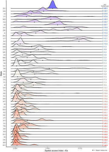
The distribution of spatial access to EE field trips also differs from state to state, with some states like North Dakota, Utah, Rhode Island, and Washington, D.C. having relatively little variation in AI_x, and others like Maryland, California, New York, and Pennsylvania exhibiting relatively high variation (Figure 6). Additionally, while some states have a unimodal distribution, many others have bimodal or trimodal distributions. These multimodal distributions indicate states in which distinct clusters of higher and lower access are present. For example, Kentucky’s bimodal distribution reflects the cluster of higher access around the Louisville-Lexington area in contrast with the lower access elsewhere in the southern and eastern portions of the state (Figure 4). Likewise, California’s trimodal distribution reflects the high access clusters in its coastal metropolitan areas (Los Angeles, San Diego, and the Bay Area), low access in the Central Valley, and moderate access everywhere else.

Finally, we regressed schools’ spatial access to EE field trips on school and student body characteristics, thus producing a well-fitted, statistically significant model that explains 35% of variation in AI_x across our dataset (Table 4). When considered together, race and school type have significant but relatively weak relationships with access to EE field trips, while urbanity and partisan lean have significant and relatively strong relationships with access.

Table 4. Linear regression of AI_x on key school characteristics; F (9, 81509) = 4874, p < 0.001, r² = 0.35. ‘% White’ was dropped from the model due to extremely high multicollinearity with the other independent variables and ‘% FRLP’ was not included because it only exists for public schools. Negative signs indicate less access; positive signs indicate greater access.

	B	S.E.	B	t	p-value	VIF
Intercept	0.002111	0.0000256		82.521	<0.001
% Black	0.000007	0.0000004	0.059	18.493	<0.001	1.19
% Hispanic	−0.000007	0.0000003	−0.074	−22.240	<0.001	1.28
% Asian/Pacific Islander	0.000023	0.0000010	0.079	23.411	<0.001	1.32
% Native American	−0.000011	0.0000010	−0.031	−10.460	<0.001	1.04
% Hawaiian	−0.000052	0.0000031	−0.051	−17.005	<0.001	1.03
Racial diversity	0.000162	0.0000262	0.021	6.185	<0.001	1.33
Urbanity (binary)*	0.001017	0.0000198	0.184	51.443	<0.001	1.47
Public (binary)^	−0.000263	0.0000221	−0.037	−11.887	<0.001	1.09
State-level partisan lean^‡	0.000060	0.0000005	0.422	130.904	<0.001	1.19

* = suburban/urban (1) and rural/town (0); ^ = public (1) and private (0);

‡ = continuous scale in which Democratic lean is positive and Republican lean negative divergence from zero.

5. Discussion

The purposes of this study was to explore whether spatial access to day-long EE field trips for students in grades 5-8 is equitably distributed across the U.S., to identify clusters of high and low access, and to examine whether spatial access is related to sociodemographic context. We used state-of-the-art spatial analysis techniques in conjunction with high-performance computing systems to produce an extensive, fine-grained portrait of the relative spatial access to single-day EE field trips across the U.S.

Our series of analyses at multiple scales (national, regional, and local levels) provide a series of increasingly fine-grained analyses to provide an overall picture of spatial access to single-day EE field trip programs for adolescent youth. Overall, we found that spatial access were highly spatially clustered, particularly around several geographic regions (coastal California metropolitan areas, the southern Rockies, northern Kentucky, North Carolina, the western shore of Lake Michigan, and the high-density, contiguous metropolitan areas of the Northeast). Spatial access was also strongly related to partisan lean and urbanity, with more rural, White, and Republican-leaning areas generally having significantly less spatial access to EE field trips.

These results lend deeper insight into the claim that BIPOC youth have less access to EE programming (Children & Nature Network 2016). More specifically, our findings suggest that issues related to diversity, equity, inclusion, and access for BIPOC youth appear to be primarily aspatial in nature and stem from other issues such as historic systemic racism, multi-generational poverty, and inequitable educational opportunities (Devine 2019; Hong and Anderson 2006; Lawrence Hall of Science 2019; Rose and Paisley 2012; Le and Holmes 2012; Romero et al. 2022).

At the state level, relative outliers among Republican-leaning states, Iowa and Tennessee, may offer a template for increasing access to EE field trip opportunities. In Iowa, the majority of County Conservation Boards offer standards-aligned EE field trip opportunities for local schools. Because there is one of these offices located in each county, universal access to at least one EE field trip provider within a two-hour drive of school is virtually ensured. In Tennessee, equitably/universally distributed access has been achieved through the state park system, which offers EE field trips to school groups. Possible providers in other states that could enhance spatial access to EE programming include State Park systems, Natural Resource Conservation Service (NRCS), libraries, or school district-employed educators in partnership with local outdoor public spaces, to name a few viable options. Direct state funding or financial incentives could be offered to train existing institutional employees, promote these new field trip opportunities, and otherwise support the program. While these interventions alone would not resolve nationwide disparities in access, even one to two nearby options could go a long way toward reducing the prevalence of extreme “cold spots” and complete lack of access, as teachers in the U.S. typically only take students on an average of about 1-2 field trips per school year (Kenna 2019; Kenna and Russell 2015; Muse, Chiarelott, and Davidman 1982; Whitesell 2016).

While our analysis is the most robust assessment of nationwide spatial access to single-day EE field trip programs for adolescent youth to date, several limitations and suggestions for future studies should be considered. First, our study did not account for EE providers’ maximum student capacity. Rather, the availability of EE field trips was represented by presence/absence at any given location. A basic estimate of each provider’s relative student capacity (e.g. “large,” “medium,” and “small” EE providers)—or even better, an estimate of the maximum number of students that an EE provider could accommodate in a day or week—would produce a much more finely-tuned estimate of schools’ relative spatial access to EE field trips. Second, some EE field trip providers were undoubtedly missed by our search procedures. The U.S. is a large country and some providers have much less public exposure or internet presence than others. Third, our study had a narrow focus on day-long EE field trips. We did not account for online EE programs, residential and multi-day field trip programs, and programs for other ages. As such, the results cannot be generalized beyond single-day field trip programs for middle school students (ages 10-14). For example, Oregon provides funding to support universal access to residential multi-day environmental education programming for 5-6^th graders (Sobel 2017; Powell et al. 2019). In our results, Oregon appeared to have less access to programs even though students across the state have access to these multi-day programs. Future studies that incorporate a broader array of offerings, as well as younger and older audiences, would greatly improve understanding of overall spatial access to EE. Finally, all of our analyses are correlational measures that do not offer any indication of what forces shape the relative allocation of EE field trip sites.

6. Conclusion

Despite the limitations discussed above, the study identified clear trends, elucidating issues related to the availability and spatial distribution of day-long EE field trip programs. Overall, the results indicate that urban and suburban students have greater spatial accessibility to these programs. Thus, explanations of variable attendance in these areas are likely attributable to aspatial barriers such as cost, transportation, limited marketing, cultural barriers, and perceptions regarding meeting curriculum standards (e.g. Stern, Wright, and Powell 2012). Our results also indicate that many rural students and schools have little to no access to EE field trip programs. EE advocates should consider focusing efforts in these “spatial accessibility deserts” to address spatial inequities and identify viable strategies for increasing the availability of EE for rural youth.

Additional information

Funding

The funding for the study was provided by the National Science Foundation’s Advancing Informal STEM Education program (DRL 1906610).

References

- Akay, A., A. Constant, C. Giulietti, and M. Guzi. 2017. “Ethnic Diversity and Well-Being.” Journal of Population Economics 30 (1): 265–306. https://doi.org/10.1007/s00148-016-0618-8
- Ala-Hulkko, T. 2020. “Integrating Accessibility Analysis in Ecosystem Service and Disservice Mapping [University of Oulu].” Nordia Geographical Publications 49: 73. https://nordia.journal.fi/article/view/97279.
- Ala-Hulkko, T., O. Kotavaara, J. Alahuhta, P. Helle, and J. Hjort. 2016. “Introducing Accessibility Analysis in Mapping Cultural Ecosystem Services.” Ecological Indicators 66: 416–427. https://doi.org/10.1016/j.ecolind.2016.02.013
- Anderson, D., J. Kisiel, and M. Storksdieck. 2006. “Understanding Teachers’ Perspectives on Field Trips: Discovering Common Ground in Three Countries.” Curator: The Museum Journal 49 (3): 365–386.
- Ardoin, N. M., A. W. Bowers, N. W. Roth, and N. Holthuis. 2018. “Environmental Education and K-12 Student Outcomes: A Review and Analysis of Research.” The Journal of Environmental Education 49 (1): 1–17. https://doi.org/10.1080/00958964.2017.1366155
- Bao, K. Y., D. Tong, D. A. Plane, and S. Buechler. 2020. “Urban Food Accessibility and Diversity: Exploring the Role of Small Non-Chain Grocers.” Applied Geography 125 (June): 102275. https://doi.org/10.1016/j.apgeog.2020.102275
- Bauer, J., and D. A. Groneberg. 2016. “Measuring Spatial Accessibility of Health Care Providers – Introduction of a Variable Distance Decay Function within the Floating Catchment Area (FCA) Method.” PloS One 11 (7): e0159148. https://doi.org/10.1371/journal.pone.0159148
- Bryant, J., and P. L. Delamater. 2019. “Examination of Spatial Accessibility at Micro- and Macro-Levels Using the Enhanced Two-Step Floating Catchment Area (E2SFCA) Method.” Annals of GIS 25 (3): 219–229. https://doi.org/10.1080/19475683.2019.1641553
- Chang, H. S., and C. H. Liao. 2011. “Exploring an Integrated Method for Measuring the Relative Spatial Equity in Public Facilities in the Context of Urban Parks.” Cities 28 (5): 361–371. https://doi.org/10.1016/j.cities.2011.04.002
- Chen, Z., X. Zhou, and A. G. Yeh. 2020. “Spatial Accessibility to Kindergartens Using a Spectrum Combinational Approach : Case Study of Shanghai Using Cellphone Data.” Urban Analytics and City Science 48 (6): 1380–1397. https://doi.org/10.1177/2399808320954221
- Children & Nature Network. 2016. From Research to Practice: Connecting Children to Nature Executive Summary of Findings from a Survey of Environmental Educators. https://naaee.org/eepro/resources/connecting-children-nature-executive
- Crutzen, P. J. 2006. “The “Anthropocene.” In Earth System Science in the Anthropocene, 13–18. Berlin, Heidelberg: Springer.
- Dai, D., and F. Wang. 2011. “Geographic Disparities in Accessibility to Food Stores in Southwest Mississippi.” Environment and Planning B: Planning and Design 38 (4): 659–677. https://doi.org/10.1068/b36149
- Dale, R. G., R. B. Powell, M. J. Stern, and B. A. Garst. 2020. “Influence of the Natural Setting on Environmental Education Outcomes.” Environmental Education Research 26 (5): 613–631. https://doi.org/10.1080/13504622.2020.1738346
- Devine, J. A. 2019. “The Rise of the American Conservation Movement: Power, Privilege, and Environmental Protection.” Gender, Place & Culture 26 (3): 447–449. https://doi.org/10.1080/0966369X.2017.1409943
- Fotheringham, A. S., and D. W. S. Wong. 1991. “The Modifiable Areal Unit Problem in Multivariate Statistical Analysis.” Environment and Planning A: Economy and Space 23 (7): 1025–1044. https://doi.org/10.1068/a231025
- Fransen, K., T. Neutens, P. De Maeyer, and G. Deruyter. 2015. “A Commuter-Based Two-Step Floating Catchment Area Method for Measuring Spatial Accessibility of Daycare Centers.” Health & Place 32: 65–73. https://doi.org/10.1016/j.healthplace.2015.01.002
- Guagliardo, M. F. 2004. “Spatial Accessibility of Primary Care: Concepts, Methods and Challenges.” International Journal of Health Geographics 3 (1): 3. https://doi.org/10.1186/1476-072X-3-3
- Hansen, W. G. 1959. “How Accessibility Shapes Land Use.” Journal of the American Institute of Planners 25 (2): 73–76. https://doi.org/10.1080/01944365908978307
- Hong, A., and D. H. Anderson. 2006. “Barriers to Participation for Latino People at Dodge Nature Center.” The Journal of Environmental Education 37 (4): 33–44. https://doi.org/10.3200/JOEE.37.4.33-44
- Hu, S., W. Song, C. Li, and J. Lu. 2020. “A Multi-Mode Gaussian-Based Two-Step Floating Catchment Area Method for Measuring Accessibility of Urban Parks.” Cities 105 (May 2019): 102815. https://doi.org/10.1016/j.cities.2020.102815
- Huff, D. L. 1964. “Defining and Estimating a Trading Area.” Journal of Marketing 28 (3): 34–38. https://doi.org/10.2307/1249154
- IPCC. 2021. Climate Change 2021: The Physical Science Basis. Contribution of Working Group I to the Sixth Assessment Report of the Intergovernmental Panel on Climate Change [Masson-Delmotte, V., P. Zhai, A. Pirani, S. L. Connors, C. Péan, S. Berger, N. Caud, and Y. Chen]. Cambridge University Press, 3949. https://www.ipcc.ch/report/ar6/wg1/downloads/report/IPCC_AR6_WGI_Full_Report.pdf
- Jomehpour Chahar Aman, J., and J. Smith-Colin. 2020. “Transit Deserts: Equity Analysis of Public Transit Accessibility.” Journal of Transport Geography 89 (March): 102869. https://doi.org/10.1016/j.jtrangeo.2020.102869
- Joseph, A. E., and P. R. Bantock. 1982. “Measuring Potential Physical Accessibility to General Practitioners in Rural Areas: A Method and Case Study.” Social Science & Medicine (1982) 16 (1): 85–90. https://doi.org/10.1016/0277-9536(82)90428-2
- Kahn, P. H., Jr, and S. R. Kellert. 2002. Children and Nature: Psychological, Sociocultural, and Evolutionary Investigations. Boston, MA: MIT Press.
- Kc, K., J. Corcoran, and P. Chhetri. 2020. “Measuring the Spatial Accessibility to Fire Stations Using Enhanced Floating Catchment Method.” Socio-Economic Planning Sciences 69: 100673. https://doi.org/10.1016/j.seps.2018.11.010
- Kenna, J. L. 2019. “Field Trips among Secondary Social Studies Teachers in Florida.” Journal of Social Studies Education Research 10 (3): 1–16.
- Kenna, J. L., and W. B. Russell. 2015. “Elementary Teachers Utilization of Field Trips in an Era of Accountability: A Research Study.” Curriculum and Teaching 30 (1): 51–66. https://doi.org/10.7459/ct/30.1.05
- Kohlberg, L. 1979. The Meaning and Measurement of Moral Development. Worcester, MA: Clark University Press.
- Langford, M., G. Higgs, and S. Jones. 2021. “Understanding Spatial Variations in Accessibility to Banks Using Variable Floating Catchment Area Techniques.” Applied Spatial Analysis and Policy 14 (3): 449–472. https://doi.org/10.1007/s12061-020-09347-2
- Lawrence Hall of Science. 2019. Examining Equitable and Inclusive Work Environments in Environmental Education. Berkeley, CA: University of CA.
- Le, Y., and N. C. Holmes. 2012. “Barriers to a Backyard National Park: Case Study of African American Communities in Columbia, SC.” Journal of Ethnographic & Qualitative Research 7: 20–35.
- Lee, W. K., S. Y. Sohn, and J. Heo. 2018. “Utilizing Mobile Phone-Based Floating Population Data to Measure the Spatial Accessibility to Public Transit.” Applied Geography 92 (January): 123–130. https://doi.org/10.1016/j.apgeog.2018.02.003
- Li, L., Q. Du, F. Ren, and X. Ma. 2019. “Assessing Spatial Accessibility to Hierarchical Urban Parks by Multi-Types of Travel Distance in Shenzhen, China.” International Journal of Environmental Research and Public Health 16 (6): 8578. https://doi.org/10.3390/ijerph16061038
- Luo, J. 2014. “Integrating the Huff Model and Floating Catchment Area Methods to Analyze Spatial Access to Healthcare Services.” Transactions in GIS 18 (3): 436–448. https://doi.org/10.1111/tgis.12096
- Luo, W., and F. Wang. 2003. “Measures of Spatial Accessibility to Health Care in a GIS Environment: Synthesis and a Case Study in the Chicago Region.” Environment and Planning. B, Planning & Design 30 (6): 865–884. https://doi.org/10.1068/b29120
- Luo, W., and T. Whippo. 2012. “Variable Catchment Sizes for the Two-Step Floating Catchment Area (2SFCA) Method.” Health & Place 18 (4): 789–795. https://doi.org/10.1016/j.healthplace.2012.04.002
- Luo, W., and Y. Qi. 2009. “An Enhanced Two-Step Floating Catchment Area (E2SFCA) Method for Measuring Spatial Accessibility to Primary Care Physicians.” Health & Place 15 (4): 1100–1107. https://doi.org/10.1016/j.healthplace.2009.06.002
- Luxen, D., and C. Vetter. 2011. “Real-Time Routing with OpenStreetMap Data.” GIS: Proceedings of the ACM International Symposium on Advances in Geographic Information Systems, 513–516. Chicago, IL. https://doi.org/10.1145/2093973.2094062
- McGrail, M. R., and J. S. Humphreys. 2009. “A New Index of Access to Primary Care Services in Rural Areas.” Australian and New Zealand Journal of Public Health 33 (5): 418–423. https://doi.org/10.1111/j.1753-6405.2009.00422.x
- McGrail, M. R., and J. S. Humphreys. 2014. “Measuring Spatial Accessibility to Primary Health Care Services: Utilising Dynamic Catchment Sizes.” Applied Geography 54: 182–188. https://doi.org/10.1016/j.apgeog.2014.08.005
- McLaughlin, J. E., G. W. McLaughlin, and J. McLaughlin. 2015. “Using Composite Metrics to Measure Student Diversity in Higher Education.” Journal of Higher Education Policy and Management 37 (2): 222–240. https://doi.org/10.1080/1360080X.2015.1019124
- Morris, E. K., T. Caruso, F. Buscot, M. Fischer, C. Hancock, T. S. Maier, T. Meiners, et al. 2014. “Choosing and Using Diversity Indices: Insights for Ecological Applications from the German Biodiversity Exploratories.” Ecology and Evolution 4 (18): 3514–3524. https://doi.org/10.1002/ece3.1155
- Muse, C., L. Chiarelott, and L. Davidman. 1982. “Teachers’ Utilization of Field Trips: Prospects and Problems.” The Clearing House: A Journal of Educational Strategies, Issues and Ideas 56 (3): 122–126. https://doi.org/10.1080/00098655.1982.10113753
- O’Hare, A., R. B. Powell, M. J. Stern, and E. P. Bowers. 2020. “Influence of Educator’s Emotional Support Behaviors on Environmental Education Student Outcomes.” Environmental Education Research 26 (11): 1556–1577. https://doi.org/10.1080/13504622.2020.1800593
- Papineau, E., É. Robitaille, C. P. Samba, F. Lemétayer, Y. Kestens, and M.-F. Raynault. 2020. “Spatial Distribution of Gambling Exposure and Vulnerability: An Ecological Tool to Support Health Inequality Reduction.” Public Health 184: 46–55. https://doi.org/10.1016/j.puhe.2020.03.023
- Penchansky, R., and J. W. Thomas. 1981. “The Concept of Access: Definition and Relationship to Consumer Satisfaction.” Medical Care 19 (2): 127–140. https://doi.org/10.1097/00005650-198102000-00001
- Piaget, J. 1964. “Cognitive Development in Children: Piaget.” Journal of Research in Science Teaching 2 (3): 176–186. https://doi.org/10.1002/tea.3660020306
- Powell, R. B., M. J. Stern, and B. T. Frensley. 2023. “Which Approaches Are Associated with Better Outcomes? Evidence from a National Study of EE Field Trip Programs.” Environmental Education Research. 29 (3): 331–356. https://doi.org/10.1080/13504622.2022.2145270
- Powell, R. B., M. J. Stern, B. T. Frensley, and D. W. Moore. 2019. “Identifying and Developing Crosscutting Environmental Education Outcomes for Adolescents in the Twenty-First Century (EE21).” Environmental Education Research 25 (9): 1281–1299. https://doi.org/10.1080/13504622.2019.1607259
- Romero, V. F., J. Foreman, C. Strang, L. Rodriguez, R. Payan, K. M. Bailey, and S. Olsen. 2022. “Racial Equity and Inclusion in United States of America-Based Environmental Education Organizations: A Critical Examination of Priorities and Practices in the Work Environment.” Journal of Outdoor and Environmental Education 25 (1): 91–116. https://doi.org/10.1007/s42322-022-00099-w
- Rose, J., and K. Paisley. 2012. “White Privilege in Experiential Education: A Critical Reflection.” Leisure Sciences 34 (2): 136–154. https://doi.org/10.1080/01490400.2012.652505
- Saxon, J., and D. Snow. 2020. “A Rational Agent Model for the Spatial Accessibility of Primary Health Care.” Annals of the American Association of Geographers 110 (1): 205–222. https://doi.org/10.1080/24694452.2019.1629870
- Saxon, J., J. Koschinsky, K. Acosta, V. Anguiano, L. Anselin, and S. Rey. 2022. “An Open Software Environment to Make Spatial Access Metrics More Accessible.” Journal of Computational Social Science 5 (1): 265–284. https://doi.org/10.1007/s42001-021-00126-8
- Shannon, C. E. 1948. “A Mathematical Theory of Communication.” Bell System Technical Journal 27 (4): 623–656. https://doi.org/10.1002/j.1538-7305.1948.tb00917.x
- Sobel, D. 2017. “Outdoor School for All: Reconnecting Children to Nature.” In EarthEd, 23–33. Washington, DC: Island Press.
- Stern, M. J., M. E. Wright, and R. B. Powell. 2012. “Motivating School Participation in National Park Service Education Programs.” Visitor Studies 15 (1): 28–47. https://doi.org/10.1080/10645578.2012.660840
- Stern, M. J., R. B. Powell, and B. T. Frensley. 2022. “How Do Environmental Education Field Trips for Adolescent Youth in the United States Influence Audiences of Different Grade Level, Race, and Socioeconomic Class?” Environmental Education Research 28 (2): 197–215. https://doi.org/10.1080/13504622.2021.1990865
- Stern, M. J., R. B. Powell, and D. Hill. 2014. “Environmental Education Program Evaluation in the New Millennium: What Do we Measure and What Have we Learned?” Environmental Education Research 20 (5): 581–611. https://doi.org/10.1080/13504622.2013.838749
- Talen, E. 2001. “School, Community, and Spatial Equity: An Empirical Investigation of Access to Elementary Schools in West Virginia.” Annals of the Association of American Geographers 91 (3): 465–486. https://doi.org/10.1111/0004-5608.00254
- Tan, P. Y., and R. Samsudin. 2017. “Effects of Spatial Scale on Assessment of Spatial Equity of Urban Park Provision.” Landscape and Urban Planning 158: 139–154. https://doi.org/10.1016/j.landurbplan.2016.11.001
- UNESCO. 1977. The Tbilisi Declaration. Intergovernmental Conference on Environmental Education, 14–26. Tblisi, Georgia.
- Wan, N., B. Zou, and T. Sternberg. 2012. “A Three-Step Floating Catchment Area Method for Analyzing Spatial Access to Health Services.” International Journal of Geographical Information Science 26 (6): 1073–1089. https://doi.org/10.1080/13658816.2011.624987
- Wang, D., G. Brown, and Y. Liu. 2015. “The Physical and Non-Physical Factors That Influence Perceived Access to Urban Parks.” Landscape and Urban Planning 133: 53–66. https://doi.org/10.1016/j.landurbplan.2014.09.007
- Weibull, J. W. 1976. “An Axiomatic Approach to the Measurement of Accessibility.” Regional Science and Urban Economics 6 (4): 357–379. https://doi.org/10.1016/0166-0462(76)90031-4
- Wen, M., X. Zhang, C. D. Harris, J. B. Holt, and J. B. Croft. 2013. “Spatial Disparities in the Distribution of Parks and Green Spaces in the USA.” Annals of Behavioral Medicine: A Publication of the Society of Behavioral Medicine 45 (Suppl 1): S18–S27. https://doi.org/10.1007/s12160-012-9426-x
- Whitesell, E. R. 2016. “A Day at the Museum: The Impact of Field Trips on Middle School Science Achievement.” Journal of Research in Science Teaching 53 (7): 1036–1054. https://doi.org/10.1002/tea.21322
- Wu, J., Q. He, Y. Chen, J. Lin, and S. Wang. 2020. “Dismantling the Fence for Social Justice? Evidence Based on the Inequity of Urban Green Space Accessibility in the Central Urban Area of Beijing.” Environment and Planning B: Urban Analytics and City Science 47 (4): 626–644. https://doi.org/10.1177/2399808318793139
- Xiao, X., E. Perry, R. Manning, D. Krymkowski, W. Valliere, and N. Reigner, N. 2017. “Effects of Transportation on Racial/Ethnic Diversity of National Park Visitors.” Leisure Sciences 39 (2): 126–143. https://doi.org/10.1080/01490400.2016.1151846
- Xiao, X., L. Aultman-Hall, R. Manning, and B. Voigt. 2018. “The Impact of Spatial Accessibility and Perceived Barriers on Visitation to the US National Park System.” Journal of Transport Geography 68: 205–214. https://doi.org/10.1016/j.jtrangeo.2018.03.012
- Ye, C., Y. Zhu, J. Yang, and Q. Fu. 2018. “Spatial Equity in Accessing Secondary Education: Evidence from a Gravity-Based Model.” The Canadian Geographer / Le Géographe Canadien 62 (4): 452–469. https://doi.org/10.1111/cag.12482
- Zhang, X., H. Lu, and J. B. Holt. 2011. “Modeling Spatial Accessibility to Parks: A National Study.” International Journal of Health Geographics 10: 31. https://doi.org/10.1186/1476-072X-10-31