For how long do IMF forecasts of world economic growth stay up-to-date?

ABSTRACT

This study analyses the performance of the International Monetary Fund (IMF) World Economic Outlook output forecasts for the world and for both the advanced economies and the emerging and developing economies. With a focus on the forecast for the current year and the next year, we examine the durability of IMF forecasts, looking at how much time has to pass so that IMF forecasts can be improved by using leading indicators with monthly updates. Using a real-time data set for GDP and for indicators, we find that some simple single-indicator forecasts on the basis of data that are available at higher frequency can significantly outperform the IMF forecasts as soon as the publication of the IMF’s Outlook is only a few months old. In particular, there is an obvious gain using leading indicators from January to March for the forecast of the current year.

KEYWORDS:

• IMF WEO forecasts
• leading indicators
• real-time data

JEL CLASSIFICATION:

• C52
• C53
• E02
• E32
• E37
• O19

I. Motivation

The most important regular publication on the development and the outlook of the world economy is the World Economic Outlook (WEO) by the International Monetary Fund (IMF), which is published every spring and autumn. We ask to what extent the IMF GDP forecasts for the current year and the next year can be improved or even completely replaced by the use of the information of leading indicators prior to the next publication of the WEO.¹ We select appropriate key leading indicators for GDP forecasts of the three regional aggregates – (1) world, (2) advanced economies and (3) emerging and developing economies – and generate indicator-based forecasts. Using these forecasts, we look at their prediction accuracy compared to the pure IMF forecasts taking into account 12 different forecast rounds per year. In addition, we combine leading indicator forecasts with WEO forecasts to increase the forecasting power.

Many studies have analysed the performance of IMF forecasts for selected countries, in particular the accuracy and unbiasedness of the WEO short-term GDP forecasts (Pons 2000; Timmermann 2007; Dreher, Marchesi, and Vreeland 2008; Genberg and Martinez 2014). But only a few studies have analysed regional aggregates such as the world, industrial countries and developing countries, G7 (Artis 1996; Aldenhoff 2007; Jakaitiene and Dées 2012; Frenkel, Rülke, and Zimmermann 2013; Golinelli and Parigi 2014) or panels of IMF-supported programme countries (Atoyan and Conway 2011).² In a recent study, Ferrara and Marsilli (2014) have analysed forecasts of world GDP as well but with focus on common factors from country-specific data.

II. Leading indicator-based forecasts

Data

We identify potential leading indicators that reflect economic dynamics of the world, the advanced economies and the emerging economies. We choose only indicators that represent the aggregates instead of selecting indicators for individual countries. This decision limits our data set considerably. Given their timely availability and several pre-selection tests, we have finally selected global composite Purchasing Managers Index (PMI), OECD leading indicators (OECD + six non-member economies), Netherlands Bureau for Economic Policy Analysis (CBP) industrial production (IP), and Morgan Stanley Capital International (MSCI) indices for some country aggregates. Transformation of indicators is conducted to ensure stationarity. An important contribution of the article is that real-time vintages are used for the assessment of the forecast performance of leading indicators. While most indicators are either not revised substantially or are not available in real time and back to 1990, the PMI indicators are available only from 1998 onwards. For the OECD time series, real-time data are only available from January 2001 onwards and for OECD+6 series from June 2006 (with history back to 1990). For the years, release in 2001 and 2006 (back to 1990) is used, respectively. The first release in 2001 and 2006 (back to 1990) is used, respectively. The monthly indicators have to be converted to the annual frequency of GDP. In this article, we use the last available monthly value to represent the annual value.³

Methodology and predictive quality of indicator-based forecasts

First, for each indicator it requires the estimation of GDP growth based on their own lagged values and lagged or (for ) coincident indicator values :

(1)

where are identically and independently distributed (i.i.d.) errors. Instead of a fixed lag length, the number of the optimal lags ( and ) is determined by using the Schwarz criterion. It turns out that the number of lags () selected is at most one year.⁴ The parameters and are determined by the availability of GDP or one of the indicators in the respective prediction round. Based on the optimal estimation (Equation (3)), we can generate a forecast for the respective annual GDP growth rate for the current year and the following year. Given the monthly frequency of the selected indicators, we conduct 12 forecasts during a year and update the estimations each month, beginning in that period for which the respective indicator is available. For example, for world IP the estimation period starts in year 1992, while data for the PMI is available only from 1998 onwards.⁵ Due to the short period of time, we work with an expanding estimation window that also reduces the estimation uncertainty and provides more efficient estimates. Since Equation (1) is recursively estimated using a number of lags that are optimal for each forecast period (‘adaptive procedure’), the number of regressors and, hence, the coefficients may differ from year to year (and even from month to month, respectively).⁶ For all estimates after 2009, a dummy variable may optionally be introduced to capture the crisis. However, the estimation results show that the dummy variable is insignificant as long as lagged endogenous variables are included. Therefore, we omit the dummy variable in order not to reduce degrees of freedom. For using the WEO ex-post data, we have to distinguish three cases. First, prior to April of each year , there is no ex-post WEO value for the previous year available. Second, for the months of April through September, the WEO ex-post values are used as exogenous variables as published in April of the current year. Finally for October until December, the revised values for the previous year as published in the October WEO are considered. For every round, the forecast quality is evaluated separately. The forecast quality for the indicator-based forecasts is measured by standard mean-squared loss functions. We judge our indicator-based forecast in comparison to the corresponding IMF forecast calculating the Theil’s coefficient of inequality:

(2)

If Theil’s U is lower than 1, the indicator forecast outperforms the respective IMF forecast. However, the pure error measures above do not indicate whether the difference is statistically significant. A comparison of forecast errors may be complicated if the forecast models are based on differently estimated parameters, particularly when models under investigation are nested (see West 1996). Using the Giacomini and White’s (2006) predictive ability method, we can test for equal unconditional predictive ability by

Dividing the average loss differential by the standard error the test statistic is

(3)

Here, is an heteroskedasticity and autocorrelation consistent (HAC) estimator of the asymptotic variance. The test statistic can be evaluated against a standard normal distribution. Moreover, the dominance of a particular forecast in terms of forecast accuracy also does not necessarily indicate that other forecasts do not contain additional information. Therefore, forecast encompassing tests are additionally conducted (Chong and Hendry 1986) to see whether further information of indicator forecasts ameliorates the pure IMF forecast.

III. Comparing forecast accuracies of leading indicators with those of the IMF

In order to yield forecasts based on leading indicators, we convert monthly data into annual ones by using the latest available value of the current year. In general, the initial regression period runs until 1999 and the first forecasts are conducted for the year 2000. Finally, we use the period 2000–2015 for forecast evaluation. For the world aggregate, PMI (manufacturing) and OECD+6 turned out to be the most accurate indicators.

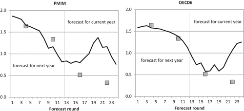
Figure 1 shows exemplarily the time paths of the root-mean-squared forecast errors (RMSFEs) for the forecast of world GDP by the use of these indicators, starting with a forecast from January (1) to December (12) for the growth rate of next year and continuing from January (13) to December (24) with the nowcast for the current year’s growth rate. The corresponding RMSFEs of WEO forecasts are given by the grey quads. For the forecast rounds 1–3 (January–March forecast for GDP growth in the following year), no IMF forecast is available and only indicator forecasts can be used. In general, forecast errors decrease significantly with increasing forecast rounds since the indicators contain more and more information on the real economy. In the months when a new WEO is published, forecasts based on indicators hardly ever beat the WEO, but they do so only a few months later, particularly relative to the October outlook for the next year (t = 10 onwards). Furthermore, Figure 1 also illustrates that indicators are leading the business cycle and that the predictive power for the current year deteriorates at the end of that year.

Figure 1. RMSFE for world GDP forecasts.

Notes: The line shows the RMSFE for indicator forecasts based on PMI manufacturing and OECD+6 composite indicators. The RMSFE for the corresponding WEO forecast is marked by the grey quad. Forecast rounds 1–12 correspond to the forecast for the following year, forecast rounds 13–24 to the current year’s forecast.Source: IMF WEO, April 2016, OECD 2016, and own calculations.

If the forecast errors of the single indicator-based forecasts are compared with the forecast errors of the IMF forecast, it turns out that some indicators might improve the forecast quality significantly in some forecasting rounds.⁷ Table 1 shows the relative forecast performance of the indicator-based forecasts to the most recent IMF forecast (the benchmark) for all country aggregates. Both PMI (manufacturing) and the OECD+6 leading indicator perform quite well up to month 15, and in particular they improve the forecast quality of world GDP compared to IMF WEO forecast up to forecast round 15. Using the PMI manufacturing index for the forecast of the next year and at the beginning of the current year provides substantial improvement. At the end of December, we can improve the forecast for the next year by more than 40%. The OECD+6 indicator increases the forecast performance in the first month of the current year. In general, the improvement of the WEO forecast by the selected indicators is higher for the world aggregate than for the emerging economies or advanced countries. For the latter especially, PMI might improve the forecast up to 20%.

Table 1. Theil’s U for selected indicators.

	World			Emerging			Advanced
	PMIM	OECD6	IP W	OECD6	MSCI EL	IP EL	PMI	MSCI ADV
Forecast for next year
1	NA	NA	NA	NA	NA	NA	NA	NA
2	NA	NA	NA	NA	NA	NA	NA	NA
3	NA	NA	NA	NA	NA	NA	NA	NA
4	0.930	0.962	0.905	1.130	0.944	0.998	1.062	1.087
5	0.910	0.955	0.835	1.117	1.125	1.046	1.051	1.090
6	0.884	0.946	0.906	1.101	1.054	1.053	0.977	1.029
7	0.858*	0.925	0.905	1.080	0.965	1.067	0.949	0.943
8	0.760*	0.906	0.862	1.047	0.993	1.036	0.959	1.032
9	0.633*	0.877	0.835	0.996	0.872	1.089	0.888	1.135
10	0.829	1.036	1.090	1.132	1.161	1.356	1.197	1.068
11	0.697	0.957	0.939	1.060	1.110	1.276	1.033	1.337
12	0.581	0.849	0.933	0.996	1.202	1.192	0.999	1.369
Forecast for current year
13	0.583	0.688	0.674	1.371	1.245	1.227	0.773	1.440
14	0.545	0.547*	0.762	0.977	1.412	1.370	0.762	1.404
15	0.574	0.579	1.149	0.755*	1.466	1.309	0.856*	1.508
16	1.637	1.134	3.197	0.848	2.576	1.476	2.412	5.095
17	1.846	1.149	2.683	0.932	2.649	2.563	2.486	4.707
18	2.055	1.431	3.297	0.981	2.516	2.294	2.951	5.489
19	2.550	1.150	3.119	0.947	2.576	2.774	3.524	4.026
20	2.813	1.311	3.569	1.340	2.400	2.368	3.544	3.887
21	2.353	1.742	3.598	1.535	1.997	2.744	3.363	6.270
22	3.492	3.102	5.077	2.363	3.510	3.742	5.834	8.876
23	2.803	3.547	4.943	2.567	3.013	3.794	6.980	8.299
24	2.283	3.641	4.403	2.562	3.245	3.555	4.726	9.709

Notes: Forecast round 1 corresponds to the first forecast that is made for a year; forecast round 24 is the last forecast round. Forecast rounds 1–12 correspond to the forecast for the following year, forecast rounds 13–24 for the current year’s forecast. IMF forecast releases occur in forecast rounds 4, 10, 16 and 22. Evaluation period 2004–2015. * indicates that the forecast ability is significant at the 10% level.

The OECD+6 leading indicator is not only useful for improving the outlook for the world, but for emerging markets as well, but, remarkably, it does not help to improve the forecast for the advanced countries, although these are the economies the indicator is mainly constructed for. An explanation could be that the information the OECD indicator gives is already incorporated in the IMF forecasts for advanced countries, but the spillovers to the emerging markets are not fully taken into account by the IMF.

In general, the results indicate that for some indicators, a pure indicator-based forecast is better than the IMF only a few months after publication of the WEO.⁸ However, also for these months where the IMF forecast cannot clearly be outperformed by indicator-based forecasts, it might be the case that the indicators contain additional information. Tests of forecast encompassing show that the null cannot be rejected for most of the indicators. However, in line with the results in Table 1, the null can be rejected for the forecast of the next year in the months of October, November and December and for the current year forecast from January to March. Hence, remarkably, there is information in these indicators that is not encompassed by the IMF forecasts even at the time when the IMF forecast is published (which could be related to the publication lag of the WEO).

IV. Conclusions

The study shows that simple indicator-based forecasts perform about equally well as the autumn forecast of the IMF for next year’s output growth at the time the IMF’s outlook is published. Furthermore, they perform better only a few months after the publication, when the indicators contain more recent information. In particular, the IMF’s forecast in October for global economic growth in the following year is significantly outperformed by indicator-based forecasts such as forecasts based on the global manufacturing PMI and the OECD+6 leading indicator. The same is true at the beginning of the current year. Given that forecasting with help of these indicators is quite simple, doing so appears to be a sensible complement to looking at the forecasts published by the IMF. In the light of this result, the IMF was certainly well advised in 2007 to start publishing a regular January (and July) update. However, this is done only for a selection of variables yet. The fact that the OECD indicator is useful in improving IMF forecasts for emerging markets, but not for advanced economies, might tell us that the cyclical connections between advanced and emerging market economies are not yet fully understood and incorporated in the forecasts. However, it should be noted that the results derived in this study are based on a fairly small number of observations and a volatile time period. In particular, the results are, to some extent, driven by the large errors of most forecasts, including those of the IMF, on the eve and during the Great Recession of 2008–2009. Thus, the robustness of the results derived in this article should be reviewed regularly in the next years.

Acknowledgements

We would like to thank Sebastian Giesen for extensive discussion of previous versions of the article. We are grateful to anonymous referees for helpful comments and suggestions.

Disclosure statement

No potential conflict of interest was reported by the authors.

Notes

¹ Besides the two main forecasts in April and October, updates are published in January and July for key national accounts figures and are available electronically since July 2007. Due to the short history, these updates will not be considered in our analysis, although they should be considered for future analyses.

² Note that while Jakaitiene and Dées (2012) use regional aggregates, they do not work with WEO data, and rather use monthly series to be forecasted, such as industrial production, consumer prices, or trade. Golinelli and Parigi (2014) make quarterly forecasts and use own definitions for the group of advanced countries (only six countries) and the group of emerging countries (only the BRICs: Brazil, Russia, India and China). Ho and Mauro (2016) distinguish between low-, middle- and high-income countries.

³ The literature usually deals with the conversion from monthly to quarterly data referring to the average values of months (e.g. Zheng and Rossiter 2006; Armesto, Engemann, Owyang 2010) or they deal with interpolation from lower to higher frequencies (mostly applications of Chow and Lin 1971 method). Mixed-data sampling (MIDAS) methods might also be applied to deal with the mixed-frequency problem (see, e.g., Ferrara and Marsilli 2014, for application with Factor-MIDAS).

⁴ If lagged GDP values are not allowed in the equation, the forecast results are worse.

⁵ The first estimation sample covers from 1992 until 1999. For PMI 1998–2003.

⁶ During the months 1–3, 4–9, and 10–12, the coefficients of the estimated equations remain constant within a year for the indicators that were not revised, e.g. PMI and MSCI.

⁷ Note that if we apply the correction for small sample properties as suggested by Harvey, Leybourne, and Newbold (1997), the differences are no longer significant for neither forecast round.

⁸ The results are in line with Frenkel, Rülke, and Zimmermann (2013) who show that the strategic behaviour of private sector forecasters – using the latest indicator information – lasts roughly 3 months.

References

- Aldenhoff, F.-O. 2007. “Are Economic Forecasts of the International Monetary Fund Polit- Ically Biased? A Public Choice Analysis.” The Review of International Organizations 2 (3): 239–260. doi:10.1007/s11558-006-9010-x.
- Armesto, M. T., K. M. Engemann, M. T. Owyang, et al. (2010): “Forecasting with Mixed Frequencies,” Review 6, Federal Reserve Bank of St. Louis.
- Artis, M. 1996. How Accurate are the IMF’s Short-Term Forecasts?: Another Examination of the World Economic Outlook. Washington D.C: International Monetary Fund.
- Atoyan, R., and P. Conway. 2011. “Projecting Macroeconomic Outcomes: Evidence from the IMF.” The Review of International Organizations 6 (3): 415–441. doi:10.1007/s11558-011-9109-6.
- Chong, Y. Y., and D. F. Hendry. 1986. “Econometric Evaluation of Linear Macro-Economic Models.” The Review of Economic Studies 53 (4): 671–690. doi:10.2307/2297611.
- Chow, G. C., and A.-L. Lin. 1971. “Best Linear Unbiased Interpolation, Distribution, and Extrapolation of Time Series by Related Series.” The Review of Economics and Statistics 53 (4): 372–375. doi:10.2307/1928739.
- Dreher, A., S. Marchesi, and J. Vreeland. 2008. “The Political Economy of IMF Fore- Casts.” Public Choice 137 (1): 145–171. doi:10.1007/s11127-008-9318-6.
- Ferrara, L., and C. Marsilli (2014): “Nowcasting Global Economic Growth: A Factor- Augmented Mixed-Frequency Approach,” Working Paper 515, Banque de France.
- Frenkel, M., J.-C. Rülke, and L. Zimmermann. 2013. “Do Private Sector Forecasters Chase after IMF or OECD Forecasts?” Journal of Macroeconomics 37: 217–229. doi:10.1016/j.jmacro.2013.03.002.
- Genberg, H., and A. Martinez (2014): “On the Accuracy and Efficiency of IMF Forecasts: A Survey and Some Extensions,” Background Paper BP 14/04, Independent Evaluation Office of the International Monetary Fund.
- Giacomini, R., and H. White. 2006. “Tests of Conditional Predictive Ability.” Economet- Rica 74 (6): 1545–1578. doi:10.1111/ecta.2006.74.issue-6.
- Golinelli, R., and G. Parigi. 2014. “Tracking World Trade and GDP in Real Time.” Inter- National Journal of Forecasting 30 (4): 847–862. doi:10.1016/j.ijforecast.2014.01.008.
- Harvey, D., S. Leybourne, and P. Newbold. 1997. “Testing the Equality of Prediction Mean Squared Errors.” International Journal of Forecasting 13 (2): 281–291. doi:10.1016/S0169-2070(96)00719-4.
- Ho, G., and P. Mauro. 2016. “Growth–Now and Forever?” IMF Economic Review 64 (3): 526–547. doi:10.1057/imfer.2016.12.
- Jakaitiene, A., and S. Dées. 2012. “Forecasting the World Economy in the Short Term.” The World Economy 35 (3): 331–350. doi:10.1111/twec.2012.35.issue-3.
- Pons, J. 2000. “The Accuracy of IMF and OECD Forecasts for G7 Countries.” Journal of Forecasting 19 (1): 53–63. doi:10.1002/(ISSN)1099-131X.
- Timmermann, A. 2007. “An Evaluation of the World Economic Outlook Forecasts.” IMF Staff Papers 54 (1): 1–33. doi:10.1057/palgrave.imfsp.9450007.
- West, K. D. 1996. “Inference about Predictive Ability.” Econometrica 64 (5): 1067–1084. doi:10.2307/2171956.
- Zheng, I. Y., and J. Rossiter (2006): “Using Monthly Indicators to Predict Quarterly GDP,” Working Papers 06-26, Bank of Canada.