Poverty risk of the unemployed in six European countries: why is it higher in some countries than in others?

ABSTRACT

In all European countries unemployed persons face a high risk of relative poverty, but poverty rates vary greatly among EU countries. We analyse to what extent these differences could be explained by a different composition of the unemployed or by differences in the national income distribution functions. Our results indicate that the effects of individual characteristics on the poverty risk are roughly comparable between countries, but the composition of the unemployed is very different, which explains on average half of the cross-country differences in poverty rates.

KEYWORDS:

• Poverty
• unemployment
• European union
• income distribution

JEL CLASSIFICATION:

• D31
• I32

I. Introduction

The relative risk of poverty, defined by living below the poverty line of 60% of the median disposable income, is one of the leading social indicators within the European Union. In all countries, unemployed persons face a particularly high risk of relative poverty since they are lacking earned income. However, there is also substantial cross-country heterogeneity. In 2013, the poverty rate of the unemployed amounted to around 70% in Germany, whereas it was below 30% in Denmark and 47% in the EU-28. Several factors contribute to these cross-country differences, e. g. differences in national income protection systems. Apart from redistribution, the structure of households and the distribution of individual characteristics play a major role. The present note provides evidence that differences in the composition of the unemployed can explain to a significant extent cross-country differences in poverty rates of the unemployed.

II. Data and methodology

We use the cross-sectional component of the Scientific Use File (SUF) of EU-SILC 2014 (European Union Statistics on Income and Living Conditions) provided by Eurostat (Eurostat 2013).¹ EU-SILC is based on yearly national representative surveys of private households in the 28 EU member states. We calculate the national poverty threshold as 60% of the median of the equivalized disposable income of the total population, using total disposable income provided in EU-SILC and the modified OECD equivalence scale. In accordance with the Eurostat statistics on poverty and social exclusion, we classify someone as unemployed if (s) he was unemployed for more than six months during the reference year, which is the preceding year (2013).

We focus on six European countries: Belgium (BE), Germany (DE), Spain (ES), Sweden (SE), Slovakia (SK) and the United Kingdom (UK). These countries were selected for two reasons: First, they differ with regard to the poverty risk of the unemployed, with very high (DE, UK), close to the EU-28 average (SK, ES) and low (BE, SE) poverty rates (see Table 1).² Second, the six countries represent a variety of welfare state types, according to the well-known welfare state typology of Esping-Andersen (1990) and later extensions and modifications of this typology.³ Sweden represents the ‘universalist’ social democratic welfare state model, Germany and Belgium stand for the ‘continental’ model, the UK comes close to the ‘liberal’ model, Spain represents the Mediterranean ‘rudimentary’ welfare state type and Slovakia belongs to the heterogeneous group of post-socialist welfare states.

Table 1. Poverty rates by country, 2013.

	BE	DE	ES	SE	SK	UK
Poverty rates (percent):
All	15.3	16.0	21.7	14.8	12.5	16.6
Unemployed	43.2	70.4	47.4	40.2	48.6	56.9
Base household (estimated)	23.8	33.9	36.1	22.4	30.8	36.6
Effect of a change to… on poverty risk of base household (pc. points)
Single	2.1	9.4	17.7	26.6	8.4	29.3
Single Parent	18.9	−4.3	18.2	13.5	12.7	−3.5
≤ 29 years	−1.2	8.9	1.2	2.1	−6.9	−7.4
>49 years	0.2	−2.8	−8.4	−12.2	−3.1	−9.5
High qual.	−6.9	−8.9	−13.5	−0.9	−2.3	−1.8
Low work intensity	33.8	39.9	35.6	31.8	63.5	31.7

Note: Baseline household of a low qualified unemployed aged between 30 and 49 years living in a household with two or more adults and with a high work-intensity.

Source: Own calculation based on EU-SILC 2014

Table 2. Decomposition of cross-country poverty rate-differences.

Countries	P.-rate difference	Difference due to poverty function	Difference due to population structure
BE/DE	−0.30	−0.20	−0.10
BE/ES	−0.07	−0.09	0.02
BE/SE	0.03	−0.03	0.06
BE/SK	−0.05	−0.22	0.17
BE/UK	−0.18	−0.18	0.00
DE/BE	0.30	0.20	0.10
DE/ES	0.23	0.09	0.14
DE/SE	0.33	0.16	0.17
DE/SK	0.24	−0.09	0.34
DE/UK	0.12	0.02	0.09
ES/BE	0.07	0.09	−0.02
ES/DE	−0.23	−0.09	−0.14
ES/SE	0.10	0.09	0.02
ES/SK	0.02	−0.12	0.14
ES/UK	−0.11	−0.06	−0.06
SE/BE	−0.03	0.03	−0.06
SE/DE	−0.33	−0.16	−0.17
SE/ES	−0.10	−0.09	−0.02
SE/SK	−0.09	−0.17	0.09
SE/UK	−0.22	−0.15	−0.07
SK/BE	0.05	0.22	−0.17
SK/DE	−0.24	0.09	−0.34
SK/ES	−0.02	0.12	−0.14
SK/SE	0.09	0.17	−0.09
SK/UK	−0.13	0.04	−0.17
UK/BE	0.18	0.18	−0.00
UK/DE	−0.12	−0.02	−0.09
UK/ES	0.11	0.06	0.06
UK/SE	0.22	0.15	0.07
UK/SK	0.13	−0.04	0.17

Source: Own calculation based on EU-SILC 2014

Our sample comprises 124,680 observations with 7,503 unemployed respondents. We keep only observations with positive household incomes and valid values for the control variables considered in the analysis, which leaves us with 6,830 observations of unemployed individuals.⁴

We built on Biewen and Jenkins (2005) and estimate a parametric specification of the distribution of the net household equivalence income for households with at least one unemployed person for each country, based on a Singh–Maddala (SM) distribution function (Bandourian 2003):

(1) $F_{SM}(y,a,b,q)=1-{\left[\frac{1}{1+\left({\frac{y}{b}}^a\right)}\right]}^q$(1)

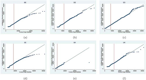
where $a,b,q>0$, $y>0$.⁵ Figure A1 in the Appendix shows a good fit between the sample and the theoretically expected quantiles, especially around the poverty lines (vertical lines), indicated by the closeness of the points to a 45${ }^{\circ }$-line which stands for a perfect fit.

Figure A1. Quantile–quantile-plots for equivalent disposable income of the unemployed.

Source: Own calculation based on EU-SILC 2014

Next, we estimate the distribution models for each country conditional on individual and household characteristics. We choose household composition, the age of the unemployed, education and an indicator for a low work intensity as explanatory variables. Low work intensity means that the working age members in the household worked less than 20% of their potential working time during the reference year. Table A2 in the Appendix shows a large variation of these variables across countries.

Last, we decompose poverty rate differences between two countries $P_1(t_1)$ and $P_2(t_2)$:

(2) $P_1(t_1)-P_2(t_2)=\underset{w}{\int }{F}_1(t_1|{\beta }_1,w)d{G}_1(w)-\underset{w}{\int }{F}_2(t_2|{\beta }_2,w)d{G}_1(w)+\underset{w}{\int }{F}_2(t_2|{\beta }_2,w)d{G}_1(w)-\underset{w}{\int }{F}_2(t_2|{\beta }_2,w)d{G}_2(w),$(2)

or

(3) $P_{11}-P_{22}=[P_{11}-P_{21}]+[P_{21}-P_{22}]$(3)

where the aggregate poverty rate is

(4) $P(t)=\underset{w}{\int }F(t|\beta ,w)dG(w),$(4)

with the poverty function $F(t|\beta ,w)$ of the subpopulation with the characteristics $w$, the poverty line $t$ and the population distribution function $G(w)$. The first difference in Equation (2), $P_{11}-P_{21}$, describes differences in the aggregated poverty rates due to cross-national differences in the poverty functions. The second difference $P_{21}-P_{22}$ describes the difference due to a different composition of the unemployed in both countries. Alternatively, poverty rate differences could be decomposed into these two contributions in a reverse order:

(5) $P_{11}-P_{22}=[P_{11}-P_{12}]+[P_{12}-P_{22}]$(5)

We calculate all components of Equations (3) and (5) for all differences between the six countries, i. e. for 15 country pairs, whereas $G(w)$ is the (weighted) distribution of the characteristics of unemployed below the poverty line in each country. We present the results as weighted average of both approaches shown in Equations (3) and (5) (Biewen and Jenkins 2005):

(6) $\begin{array}{c}{P}_{11}-P_{22}=[0.5((P_{11}-P_{21})+(P_{12}-P_{22}))]\\ +[0.5((P_{21}-P_{22})+(P_{11}-P_{12}))]\end{array}$(6)

III. Estimation results

Table 1 shows in the third row the estimated poverty risk for a reference household. The reference household is a low-qualified unemployed aged between 30 and 49 years, living in a household with two or more adults and with high work intensity. The rows below give the estimation results for the effect of a change of a characteristic on the poverty risk in percentage points, holding the other covariates constant. Living alone or as a lone parent leads to an increase in all countries, with the notable exception of Germany and the UK in the case of single parents. Age has, on the whole, only a moderate influence. A higher skill level is associated with a reduction of poverty rates, as could be expected. The work intensity of the household has by far the strongest effect in all countries. Low work intensity lifts the risk by more than 30 percentage points everywhere, and by even more than 60 percentage points in Slovakia. In Germany, the share of unemployed persons living in households with low work intensity is particularly high (see Table A2), whereas it is lowest in Slovakia. This is closely linked to the respective share of persons living alone, because single-person households mostly have a low work intensity.

The results of the decomposition analysis shown in Table 2 reveal that about half of the cross-country poverty differences are on average due to composition effects. It should be noticed that this result is based on an analysis considering only four, albeit important, characteristics. It is plausible that the proportion explained by differences in the composition increases if further variables could be included.

Furthermore, the results show the variations in the explanation of poverty between countries. The good performance of Belgium (BE) is mainly explained by the contribution of differences in the conditional poverty function. In Germany (DE), the country with the highest poverty risk, the high poverty risk for unemployed is to a significant extent due to an unfavourable population structure. For Spain (ES), the picture is more balanced and Sweden (SE), the country where unemployed face the lowest poverty risk, is characterised by a more favourable distribution of income compared to Germany, Spain, Slovakia and UK. For Slovakia (SK) the results show that differences in poverty rates are mostly explained by an unfavourable income distribution. The UK depicts a middle position, regarding the contribution of the composition and distribution effect.

IV. Conclusion

In this note, we have studied the influence of differences in the composition of the unemployed on differences in the poverty rate of the unemployed between six European countries. We find that most characteristics have the same effect on the poverty risk in all countries, albeit with a different intensity. The results of a decomposition analysis show that about half of the cross-country poverty differences are on average due to observed differences in the composition of the unemployed. Some countries have an advantage in terms of a favourable distribution of poverty-relevant characteristics among the unemployed, but also have a more unfavourable income distribution (Slovakia, partially Spain) or vice versa (Belgium, Sweden, UK). Germany however has both, an unfavourable structure of the unemployed and a high concentration of the unemployed around the poverty line.

Disclosure statement

No potential conflict of interest was reported by the authors.

Notes

¹ The responsibility for all conclusions drawn from the data lies entirely with the authors.

² Denmark, the country with the lowest poverty rate, could not be included because the sample size was too small for our estimations.

³ For a summary of these extensions and modifications, see Seeleib-Kaiser (2008).

⁴ The indicator for the work intensity in the household, one of our control variables, is defined in the EU-SILC only for individuals below 60 years of age.

⁵ For the estimation of the distribution parameters, we use the Stata commands smfit written by Jenkins (2004). Estimation results are shown in Table A3.

Appendix

Table A1. Estimates of SM-distribution parameters by country.

	BE	DE	ES	SE	SK	UK
a	5.2	5.5	2	3.1	2.3	4.2
std. error	.41	.42	.071	.23	.12	.34
b	12418	8554	13180	20349	7116	10458
std. error	584	216	1173	1461	1285	574
q	.67	.58	2.1	1.3	2.6	.72
std. error	.095	.06	.25	.18	.73	.1
Observations	676	847	4175	358	888	486
Clusters	631	775	3236	325	699	440

Source: Own calculation based on EU-SILC 2014

Table A2. Individual and household characteristics of the unemployed (per cent).

	BE	DE	ES	SE	SK	UK
Single	27	45	8	20	5	21
Single Parent	10	9	3	9	1	8
Couple w/o children	29	26	42	28	44	37
Couple w/children	34	20	47	43	50	34
Female	52	48	50	48	51	36
Age ≤29 years	28	16	22	36	33	47
Age >29 years & ≤49 years	47	45	56	41	43	36
Age>49 years	25	40	21	23	24	17
Low qualified	39	31	58	28	21	51
Medium qualified	41	59	20	53	69	30
High qualified	20	11	22	19	10	19
Low work-intensity	56	78	50	42	36	60

Note: Shares in per cent. Source: Own calculation based on EU-SILC 2014

Table A3. Estimates of distribution parameters by country.

Variables	BE	DE	ES	SE	SK	UK
Parameter a
Single	.5057	2.107	.04108	.2202	.6567	1.311
Single Parent	3.01	.9628	.626	.8965	.7847	2.057
Couple	−.4386	.02105	.3483	.7436	.3944	−.51
Age ≤ 29 years	.8567	1.032	.2456	.1787	1.07	1.066
Age > 29 & ≤49 years	1.355	1.159	.325	.3368	.1521	1.285
Age > 49 years	.8655	.8998	.4448	1.345	.6142	.5071
Low Qualified	−.1606	−.4194	.1675	−.1183	.4993	.9269
Low Work Intensity	−.916	−.5788	−.6577	−1.29	−.3815	−1.326
Const.	4.077	4.091	2.015	2.86	2.836	3.857
Parameter b
Single	1453	143.2	1822	857.7	290.6	−184.2
Single Parent	−382	3405	605.8	483.7	1155	1776
Couple	3356	1718	3103	6645	893.3	2548
Age ≤ 29 years	2222	1240	1853	1985	384.3	1778
Age > 29 & ≤49 years	662	1983	1535	4003	1266	315.7
Age > 49 years	1543	2042	2143	1999	688.6	2045
Low Qualified	560.3	368.3	−1393	2501	−193.3	1029
Low Work Intensity	352.8	−3228	−3095	3025	−3324	−16.76
Const.	12620	9362	9627	16179	4387	8235
Parameter q
Single	−.1869	−.3476	.3015	.2405	−.5676	−.01348
Single Parent.	−.1019	.4178	.08553	−.3316	1.887	−.1476
Couple	.08632	−.2151	−.09567	.1719	−.6325	.09344
Age ≤ 29 years	.03035	.03453	.278	.07027	−.2222	.03086
Age > 29 & ≤49 years	−.167	−.03995	.1408	.5869	.7585	−.08997
Age > 49 years	−.06588	−.1394	−.1274	−.5764	.151	−.008578
Low Qualified	.4543	.3318	.6239	.6767	.4021	.168
Low Work Intensity	1.992	.3084	.5866	2.284	−.08667	.9434
Const.	.7975	.8551	1.291	1.081	1.687	.4323

Source: Own calculation based on EU-SILC 2014

References

- Bandourian, R., J. McDonald, and R. Turley. 2003. “A Comparison of Parametric Models of Income Distribution across Countries and over Time.” Estadistica 55: 135–152.
- Biewen, M., and S. Jenkins. 2005. “A Framework for the Decomposition of Poverty Differencees with an Applicatin to Poverty Differences between Countries.” Empirical Economics 30: 331–358. doi:10.1007/s00181-004-0229-1.
- Esping-Andersen, G. 1990. The Three Worlds of Welfare Capitalism. Princeton: Princeton University Press.
- Eurostat. 2013. “EU-SILC 065 (2013 Operation). Description of Target Variables: Cross-Sectional and Longitudinal. 2013 Operation (Version May 2013).” European Commission. Directorate F: Social Statistics and Information Society. https://circabc.europa.eu/sd/a/cacec83d-9db2-4688-80cb-d2a9342eb93c/SILC065%20operation%202012%20VERSION%20MAY%202013.pdf
- Jenkins, S. P. 2004. Fitting Distributions by Maximum Likelihood. Berlin: Presentation at Second German Stata Users Group Meeting.
- Seeleib-Kaiser, M., ed. 2008. Welfare State Transformations. Comparative Perspectives. New York: Palgrave/Macmillan.