Credit spread and employment growth – a time-varying relationship?

ABSTRACT

In this article, I explore time variation in the relationship between the credit spread and employment growth. Using a Bayesian VAR framework and formal model selection, it is concluded that the relationship is best modelled with constant parameters, but that heteroscedasticity needs to be taken into account. An interesting change in the dynamics is uncovered, where volatility in employment shocks induces more of the dynamics earlier in the sample and the role of volatility in credit-spread shocks is more pronounced in the latter parts.

KEYWORDS:

• Bayesian VAR
• time-varying parameters
• stochastic volatility
• macrofinance

JEL CLASSIFICATION:

• E24
• E44
• C32
• C11

I. Introduction

Using financial variables to capture important aspects of macroeconomic relationships is a growing topic in the literature (Chodorow-Reich 2013; Christiano, Motto, and Rostagno 2014; Faust et al. 2013). Recently attention has been paid to the potential of time-variation to such relationships (Aastveit, Natvik, and Sola 2017; Karlsson and Österholm 2020; Xu and de Haan 2018). Including time-variation has an intuitive appeal, not least in the wake of the financial crisis and the ensuing low interest rate/low inflation period (Stock and Watson 2012).

This article tests whether the relationship between the credit spread and employment growth in the United States is time-varying. Theoretically, the interest in credit spreads has been motivated as capturing important financial frictions, particularly the supply of credit to constrained firms (Gilchrist and Zakrajšek 2012). Time variation in the relationship between credit spreads and employment was recently addressed in a paper by Xu and de Haan (2018). In a rolling window regression framework, they concluded that the strength of the relationship has been time-varying. Particularly they find that the variation coincides with periods when quantitative easing was employed and argue that their result reflects that such policies affected the price of risk rather than macroeconomic variables.

The question of how to model time-variation is a debated topic also in the literature on monetary policy (Cogley and Sargent 2005; Korobilis 2013; Nakajima 2011; Primiceri 2005). This article draws on this literature and uses Bayesian VAR models with time-varying parameters, specifically the method of Chan and Eisenstat (2018), to formally assess if the data is best modelled with time-varying parameters and/or stochastic volatility. Contrary to Xu and Haan the results in this article suggest that the relationship is best interpreted as time-invariant. The findings are instead in line with Karlsson and Österholm (2020) who find no time-variation in the relationship between the Baa-spread and GDP growth in the United States. I argue that this difference is largely due to the presence of heteroscedasticity. Time-variation in the R², analysed by Xu and Haan, could be due to time-variation to the volatility of the shocks rather than to the parameters.¹ With this interpretation results are actually similar, but the Bayesian VAR framework lends to a more complete interpretation of the results in terms of relationships and shocks. It is the variance of shocks that is time-varying, not responses to shocks.

This article is structured as follows: Section 2 presents the data and the method, Section 3 presents the empirical analysis and Section 4 concludes.

II. Model and data

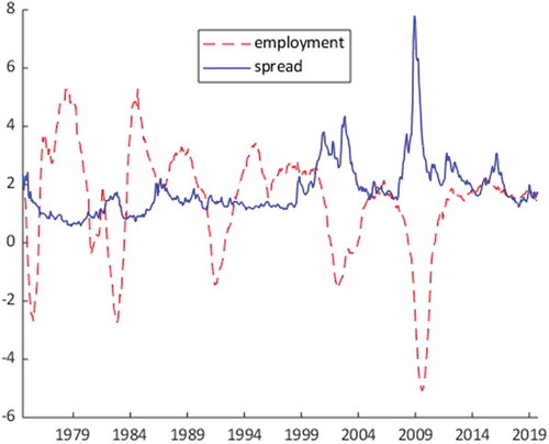
For the credit spread ($G{Z}_t$), I use the updated series provided by Gilchrist and Zakrajšek (2012) for the period January 1973 to September 2019.² A credit spread is the difference between the return on risky and risk-free assets, typically between corporate and government bonds. Since there is often a problem with matching maturities and coupons, Gilchrist and Zakrajšek (2012) calculate the spread using a synthetic government bond. For employment, I use the nonfarm payroll employment.³ Employment growth ($EM{P}_t$) is the year-to-year difference in logged variables (times 100). Time series for the data are presented in Figure 1.

Figure 1. Data

Note: Employment growth in year-on-year per cent change, spread index in percentage points.

Potential time variation in the dynamics is modelled by allowing for time-varying parameters. Stochastic volatility is included to account for heteroscedasticity. Six lags are used. The most general model used is given as

(1) ${\mathit{B}}_{0t}{\mathit{y}}_t={\mu }_t+{\mathit{B}}_{1t}{\mathit{y}}_{t-1}+\dots +{\mathit{B}}_{pt}{\mathit{y}}_{t-p}+{\mathit{\epsilon }}_t$(1)

where $y_t={\left(EM{P}_{t}G{Z}_t\right)}^{\prime }$, ${\mathit{B}}_{0t}$ is a lower triangular matrix with ones at the diagonal, ${\mu }_t$ is the vector of time-varying intercepts, ${\mathit{B}}_{1t},\dots ,{\mathit{B}}_{pt}$ are matrices of time-varying parameters and ${\epsilon }_t$ is a vector of disturbances with ${\epsilon }_t\sim N\left(\mathbf{0},{\mathrm{\Sigma }}_t\right)$ and ${\mathrm{\Sigma }}_t=diag\left(exp\left(h_{1t}\right),exp\left(h_{2t}\right)\right)$. Log volatilities are modelled as random walks

(2) ${\mathit{h}}_t={\mathit{h}}_{t-1}+{\mathit{\varsigma }}_t$(2)

where ${\varsigma }_t\sim \left(0,{\mathrm{\Sigma }}_h\right)$. Also, the free parameters of ${\mathbf{B}}_{it}$ and ${\mu }_t$ are collected into the vector ${\theta }_t$ which is modelled as the random walk process

(3) ${\theta }_t={\theta }_{t-1}+{\eta }_t$(3)

where ${\eta }_t\sim \left(\mathbf{0},{\mathrm{\Sigma }}_{\theta }\right)$. For models with constant regression parameters, there is no variance to the parameters (${\mathrm{\Sigma }}_{\theta }=0$). Homoscedasticity is modelled with constant variance-covariance matrix ${\mathrm{\Sigma }}_t$ (that is, ${\mathrm{\Sigma }}_h=0$).

Following Karlsson and Österholm (2020) priors are chosen to match the scale and variation of the data. A diffuse prior is employed for the initial conditions of the regression parameter vector ${\theta }_0\sim N\left(0,10I\right)$. For models with time-varying parameters, the variance-covariance matrix of Equation (3(3) ${\theta }_t={\theta }_{t-1}+{\eta }_t$(3) ) is a diagonal matrix ${\mathrm{\Sigma }}_{\theta }=diag\left({\sigma }_{\theta i}^2\right)$ with inverse Gamma priors ${\sigma }_{\theta i}^2\sim iG\left({\upsilon }_{\theta i},S_{\theta i}\right)$ with shape parameter ${\upsilon }_{\theta i}=5$ and prior mean of ${\sigma }_{\theta i}^2=0.01$ for the intercept and ${0.01}^2$ for regression parameters.

For models with homoscedasticity, an inverse Gamma prior is set on the diagonal elements of ${\mathrm{\Sigma }}_t$, ${\sigma }_i^2\sim iG\left({\upsilon }_i,S_i\right)$, with ${\upsilon }_i=5$ and a prior mean matching the residual variance of a univariate AR-model with the same lag length as the VAR.

For models with stochastic volatility, a normal prior is specified for the initial conditions $h_0\sim N\left({\mu }_h,0.25I\right)$. Elements of ${\mu }_h$ are chosen such that the prior mean of $\mathrm{e}\mathrm{x}\mathrm{p}\left(h_{i0}\right)$ coincides with the homoscedastic specification. Finally, the variance-covariance matrix of Equation (2(2) ${\mathit{h}}_t={\mathit{h}}_{t-1}+{\mathit{\varsigma }}_t$(2) ) is diagonal with inverse gamma prior on the diagonal elements with ${\upsilon }_{hi}=5$ and mean ${\sigma }_{hi}^2=0.01$ in the models with stochastic volatility. For posterior inference, I use the MCMC sampler of Chan and Eisenstat (2018).

III. Empirical analysis

In this article, I employ Chan and Eisenstat (2018) method to find marginal likelihoods for VARs with time-varying parameters and/or stochastic volatility. Specifically, I look at the following four specifications:

1. Constant ${\theta }_t$, constant ${\mathrm{\Sigma }}_{\mathbf{t}}$

2. Constant ${\theta }_t$, time-varying ${\mathrm{\Sigma }}_{\mathbf{t}}$

3. Time-varying ${\theta }_t$, constant ${\mathrm{\Sigma }}_t$

4. Time-varying ${\theta }_t$, time-varying ${\mathrm{\Sigma }}_{\mathbf{t}}$

Formal Bayesian model selection is then employed based on the (log) marginal likelihoods which are presented in Table 1. The model preferred by the data is the one with stochastic volatility but constant parameters (ii). Throughout, model selection clearly favours models with stochastic volatility.⁴

Table 1. Log marginal likelihood for specifications i to iv.

Model	Log marginal likelihood
i	136.5
ii	413.1
iii	221.3
iv	341.1

Note: The highest log marginal likelihood is marked using bold font

Studying the impulse responses, the response of employment growth to a shock to the spread in the preferred model (ii) has the expected shape (Figure 2). If there is a positive shock to the spread, employment growth decreases. The impulse response function also shows us that the responses peak after 1 to 2 years. Similarly, the response of the spread to an employment-growth shock has an intuitive shape (Figure 3).

Figure 2. Response of employment growth to shocks to credit spread

Note: Size of impulse is one standard deviation. Effect in percentage points on vertical axis, dates on horizontal axis and months on horizon.

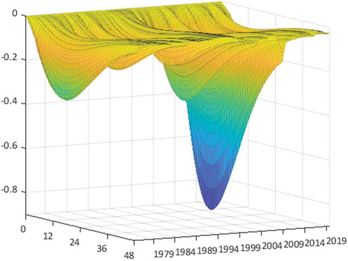
Figure 3. Response of credit spread to shocks to employment growth

Note: Size of impulse is one standard deviation. Effect in percentage points on vertical axis, dates on horizontal axis and months on horizon.

For a more intuitive interpretation of the strengths of the relationships, it could be informative to study the variance decompositions, which depict the share of the forecast error variance explained by shocks to the two variables. Of course, given the model used, time-variation in these must be interpreted in terms of the size of the shocks and not as time-varying parameters (${\theta }_t$). The financial crisis is, for example, modelled as a major shock to the credit spread.⁵ This could be reasonable considering that the credit spread is sometimes described as capturing the appetite for risk, which presumably took a hit following the crisis.

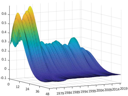
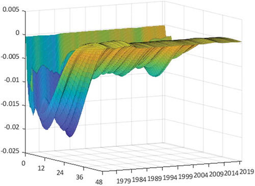
One thing to note is that the shares explained by the different shocks vary considerably over time. During the financial crisis, the credit spread explains as much as about 90% of the variation in the forecast error of employment growth after 1 year (Figure 4). At other times it explains virtually nothing. Interestingly, shocks to employment growth explain a small – but not always negligible – share of the forecast error of the spread early in the sample (Figure 5).

Figure 4. Share of forecast error variance of employment growth explained by shocks to credit spread

Note: Share of forecast error variance explained on vertical axis, dates on horizontal axis and months on horizon.

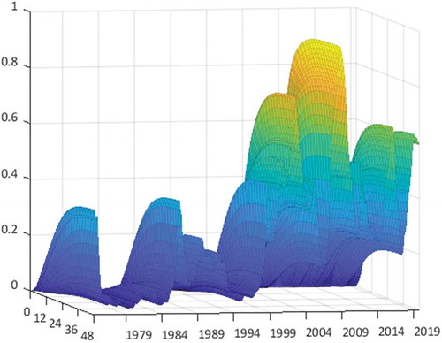
Figure 5. Share of forecast error variance of credit spread explained by shocks to employment growth

Note: See Figure 4.

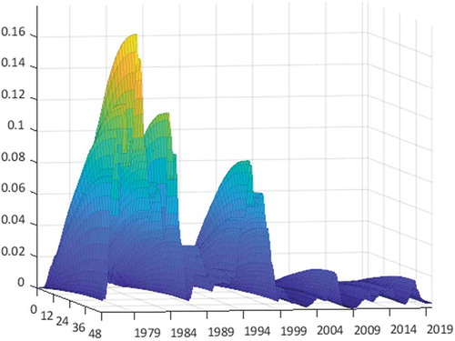
After the mid-1990s, the importance of shocks to employment growth appears to have been reduced, while the importance of shocks to the credit spread appears to have increased. Since this is due to heteroscedasticity it is the characteristics of shocks that have changed. It could be that shocks to the variables in the model have changed, possibly due to the increasing importance of financial markets. Alternatively, it could be that the variables in the model respond differently to variables and shocks not modelled. For example, decreasing regulation and increasing transparency might have made credit spreads more responsive to monetary policy, thus enabling it to anticipate shifts in employment. This relates to a growing literature studying the type of shocks that hit the economy (Bloom 2009; Caldara et al. 2016; Stock and Watson 2012) and a debate on causes of variation to responses to monetary policy shocks (Cogley and Sargent 2001; Sims and Zha 2006).

IV. Conclusion

This article studies the dynamic relationship between credit spreads and employment, focusing on potential time variation. Results suggest that the dynamics are best modelled with constant parameters but that shock volatility is time-varying. A variance decomposition of the preferred model suggests that credit-spread shocks can explain much of the variation in the forecast error of employment growth after the mid-1990s and particularly during the financial crisis.

The variance decomposition calls attention to how heteroscedasticity causes time-variation in the strength of relationships, a change that would materialize as changing R² in a rolling window analysis. Though my analysis does not typically attribute as much explanatory power to the credit spread as Xu and de Haan (2018), and I formulate the opposite interpretation, the actual content of our analyses is not dissimilar. The strength of the relationship has been time-varying. I only add that this is due to changes in the volatility of shocks and not to changes in how employment responds to the credit spread. Such a distinction could be important both for modelling and when designing policy.

Acknowledgments

I am grateful to Pär Österholm for valuable comments and Joshua Chan and Sune Karlsson for sharing code.

Disclosure statement

No potential conflict of interest was reported by the author.

Notes

¹ Ignoring time variation in the volatility of shocks can lead to erroneous conclusions regarding time variation in dynamics as pointed out by Stock (2001).

² Sourced from Macrobond.

³ Sourced from the Federal Reserve Bank of St. Louis.

⁴ Time-variation could also be modelled as discrete. Analysis of a model based on the most general specification in Sims and Zha (2006) (using the specification in Chan and Eisenstat (2018) and priors as specified before) gives a log marginal likelihood of 253.9 when the model has two regimes. A model with three regimes gives a log marginal likelihood of 239.8.

⁵ The variation in shocks is found in Figures A1 and A2 in the Appendix. They are also illustrated in the zero horizons in the impulse response functions on the own variable, see Figures A3 and A4.

Appendix

Figure A1. Standard deviation of shocks to credit spread

Note: Time on horizontal axis and standard deviation of the shocks on vertical, 68% credible interval shaded.

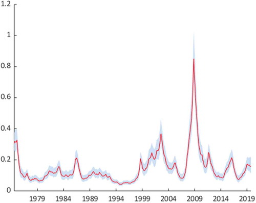
Figure A2. Standard deviation to shocks to employment growth

Note: Time on horizontal axis and standard deviation of the shocks on vertical, 68% credible interval shaded.

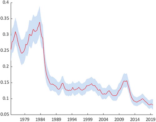
Figure A3. Response of credit spread to shocks to credit spread

Note: See Figure 2.

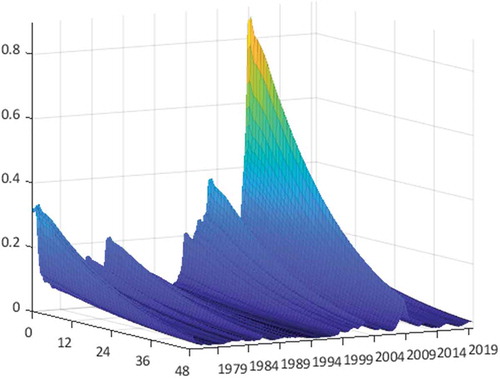
Figure A4. Response of employment growth to shocks to employment growth

Note: See Figure 3.

References

- Aastveit, K. A., G. J. Natvik, and S. Sola. 2017. “Economic Uncertainty and the Influence of Monetary Policy.” Journal of International Money and Finance 76: 50–67. doi:10.1016/j.jimonfin.2017.05.003.
- Bloom, N. 2009. “The Impact of Uncertainty Shocks.” Econometrica 77 (3): 623–685.
- Caldara, D., C. Fuentes-Albero, S. Gilchrist, and E. Zakrajšek. 2016. “The Macroeconomic Impact of Financial and Uncertainty Shocks.” European Economic Review 88: 185–207. doi:10.1016/j.euroecorev.2016.02.020.
- Chan, J. C., and E. Eisenstat. 2018. “Bayesian Model Comparison for Time‐varying Parameter VARs with Stochastic Volatility.” Journal of Applied Econometrics 33 (4): 509–532. doi:10.1002/jae.2617.
- Chodorow-Reich, G. 2013. “The Employment Effects of Credit Market Disruptions: Firm-level Evidence from the 2008–9 Financial Crisis.” The Quarterly Journal of Economics 129 (1): 1–59. doi:10.1093/qje/qjt031.
- Christiano, L. J., R. Motto, and M. Rostagno. 2014. “Risk Shocks.” American Economic Review 104 (1): 27–65. doi:10.1257/aer.104.1.27.
- Cogley, T., and T. J. Sargent. 2001. “Evolving Post-world War II US Inflation Dynamics.” NBER Macroeconomics Annual 16: 331–373. doi:10.1086/654451.
- Cogley, T., and T. J. Sargent. 2005. “Drifts and Volatilities: Monetary Policies and Outcomes in the Post WWII US.” Review of Economic Dynamics 8 (2): 262–302. doi:10.1016/j.red.2004.10.009.
- Faust, J., S. Gilchrist, J. H. Wright, and E. Zakrajšsek. 2013. “Credit Spreads as Predictors of Real-time Economic Activity: A Bayesian Model-averaging Approach.” Review of Economics and Statistics 95 (5): 1501–1519. doi:10.1162/REST_a_00376.
- Gilchrist, S., and E. Zakrajšek. 2012. “Credit Spreads and Business Cycle Fluctuations.” American Economic Review 102 (4): 1692–1720. doi:10.1257/aer.102.4.1692.
- Karlsson, S., and P. Österholm. 2020. “The Relation between the Corporate Bond-yield Spread and the Real Economy: Stable or Time-varying?” Economics Letters 186: 108883.
- Korobilis, D. 2013. “Assessing the Transmission of Monetary Policy Using Time‐varying Parameter Dynamic Factor Models.” Oxford Bulletin of Economics and Statistics 75 (2): 157–179. doi:10.1111/obes.2013.75.issue-2.
- Nakajima, J. 2011. “Time-Varying Parameter VAR Model with Stochastic Volatility: An Overview of Methodology and Empirical Applications.” Monetary and Economic Studies 29: 107–142.
- Primiceri, G. E. 2005. “Time Varying Structural Vector Autoregressions and Monetary Policy.” Review of Economic Studies 72 (3): 821–852. doi:10.1111/j.1467-937X.2005.00353.x.
- Sims, C. A., and T. Zha. 2006. “Were There Regime Switches in US Monetary Policy?” American Economic Review 96 (1): 54–81. doi:10.1257/000282806776157678.
- Stock, J. H. 2001. “Comment on Sargent and Cogley’s ‘Evolving US Postwar Inflation Dynamics’.” NBER Macroeconomics Annual 16: 379–387. doi:10.1086/654453.
- Stock, J. H., and M. W. Watson. 2012. “Disentangling the Channels of the 2007–09 Recession.” Brookings Papers on Economic Activity 2012 (1): 81–135. doi:10.1353/eca.2012.0005.
- Xu, Y., and J. de Haan. 2018. “The Time-varying Relationship between Credit Spreads and Employment Growth.” Applied Economics 50 (41): 4387–4401. doi:10.1080/00036846.2018.1450483.