Inclusion of older annual data into time series models for recent quarterly data

ABSTRACT

This note proposes time series models for data where the frequency changes over time. As an example, for many countries, in the past, real GDP growth was observed annually and since a few years or decades, the data are available per quarter. Modifying the time series models allows for the incorporation of these older annual data, without a need for imputation. Illustrations for real GDP growth in China and the Netherlands show the merits of the method.

KEYWORDS:

• Mixed frequency
• time series models
• autoregression
• real GDP growth

JEL CLASSIFICATION:

• C22
• C51

I. Introduction

For many countries, national statistics institutes collect reliable quarterly data for real Gross Domestic Product (GDP) growth, whereas before they used to collect those data only at the annual level. For example, quarterly real GDP growth in China is made available since 1992Q1 by the National Bureau of Statistics of China (NBSC) (www.stats.gov.cn), while annual real GDP growth rates are available from the World Bank since 1961. Statistics Netherlands makes available their real GDP growth rates per quarter through https://opendata.cbs.nl/statline/, where at the time of writing this paper, the available data start in 1995Q1, whereas the World Bank published annual real GDP growth rates again since 1961.

Figure 1 presents the quarterly and annual data for China, starting in 1961 and ending in 2009Q4, see Franses and Mees (2013) for an analysis. It is the purpose of this note to propose a model for the annual and quarterly data at the same time,¹ that is, to account for the gaps in the quarterly data before 1992Q1. The nominal GDP data in current prices data in China are reported in a format that differs from many other countries but is convenient for the present purposes. That is, NBSC presents the data in cumulated format. Writing GDP in quarter Q in year T as $Z_{Q,T}$, then the nominal GDP data look like

$X_{1,T}=Z_{1,T}$

$X_{2,T}=Z_{1,T}^r+Z_{2,T}$

$X_{3,T}=Z_{1,T}^{rr}+Z_{2,T}^r+Z_{3,T}$

$X_{4,T}=Z_{1,T}^{rrr}+Z_{2,T}^{rr}+Z_{3,T}^r+Z_{4,T}$

Figure 1. Quarterly and annual real DGP growth for China, starting in 1961 and ending in 2009Q4

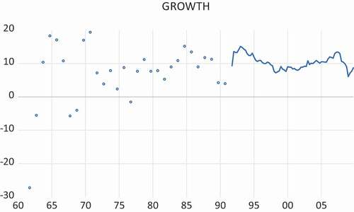
where ‘r’ means the first revision, ‘rr’ the second revision and ‘rrr’ the third revision. The way the data are compiled in the fourth quarter matches with annual GDP. As a consequence, writing $X_T$as total annual GDP, it is clear that

$100\left(log{X}_T-log{X}_{T-1}\right)=100\left(log{X}_{4,T}-log{X}_{4,T-1}\right)$

In other words, the annual data in the years before 1992 for China match with the annual growth rates per quarter, but then only observed in the fourth quarter. In turn, this means that the annual data before 1992 can be treated as quarterly rates with gaps for the quarters Q1, Q2 and Q3, see again Figure 1.

In Section 2 this paper continues with analysing a first-order autoregression for the quarterly GDP growth dates in China. Section 3 focuses on a second-order autoregression for the quarterly data for the Netherlands, which first have to be turned in the cumulated format like in China. Section 4 concludes with various further research topics.

II. Real GDP growth in China: autoregression of order 1

This section will focus on a first-order autoregression and its formulation in case of gaps in the data. The intention is not to impute newly created data in these gaps, but merely to adjust the expression of the model to accommodate the gaps.

Assume there are quarterly real GDP growth figures, based on quarterly cumulative levels data $x_t$, and continue with

$y_t=100(log{x}_t-log{x}_{t-4})$

It is convenient to write a first autoregression as

(1) $y_t-\delta ={\alpha }_1\left(y_{t-1}-\delta \right)+{\epsilon }_t$(1)

where $\delta$ is the mean of the variable and where ${\epsilon }_t$ is a zero mean white noise process with variance ${\sigma }^2$. When this model is fitted to the Chinese data for 1992Q1 to 2009Q4, there are no signs of significant residual autocorrelation, so this autoregression seems to fit the Chinese data well.

Backward substitution of the model in (1) towards $y_{t-4}$ results in

(2) $y_t-\delta ={\alpha }_1^4\left(y_{t-4}-\delta \right)+{\epsilon }_t+{\alpha }_1{\epsilon }_{t-1}+{\alpha }_1^2{\epsilon }_{t-2}+{\alpha }_1^3{\epsilon }_{t-3}$(2)

This shows that skip-sampling the data with frequency 4 does not introduce additional autocorrelation, that is, ${\epsilon }_t+{\alpha }_1{\epsilon }_{t-1}+{\alpha }_1^2{\epsilon }_{t-2}+{\alpha }_1^3{\epsilon }_{t-3}$ is uncorrelated with ${\epsilon }_{t-4}+{\alpha }_1{\epsilon }_{t-5}+{\alpha }_1^2{\epsilon }_{t-6}+{\alpha }_1^3{\epsilon }_{t-7}$. The variance of the error term in the part of the sample that involves the annual data is however larger than ${\sigma }^2$ as it is ${\sigma }^2\left(1+{\alpha }_1^2+{\alpha }_1^4+{\alpha }_1^6\right)$. One may now want to make use of this explicit expression, but one can also resort to the (Newey and West) HAC estimator for the standard errors of the parameters.

Defining a variable $la{g}_t$ which takes a value of 4 until 1992Q1 and of 1 afterwards, the expressions in (1) and (2) can be combined into

(3) $\left(y_t-\delta \right)={\alpha }_1^{la{g}_t}\left(y_{t-la{g}_t}-\delta \right)+u_t$(3)

where $u_t$ is a zero mean white noise process with time-varying variance.

Fitting model (3) using the Generalized Method of Moments (GMM) (performed in EViews version 11), the estimation results for the sample 1962Q4 to 2009Q4 (102 effective observations) are

$\hat{\delta }=9.088\left(1.279\right)$

${\hat{\alpha }}_1=0.765\left(0.045\right)$

where HAC corrected standard errors are given in parentheses. The Ordinary Least Squares (OLS) based estimate of the standard error would have been 0.035, so indeed the HAC correction takes care of the larger variance in the first part of the sample as the HAC standard error exceeds the OLS standard error.

When model (1) is fitted to the effective sample 1992Q2 to 2009Q4, the following estimation results are obtained:

$\hat{\delta }=9.586\left(1.205\right)$

${\hat{\alpha }}_1=0.918\left(0.044\right)$

where now the OLS-based standard errors are reported in parentheses. Comparing the two sets of estimates, it can be seen that the mean growth rate is about the same across the two samples, but the estimates for the first autoregressive parameter differ substantially. In fact, a Dicky Fuller test statistic for the shorter sample is (0.918–1)/0.044 = −1.864, which suggests the presence of a unit root, while the same statistic for the full sample is (0.765–1)/0.045 = −5.222, which suggests a clear rejection of the unit root null hypothesis.²

Hence, one can now conclude that the longer sample introduces more power to a unit root test. However, looking again at the data in Figure 1, it may be that the observation in 1961Q4 is influential as it is large and negative. Re-estimating model (3) for the sample 1963Q4 to 2009Q4 (now with 101 effective observations) gives

$\hat{\delta }=9.164\left(1.182\right)$

${\hat{\alpha }}_1=0.733\left(0.093\right)$

and clearly the HAC-based estimate of the standard error for ${\alpha }_1$ almost doubles. The Dicky-Fuller unit root test value now becomes (0.733–1)/0.093 = −2.871, which is close to the 5% critical value. Hence, one still would conclude here that, based on the full sample, the unit root null hypothesis gets rejected.

III. Real GDP growth in the Netherlands: autoregression of order 2

In this section the focus is on real GDP data for the Netherlands. A graph of the (non-cumulated) real GDP data for 1995Q1 to 2019Q4 is presented in Figure 2. The cumulated levels of real GDP data appear in Figure 3. Figure 4 presents the annual growth rates when observed quarterly, based on not cumulated and cumulated data. It is clear that the two series do not differ much. Finally, Figure 5 adds the annual data observed in the fourth quarter, starting from 1961 onwards.

Figure 2. Real Gross Domestic Product 1995Q1-2019Q4 for the Netherlands (in billions of Euros)

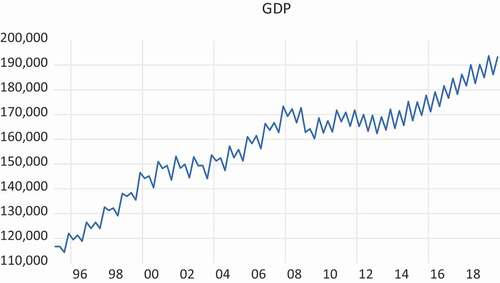
Figure 3. Real Gross Domestic Product 1995Q1-2019Q4 for the Netherlands (in billions of Euros), when cumulated as Q1, Q1+ Q2, Q1+ Q2+ Q3 and Q1+ Q2+ Q3+ Q4

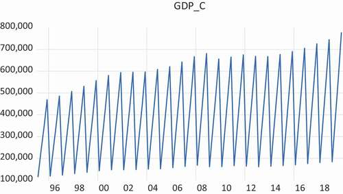
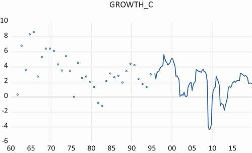
Figure 4. Annual growth rates of Real GDP, 1996Q1-2019Q4, for the Netherlands, based on quarterly GDP figures (GROWTH) and based on cumulative quarterly GDP figures (GROWTH_C), computed as $y_t=100\left(log{x}_t-log{x}_{t-4}\right)$

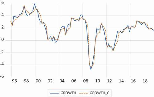
Figure 5. Annual growth rates of real GDP for 1961Q4-2019Q4 for the Netherlands

An analysis of the autocorrelation function of real GDP growth for the last part of the sample involving the actual quarterly data indicates that an autoregression of order 2 describes the data well. To allow for simple backward substitution, as is done in (2), it is convenient to write the second-order autoregression as

$\left(y_t-\delta \right)-{\alpha }_1\left(y_{t-1}-\delta \right)={\alpha }_2\left((y_{t-1}-\delta \right)-{\alpha }_1\left(y_{t-2}-\delta \right))+{\epsilon }_t.$

.

Re-arranging terms gives

$y_t=\delta \left(1-{\alpha }_1\right)\left(1-{\alpha }_2\right)+\left({\alpha }_1+{\alpha }_2\right)y_{t-1}-{\alpha }_1{\alpha }_2{y}_{t-2}+{\epsilon }_t$

and this allows to compute the residuals. Again, the parameters can be estimated using GMM. Backward substitution gives

$\left(y_t-\delta \right)-{\alpha }_1^4\left(y_{t-4}-\delta \right)={\alpha }_2^4\left((y_{t-4}-\delta \right)-{\alpha }_1^4\left(y_{t-8}-\delta \right))+u_t$

where $u_t$ is a zero mean white noise process with time-varying variance. More generally, if $la{g}_t$ is variable that takes a value 4 until 1996.1 and 1 afterwards, then the general form of this second-order autoregression is

$\left(y_t-\delta \right)-{\alpha }_1^{la{g}_t}\left(y_{t-la{g}_t}-\delta \right)={\alpha }_2^{la{g}_t}\left(\left(y_{t-la{g}_t}-\delta \right)-{\alpha }_1^{la{g}_t}\left(y_{t-2la{g}_t}-\delta \right)\right)+u_t$

where $u_t$ still is a zero mean white noise process with time-varying variance.

The estimation results for the sample for the Netherlands that starts in 1963.4 (and has 128 effective observations) are

$\hat{\delta }=3.070\left(0.608\right)$

${\hat{\alpha }}_1=0.854\left(0.059\right)$

${\hat{\alpha }}_2=0.276\left(0.093\right)$

with the HAC corrected standard errors in parentheses. Clearly, all parameters differ from zero, significantly. The Dicky Fuller test value is (0.854–1)/0.059 = −2.475, which is close to the 10% critical value.

The estimation results for the effective sample 1996Q3 to 2019Q4 (94 observations) are

$\hat{\delta }=1.892\left(0.689\right)$

${\hat{\alpha }}_1=0.797\left(0.099\right)$

${\hat{\alpha }}_2=0.334\left(0.156\right)$

where again, now the OLS-based estimated standard errors are in parentheses. The Dicky Fuller test value is (0.797–1)/0.099 = −2.051, which is much further away from the 10% critical value. Hence, also here, one can see that including past annual data provides more evidence against the null hypothesis of a unit root.

IV. Conclusion

This paper has proposed a simple method to include past annual data into models for currently available quarterly data. Application to real GDP growth per quarter for China and the Netherlands showed that the method is easy to apply. As there are longer spans of data to analyse, it was also found that there was more evidence against the unit root null hypothesis.

The method can easily be applied to any type of time series and for any frequency. So, if data are available now at the monthly level and before at the quarterly level, the same tools can be used. Note that it is important to write the model such that there is a multiplication of first-order autoregressive terms in order to make the representation easy to handle.

A next step can be to consider vector autoregressive models and autoregressive distributed lag models for data with similar features.

Disclosure statement

No potential conflict of interest was reported by the author.

Notes

¹ In a sense, my approach mimics a MIDAS model, where two or more variables observed at different frequencies are correlated, see Breitung and Roling (2015), Clements and Galvão (2008), and Ghysels, Santa-Clara, and Valkanov (2004) for useful references. In the present paper, however, the focus is on mixed frequencies over time, and not across variables.

² For the case of an intercept and no trend, the 5% critical value of the Dicky-Fuller test for 100 observations is −2.89, and the 10% critical value is −2.58.

References

- Breitung, J., and C. Roling. 2015. “Forecasting Inflation Rates Using Daily Data: A Nonparametric MIDAS Approach.” Journal of Forecasting 34 (7): 588–603. doi:https://doi.org/10.1002/for.2361.
- Clements, M. P., and A. B. Galvão. 2008. “Macroeconomic Forecasting with Mixed-frequency Data: Forecasting Output Growth in the United States.” Journal of Business & Economic Statistics 26 (4): 546–554. doi:https://doi.org/10.1198/073500108000000015.
- Franses, P. H., and H. Mees. 2013. “Approximating the DGP of China’s Quarterly GDP.” Applied Economics 45 (24): 3469–3472. doi:https://doi.org/10.1080/00036846.2012.709604.
- Ghysels, E., P. Santa-Clara, and R. Valkanov. 2004. “The MIDAS touch: mixed data sampling regression models.” CIRANO Working paper.