How do world commodity prices affect Asian commodity exporting economies? The role of financial frictions

ABSTRACT

This note examines how recent volatile fluctuations of world commodity prices due to the COVID-19 shock affect Asian commodity exporting economies. Our analysis shows that a drop in world commodity prices has a significant negative impact on output, consumption, and investment of sample countries. However, the impact on trade balance is positive in some countries and negative in others. The difference between these two groups is attributable to whether world commodity prices affect each country’s interest rate spreads.

KEYWORDS:

• Commodity prices
• Asian emerging economies
• financial frictions
• SVAR
• COVID-19 shock

JEL CLASSIFICATION:

• E32
• E37
• E44
• F32
• F36
• F41
• F44
• F62
• O16
• Q43

I. Introduction

According to Hevia and Neumeyer (2020), emerging economies are affected by the COVID-19 pandemic through three main channels: (i) the direct negative effect of social distancing restrictions on economic activity, (ii) terms of trade deterioration, and (iii) global financial shock. The first channel involves restrictions on economic activity in many industries, such as travel and entertainment. The second channel is through a sizable output loss due to terms of trade deterioration for commodity-exporting countries. Commodity-exporting countries are experiencing a sharp fall in the commodity prices of their exports due to a decline in global demand. As for the third channel, a global liquidity shock has entailed massive portfolio shifts from riskier assets to safer, liquid assets. For emerging economies, this implies an increase in their risk spreads, capital flow reversals, and the depreciation of their currencies.

This study analyzes the second above-mentioned channel through terms of trade deterioration for commodity-exporting countries. While many previous studies focus on commodity exporting economies in regions like Latin America, we focus on five Asian commodity-exporting economies (Azerbaijan, Indonesia, Kazakhstan, Malaysia, and Mongolia).¹ We show that world commodity price shocks may have significant impacts on Asian commodity exporting economies. We identify world commodity price shocks using a structural vector auto-regression (SVAR) model with a standard Cholesky decomposition. The data from the sample countries reveal that the recent drop in world commodity prices may have significant negative impacts on output, consumption, and investment. Regarding trade balance, we find that the sample countries are divided into two groups: Malaysia, Mongolia, and Indonesia may have positive trade balances, whereas Azerbaijan and Kazakhstan may have negative trade balances. The differences between these two groups in the results of our analysis can be attributed to the effect of world commodity prices on each country’s interest rate spreads. In Malaysia, Mongolia, and Indonesia, a fall in world commodity prices raises interest rate spreads, which leads to a decline in their foreign borrowing, i.e. positive trade balances. On the other hand, in Azerbaijan and Kazakhstan, the effect of world commodity price changes is neutral on their interest rate spreads. This implies that in these countries, the effect of a world commodity price fall is straightforward, as shown in many standard textbooks on open economy macroeconomics. A temporary fall in their exporting commodity prices corresponds to a temporary negative output shock that should be financed by an increase in foreign borrowing, which is achieved by negative trade balances.

Existing evidence from the literature indicates that the existence of a relationship between commodity prices and interest rate spreads is key to identifying the cause of the different results between these two groups regarding trade balance. First, why do world commodity prices affect interest rate spreads in commodity exporting economies. Drechsel and Tenreyro (2018) argue that ‘[t]his could come in the form of a borrowing constraint, in which the value of the country’s collateral depends directly on commodity prices through export earnings (lines 15–18, 206).’ That is, when commodity prices decrease, creditors increase the required interest rate spread because the value of the country’s collateral deteriorates. Following the logic of Drechsel and Tenreyro (2018), we estimate the relationship between interest rate spreads in these economies and world commodity prices by regressing interest rate spreads in these economies on the international commodity price index. We find negative relationships between interest rate spreads and world commodity prices in Malaysia, Mongolia, and Indonesia. In other words, in these countries, a drop in world commodity prices is associated with a rise in interest rate spreads. However, we do not find any significant relationships between the two in Azerbaijan and Kazakhstan. The results of our analysis imply that financial frictions play a role in Malaysia, Mongolia, and Indonesia, but not in Azerbaijan and Kazakhstan.

The remainder of the note proceeds as follows. Section 2 examines the effects of commodity prices on the macroeconomic variables of the five Asian commodity-exporting economies using SVAR. Section 3 examines the relationship between world commodity prices and each country’s interest rate spread using regression analyses. We present our conclusions in Section 4.

II. The effects of world commodity prices on macroeconomic variables

In this study, we choose Azerbaijan, Indonesia, Kazakhstan, Malaysia, and Mongolia as our sample countries following ADB (2016).² We first construct trade-weighted commodity-price indices that each country faces as follows.

Although these countries are all so-called commodity-exporting countries, their baskets of commodity export products, of course, consist of different products with different shares. Therefore, we must construct a country-specific commodity index that each country faces. To construct a country-specific commodity index, we need to determine the prices and weights of commodity exports for each country.

For the export price data, we use the World Bank commodity price data (‘pink sheet’).³ Specifically, we use the commodity price indices for four groups, ‘fuel,’ ‘food,’ ‘raw materials,’ and ‘metal&minerals,’ in the pink sheet. These nominal commodity indices are deflated using the US CPI series.^4,5

For the export weight data, we use the World Integrated Trade Solution (WITS) database.⁶ We obtain the country-specific weights of commodity export products for each country using commodity export product groups defined in terms of the Standard SITC Revision 2 Product Groups. For a given country, we calculate the average share of exports of the corresponding four groups during the sample period.

By applying the country-specific commodity-export weights for the four groups to the corresponding commodity-price indices, we obtain the trade-weighted commodity price index for each country.

In order to estimate the effect of international commodity prices on Asian exporting countries’ business cycles, we consider the following structural vector autoregression (SVAR) for each country:

(1) $A{y}_t=A_1{y}_{t-1}+A_2{y}_{t-2}+\cdots +A_p{y}_{t-p}+Ct+B_{{\in }_t},$(1)

where $y_t$ is a vector of five key variables (i.e. the trade-weighted commodity price index, output, consumption, investment, and the trade-balance ratio to output). We estimate the VAR in levels since it yields consistent estimates even when each variable is not stationary.⁷ The key business cycle variables (output, consumption, investment, and the trade-balance ratio to output) are obtained from International Financial Statistics. The raw series are seasonally adjusted and transformed into real terms using GDP deflator.⁸ Taking logs (except for the trade-weighted commodity price index and the trade-balance ratio to output) and applying the Hodrick–Prescott filter with a smoothing parameter of $1600$, we obtain cycle components for each series.

In Equation (1)(1) $A{y}_t=A_1{y}_{t-1}+A_2{y}_{t-2}+\cdots +A_p{y}_{t-p}+Ct+B_{{\in }_t},$(1) , $A$ is $5\times 5$ matrix of structural coefficients, which represents the contemporaneous relationship among the variables in $y_t$. $A_i(i=1,2,\cdots p)$ is $5\times 5$ matrix of the structural parameters on the lagged endogenous variables. $B$ is $5\times 5$ matrix of coefficients on structural shocks where${\in }_t\sim (0,I_5)$. $C$ is $5\times 1$ matrix of coefficients on a linear time trend.

Since the five Asian commodity-exporting economies are small countries, we assume that domestic variables of the sample countries do not contemporaneously affect world commodity prices. We are therefore able to identify the world commodity price shock by ordering the trade-weighted commodity price index first in a Cholesky decomposition.⁹

Depending on availability, we choose the sample period for each country. The sample period for each country is 2001Q1–2016Q4 for Azerbaijan, 1997Q1–2018Q3 for Indonesia, 2005Q1–2018Q3 for Mongolia, 1991Q1–2018Q4 for Malaysia, and 1994Q1–2015Q4 for Kazakhstan.

The impulse response functions to a one-standard-deviation negative shock of commodity prices are plotted in Figure 1. The first column of Figure 1 shows the impulse responses of output (GDP) in the five countries: Malaysia (MAL), Mongolia (MON), Indonesia (IND), Azerbaijan (AZE), and Kazakhstan (KAZ). The second column shows the impulse responses of consumption (CON) in the five countries. The third column shows the impulse responses of investment (INV) in the five countries. We report 68% bootstrap confidence intervals as suggested by Sims and Zha (1999). The results show that over all, there is a statistically significant negative response of output, consumption, and investment following a negative commodity price shock.

Figure 1. Impulse responses to 1-SD commodity price shock. 68% bootstrap confidence intervals

For example, a one-standard-deviation negative shock in commodity prices decreases output by $0.37$ % (IND), $0.73$ % (MAL), $2.05$ %(AZE), $2.18$ %(KAZ), and $2.76$ %(MON) at peak (the first column of Figure 1). It is noteworthy that the size of the output loss is roughly related to the export product share of commodities: the export product shares of commodities for Azerbaijan, Kazakhstan, and Mongolia are higher than $80$%, whereas those for Indonesia and Malaysia are much lower. The export product shares of commodities for Azerbaijan, Kazakhstan, and Mongolia are $95.5$%, $81.0$%, and $82.2$%, respectively. Those for Indonesia and Malaysia are $53.3$% and $29.6$%, respectively, which are much lower than $80$%.

The fourth column of Figure 1 presents the impulse responses of the trade-balance ratio (TBY) to a negative commodity price shock. In Malaysia, Mongolia, and Indonesia, the impulse response of the trade-balance ratio is positive. On the contrary, in Azerbaijan and Kazakhstan, the impulse response of the trade-balance ratio is negative. In the next section, we will examine what factors are associated with the opposite responses of the trade-balance ratio in these countries.

Two limitations must be mentioned. First, although the response of investment in Mongolia is negative as in the other countries, the size of the drop ($17.66$%) is far larger compared to those of the other countries. Second, the response of Indonesia’s consumption is slightly but unexpectedly positive, while those of the other countries are negative. Further studies are needed to clarify what factors are associated with these two points.

III. The relationship between world commodity prices and interest rate spreads

As argued above, a negative commodity price shock basically causes negative responses of output, consumption, and investment of sample countries. However, regarding the impulse responses of the trade-balance ratio, these countries are divided into two groups. The response of the trade-balance ratio is positive in Malaysia, Mongolia, and Indonesia, whereas it is negative in Azerbaijan and Kazakhstan. Where does the difference between these two groups come from? We think that an empirical evidence that has been highlighted in the literature on commodity exporting economies can serve as a key to identifying the cause of this difference. The key observation is that world commodity prices tend to be negatively associated with interest rate spreads in commodity exporting economies (Bastourre et al. 2012; Shousha 2016; Fernández, González, and Rodriguez 2018). Using a DSGE model of Argentina’s economy, Drechsel and Tenreyro (2018) show that the negative sensitivity of interest rate spreads to world commodity price shocks is critical for replicating the empirical dynamics of Argentina’s economy. What mechanism is behind the fact that world commodity prices tend to be negatively associated with interest rate spreads in commodity exporting economies? Drechsel and Tenreyro (2018) argue that this is because these countries are under financial frictions and commodity export prices’ fluctuations affect the collateral constraints of these countries. Therefore, a fall in commodity prices tightens the collateral constraints of these countries and then increases the required interest spread on their foreign borrowing.

To clarify the link between world commodity prices and interest rate spreads for the Asian commodity-exporting countries, we regress the interest rate spread of each country on the country-specific trade-weighted commodity price index that we have constructed in Section 2. The regression is expressed as follows:

(2) $r_t-r_t^{\ast }=\alpha +\xi (ln{p}_t-lnp)+\beta X_t+{\nu }_t.$(2)

Regarding the left-hand side of Equation (2)(2) $r_t-r_t^{\ast }=\alpha +\xi (ln{p}_t-lnp)+\beta X_t+{\nu }_t.$(2) , $r_t$ is the real interest rate of each country, and $r_t^{\ast }$ is the world real interest rate. Thus, $r_t-r_t^{\ast }$ is the real interest rate spread that implies risk premiums on commodity exporting economies. $r_t$ is calculated by deflating the domestic lending rate with the GDP deflator, both data of which are provided by the International Financial Statistics (IFS).¹⁰ $r_t^{\ast }$ is calculated by deflating the US lending rate with the GDP deflator, both data of which are again available from the IFS.¹¹ Regarding the right-hand side, $p_t$ is the trade-weighted commodity price index for each country that we construct in Section 2, and $p$ is its mean. $X_t$ is a vector of control variables including output, the trade-balance ratio to output, and the debt to GDP ratio.¹² The debt to GDP ratio is the total stock of debt liabilities issued by the central government as a share of GDP.¹³

Table 1 shows the regression results on Equation (2)(2) $r_t-r_t^{\ast }=\alpha +\xi (ln{p}_t-lnp)+\beta X_t+{\nu }_t.$(2) . The first row of the table shows that the coefficients on international commodity prices, $\xi$, are significant and negative for Malaysia, Mongolia, and Indonesia, which implies that an exogenous fall in international commodity prices increases the interest spreads faced by these three countries. However, the first row of the table shows that the coefficients on international commodity prices, $\xi$, are not significant for Azerbaijan and Kazakhstan, which implies that there is no significant relationship between the international commodity price change and the interest spreads faced by the two countries.

Table 1. Regression results

	Interest rate spreads
LHS variable	MAL	MON	IND	AZE	KAZ
Commodity price	−0.037***	−0.305***	−0.218***	0.064	−0.001
	(0.012)	(0.053)	(0.060)	(0.062)	(0.023)
Output	−0.008	0.037	0.083	0.053*	0.006
	(0.009)	(0.026)	(0.051)	(0.028)	(0.015)
Trade balance	−0.026	−0.274***	−1.416***	−0.073	−0.082
	(0.034)	(0.081)	(0.471)	(0.077)	(0.090)
Debt-to-GDP ratio	0.210***	−0.230**	0.308***	0.360	0.395***
	(0.042)	(0.104)	(0.072)	(0.241)	(0.098)
Constant	0.016	−0.339	−1.786	−0.404*	−0.166
	(0.103)	(0.355)	(1.109)	(0.236)	(0.224)

Standard errors in parentheses. *** p < 0.01, ** p < 0.05, and * p < 0.1.

Note: ‘Trade balance’ denotes the trade-balance to output ratio. The sample periods are as follows: Malaysia, 1992Q1–2018Q4; Mongolia, 2005Q1–2018Q1; Indonesia, 1998Q1–2018Q3; Azerbaijan, 2001Q1–2016Q4; Kazakhstan, 2000Q1–2017Q3.

As argued above, according to Drechsel and Tenreyro (2018), if countries are under financial friction and commodity export prices’ fluctuation affects these country’s collateral constraints, a fall in commodity prices tightens the collateral constraint of these countries and increases their interest spreads. The above results of our regression imply that this is the case for Malaysia, Mongolia, and Indonesia.

On the other hand, as argued above, the regression result implies that there is no such channel between commodity prices and interest spreads in Azerbaijan and Kazakhstan. If this is the case, the effect of a world commodity price fall for these countries can be interpreted in a straightforward manner. A fall in their exporting commodity prices is simply a temporary negative income shock to these countries. As shown in standard textbooks on open economy macroeconomics, a small open economy borrows from the rest of the world to finance a temporary negative income shock through a trade balance (or current account) deficit.¹⁴ This theoretical explanation is consistent with the result of SVAR impulse responses in Section 2 that trade balance deteriorates in response to a negative commodity price shock in Azerbaijan and Kazakhstan.

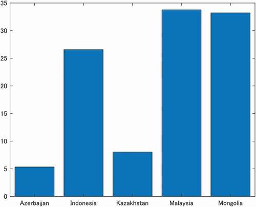
It is beyond the scope of this study to explain the lack of a relationship between their exporting commodity prices and interest spreads in Azerbaijan and Kazakhstan. However, a possible explanation can be found in the fact that levels of financial inclusion in Azerbaijan and Kazakhstan are further below those in the other three countries (Figure 2). In other words, financial institutions and markets in Azerbaijan and Kazakhstan may be too underdeveloped to be deeply integrated into the world financial market and receive some influence from the world financial market’s fluctuations. If this is the case, it would be plausible that, since Azerbaijan and Kazakhstan are not under financial friction, fluctuations in their exporting commodity prices do not affect their interest spreads.

Figure 2. Percentage having saved at a financial institution in the past year, 2014 (% age 15+, Series Code: fin17a.t.a). Source: World Bank Global Financial Inclusion Database

IV. Conclusion

This note shows that world commodity price shocks have a significant impact on Asian commodity exporting economies. The result of the SVAR impulse responses suggests that the recent drop in world commodity prices due to the COVID-19 shock may have a significant negative impact on output, consumption, and investment in these economies. As for the trade balance, we find that the sample countries are divided into two groups: Malaysia, Mongolia, and Indonesia may have positive trade balances, while Azerbaijan and Kazakhstan may have negative trade balances. The differences between these two groups found in the SVAR analysis results can likely be attributed to the effect of world commodity prices on the interest rate spreads of each country. In Malaysia, Mongolia, and Indonesia, a fall in world commodity prices has a negative effect on their interest rate spreads, which leads to a decline in their foreign borrowing, i.e. a trade balance surplus. However, in Azerbaijan and Kazakhstan, the effect of world commodity price fluctuations is neutral on their interest rate spreads. In these countries, therefore, the effect of a fall in world commodity prices is straightforward, as shown in a standard textbook on open economy macroeconomics. Since a temporary fall in exporting commodity prices corresponds to a temporary negative income shock, these economies would finance the negative income shock by borrowing from the rest of the world through a deterioration in their trade balances.

There are some limitations to this study. First, although, following ADB (2016), we treat Azerbaijan, Indonesia, Kazakhstan, Malaysia, and Mongolia as sample countries in this study due to data limitations, it would be more desirable to include additional countries. Second, as we argue in Section 2, the large fluctuation in Mongolia’s investment and positive response in Indonesia’s consumption are not given a clear explanation. Finally, as we argue in Section 3, although we provide a possible explanation related to their financial inclusion levels, further analysis may be needed to give a more rigorous reason for the lack of a relationship between exporting commodity prices and interest spreads in Azerbaijan and Kazakhstan. We leave these points for future work.

Acknowledgments

I am grateful to an anonymous referee for the encouraging comments. I am also grateful to Shugo Yamamoto, Toshiki Jinushi, Masahiko Shibamoto, and Kenya Takaku for their helpful comments.

Disclosure statement

No potential conflict of interest was reported by the author.

Additional information

Funding

This work is supported by JSPS KAKENHI [16K03741, 20K01744].

Notes

¹ For example, Shousha (2016) considers Argentina, Brazil, Chile, Colombia, Peru and South Africa as emerging economies and Australia, Canada, New Zealand and Norway as advanced economies. Drechsel and Tenreyro (2018) use data on Argentina. The sample counties included in Bastourre et al. (2012) are Argentina, Brazil, Bulgaria, Colombia, Ecuador, Malaysia, Mexico, Panama, Peru, Poland, Russia, Turkey, and Venezuela. Fernández, González, and Rodriguez (2018) uses data on Brazil, Chile, Colombia, and Peru for SVAR analysis.

² Specifically, we choose the five countries included in Table 3 on page 19 in ADB (2016).

³ The raw data are available at http://www.worldbank.org/commodities. Taking averages across the months in a given quarter, we convert monthly commodity indices into quarterly indices.

⁴ The source for the US CPI is the Federal Reserve Bank of St. Louis FRED Database: https://fred.stlouisfed.org.

⁵ Although, following World Bank (2016), we use the US CPI in the multi-country analysis due to data availability constraints, the use of import prices or any other cost-related prices might be interesting to consider wealth and substitution effects in a specific country analysis.

⁶ The WITS data base is available at https://wits.worldbank.org/.

⁷ See, for example, Sims, Stock, and Watson (1990), Hamilton (1994, 652), and Kilian and Lütkepohl (2017, 373–7).

⁸ As for GDP deflator, quarterly data is not available for Azerbaijan, Kazakhstan, and Mongolia. For these countries, we convert annual data to quarterly data.

⁹ The SVAR model contains two lags, and is chosen taking into account several lag length selection criteria. Specifically, we take AIC, SC, and HQ criteria into consideration. Since in the case of Azerbaijan the three criteria show that appropriate lag length is one, we checked how the impulse response with one lag differs from that with two lags, and confirmed that our main implications do not change.

¹⁰ The raw quarterly series are seasonally adjusted. As for the GDP deflator, quarterly data are not available for Azerbaijan, Kazakhstan, and Mongolia. For these countries, we convert annual data to quarterly data.

¹¹ The raw quarterly series are seasonally adjusted.

¹² Output, exports, and imports are obtained from IFS. The raw series are seasonally adjusted and transformed to real terms using the GDP deflator.

¹³ The raw annual series are obtained from IMF Global Debt Database. We convert the raw annual data to quarterly data.

¹⁴ Among many, for example, see Végh (2013) and Schmitt-Grohé and Uribe (2017).

¹⁵ ”Output” is omitted due to low performance.

¹⁶ The data source is IMF Global Debt Database. We convert the raw annual data to quarterly data.

AppendixA1

Additional regression result in Section 3

In Section 3, following the related studies (Drechsel and Tenreyro 2018; Bastourre et al. 2012; Fernández, González, and Rodriguez 2018), we considered government debt in our empirical analysis. In this appendix, we incorporate private debt in addition to the government debt in our regression.¹⁵

In Table A1, ‘Private debt’ is total private debt (loans and debt securities) as a share of GDP.¹⁶ The first row of the table shows that the coefficients on international commodity prices, $\xi$, remain significant and negative for Malaysia, Mongolia, and Indonesia as in the main text. On the other hand, the coefficients on international commodity prices, $\xi$, remain not significant for Azerbaijan and Kazakhstan as in the main text. Therefore, we can confirm that our main results do not change even when we include private debt in addition to the government debt.

Table A1. Regression results in the case with government and private debt

	Interest rate spreads
LHS variable	MAL	MON	IND	AZE	KAZ
Commodity price	−0.042***	−0.286***	−0.256***	0.086	0.008
	(0.011)	(0.053)	(0.049)	(0.061)	(0.021)
Trade balance	−0.042	−0.310***	−1.728***	−0.031	−0.098
	(0.032)	(0.078)	(0.315)	(0.076)	(0.093)
Government debt	0.192***	−0.121	0.242***	0.364	0.414***
	(0.039)	(0.114)	(0.054)	(0.258)	(0.080)
Private debt	0.020	−0.009	−0.360***	0.124	−0.006
	(0.018)	(0.081)	(0.055)	(0.096)	(0.033)
Constant	−0.100***	0.158***	0.124***	0.035	−0.075***
	(0.027)	(0.040)	(0.025)	(0.030)	(0.022)

Standard errors in parentheses. *** p < 0.01, ** p < 0.05, and * p < 0.1.

Note: ‘Trade balance’, ‘Government debt’, and ‘Private debt’ denote their ratios to GDP. The sample periods are as follows: Malaysia, 1992Q1–2018Q4; Mongolia, 2005Q1–2018Q1; Indonesia, 1998Q1–2018Q3; Azerbaijan, 2001Q1–2016Q4; Kazakhstan, 2000Q1–2017Q3.

References

- ADB. 2016. “Moderating Growth and Structural Change in the People’s Republic of China: Implications for Developing Asia and Beyond.” ADB Reports ABF167930-2, Asian Development Bank.
- Bastourre, D., J. Carrera, J. Ibarlucia, and M. Sardi. 2012. “Common Drivers in Emerging Market Spreads and Commodity Prices.” BCRA Working Paper Series 201257, Central Bank of Argentina, Economic Research Department.
- Drechsel, T., and S. Tenreyro. 2018. “Commodity Booms and Busts in Emerging Economies.” Journal of International Economics 112: 200–218. doi:https://doi.org/10.1016/j.jinteco.2017.12.009.
- Fernández, A., A. González, and D. Rodriguez. 2018. “Sharing a Ride on the Commodities Roller Coaster: Common Factors in Business Cycles of Emerging Economies.” Journal of International Economics 111: 99–121. doi:https://doi.org/10.1016/j.jinteco.2017.11.008.
- Hamilton, J. D. 1994. Time Series Analysis. Princeton, N.J.: Princeton University Press.
- Hevia, C., and A. Neumeyer. 2020. “A Conceptual Framework for Analyzing the Economic Impact of Covid-19 and Its Policy Implications.” UNDP LAC C19 PDS No.1, UNDP Latin American and the Cribbean.
- Kilian, L., and H. Lütkepohl. 2017. Structural Vector Autoregressive Analysis, Themes in Modern Econometrics. Cambridge: Cambridge University Press.
- Schmitt-Grohé, S., and M. Uribe. 2017. Open Economy Macroeconomics. Princeton, N.J.: Princeton University Press.
- Shousha, S. 2016. “Macroeconomic Effects of Commodity Booms and Busts: The Role of Financial Frictions.” unpublished manuscript.
- Sims, C. A., J. H. Stock, and M. W. Watson. 1990. “Inference in Linear Time Series Models with Some Unit Roots.” Econometrica 58 (1): 113–144. doi:https://doi.org/10.2307/2938337.
- Sims, C. A., and T. Zha. 1999. “Error Bands for Impulse Responses.” Econometrica 67 (5): 1113–1155. doi:https://doi.org/10.1111/1468-0262.00071.
- Végh, C. A. 2013. Open Economy Macroeconomics in Developing Countries. Cambridge:MIT Press.
- World Bank. 2016. Global Economic Prospects, January 2016: Spillovers amid Weak Growth. Washington, DC: World Bank.