A dynamic leverage stochastic volatility model

ABSTRACT

Stock returns are considered as a convolution of two random processes that are the return innovation and volatility innovation. The correlation of these two processes tends to be negative, which is the so-called leverage effect. In this study, we propose a dynamic leverage stochastic volatility (DLSV) model where the correlation structure between the return innovation and the volatility innovation is assumed to follow a generalized autoregressive score (GAS) process. We find that the leverage effect is reinforced in the market downturn period and weakened in the market upturn period.

KEYWORDS:

• Dynamic leverage
• GAS
• stochastic volatility (SV)

JEL CLASSIFICATION:

• C59
• C11

I. Introduction

Stock returns are considered as a convolution of two random processes that are the volatility and return innovation. The correlation of these two processes tends to be negative, which is the so-called leverage effect. One explanation for this leverage effect is that the negative shock to the return may increase the financial leverage ratio between debt and equity. Therefore, the stock becomes riskier, which results in higher volatility. The leverage response between volatility and return news was initially analyzed by Black (1976) and further supported by the research of Nelson (1991), and Harvey and Shephard (1996), among others. However, a majority of studies consider constant leverage over time which is a rather restrictive assumption. On the other hand, time-varying leverage has been documented in several studies, see Bandi and Renò (2012), Yu (2012), Bretó (2014), among others. The dynamic leverage not only helps to derive a better prediction of the volatility process but also can influence asymmetrically on the volatility smiles (Veraart and Veraart 2012).

In this study, we focus on the driven factors of the leverage effect by proposing a dynamic leverage stochastic volatility (DLSV) model where the correlation structure between the return innovation and volatility innovation is assumed to follow a generalized autoregressive score (GAS) process, see Creal, Koopman, and Lucas (2013). As the correlation is driven by an observation-driven process, the number of latent parameters that need to be estimated is significantly smaller than that of a parameter-driven process, hence the estimation is computationally less expensive. It is also straightforward to extend the current proposed inference algorithm for the fixed leverage stochastic volatility (LSV) model to a dynamic setting with a small marginal cost of computation. We take a Bayesian approach for statistical inference in DLSV and employ the annealing sequential Monte Carlo (ASMC) algorithm of Tran et al. (2014) and Duan and Fulop (2015) for posterior approximation. ASMC is an efficient sampler for Bayesian inference that combines the anneal important sampling of Neal (2001) and the sequential Monte Carlo method of Del Moral, Doucet, and Jasra (2006).

We find that the sign and magnitude of the temporal return innovations are the main factors that encourage the leverage effect. The leverage effect is strengthened in the market downturn period and is weakened in the market upturn period. The DLSV model improves the in-sample fit in comparison to the fixed leverage stochastic volatility (LSV) model.

II. Model

Let $\{y_t,t=1,\dots ,T\}$ be the time series of financial returns. Harvey and Shephard (1996) proposed the LSV model based on the SV model of Taylor (1986). The model assumes a fixed intertemporal correlation between the lag return innovation and volatility innovation despite price movement as follows:

(1) $\begin{array}{cc}{y}_t& =exp(0.5h_t){ϵ}_t,\\ h_t& ={\mu }_h(1-\varphi )+\varphi h_{t-1}+{\sigma }_{\eta }{\eta }_t,\\ {\eta }_t& =\rho {\epsilon }_{t-1}+\sqrt{1-{\rho }^2}{\zeta }_t,\end{array}$(1)

where $h_t$ is the log volatility of the financial return, ${\epsilon }_t$ is the return innovation and ${\eta }_t$ is the volatility innovation which correlates with ${\epsilon }_{t-1}$. The innovations ${\epsilon }_t$ and ${\zeta }_t$ are assumed to be mutually independent variables that follow standard Normal distributions. The latent volatility process $h_t$ is specified by the mean parameter ${\mu }_h$, the persistence parameter $|\varphi |<1$ and the volatility parameter ${\sigma }_{\eta }>0$. The leverage effect between shocks and volatility is captured through the dependence between ${\epsilon }_{t-1}$ and ${\eta }_t$ in the sense that given $\rho <0$, a negative shock to the returns is likely to result in an increase in the volatility. Differently, Jacquier, Polson, and Rossi (2004) proposed an alternative specification for the contemporaneous relation. Yu (2005) compared these two models and concluded that the model of Harvey and Shephard (1996) is an Euler approximation of the continuous time SV model, which is also supported by empirical analysis. Recently, Catania (2020) introduced a generalization of these two models by adding more temporal return innovation lags in the volatility innovation equation. However, there is evidence that the relation between the return innovation and volatility innovation is dynamic. Yu (2012) generalized the correlation structure in the LSV model using a linear spline and found a strong evidence against the fixed leverage effect. Bretó (2014) analyzed the S&P 500 return using an idiosyncratic stochastic leverage model and confirmed the random walk LSV model outperforms the fixed LSV model.

On the other hand, we extend Equation 1(1) $\begin{array}{cc}{y}_t& =exp(0.5h_t){ϵ}_t,\\ h_t& ={\mu }_h(1-\varphi )+\varphi h_{t-1}+{\sigma }_{\eta }{\eta }_t,\\ {\eta }_t& =\rho {\epsilon }_{t-1}+\sqrt{1-{\rho }^2}{\zeta }_t,\end{array}$(1) and allow for the dynamic leverage effect by allowing ${\rho }_t$ to follow a GAS process as follows

(2) $\begin{array}{rl}& {\eta }_t={\rho }_t{\epsilon }_{t-1}+\sqrt{1-{\rho }_t^2}{\zeta }_t,\\ & {\rho }_t=\frac{exp(f_t)-1}{exp(f_t)+1},\\ & f_t=\omega (1-b)+a{s}_{t-1}+b{f}_{t-1},\\ & s_{t-1}=\frac{\mathrm{\partial }logp(y_{t-1}|f_{t-1})}{\mathrm{\partial }{f}_{t-1}}=\frac{\mathrm{\partial }logp(y_{t-1}|f_{t-1})}{\mathrm{\partial }{h}_{t-1}}\frac{\mathrm{\partial }{h}_{t-1}}{\mathrm{\partial }{\rho }_{t-1}}\frac{\mathrm{\partial }{\rho }_{t-1}}{\mathrm{\partial }{f}_{t-1}}\\ & =\frac{1}{2}({\epsilon }_{t-1}^2-1){\sigma }_{\eta }\left({\epsilon }_{t-2}-\frac{{\rho }_{t-1}}{\sqrt{1-{\rho }_{t-1}^2}}{\zeta }_{t-1}\right)\frac{2exp(f_{t-1})}{{(exp(f_{t-1})+1)}^2}.\end{array}$(2)

So that $Corr({\eta }_t,{\epsilon }_{t-1})={\rho }_t$. We ensure the value of ${\rho }_t\in [-1,1]$ by using a transformation function of a GAS process $f_t$. The process $f_t$ is an observation-driven process that is specified by the mean parameter $\omega$, the persistence parameter $b$ and an adjustment term calculated as a score function $s_{t-1}$. Here, we restrict $0\le b<1$ for the stationary condition, see Creal, Koopman, and Lucas (2013). The updated score depends on both the sign and magnitude of the return innovations which leads to the change in the leverage effect. In this case, there is only one score value for each time period as only the volatility of the returns is time-varying. We take advantage of this score to explain the dynamic leverage effect rather than the volatility dynamic like what has been done in the leverage Beta-$t$-EGARCH model (Harvey and Chakravarty 2008), because if the score is used to explain both the volatility and leverage effect, there is no incentive to use the score again to construct the dynamic leverage in the Beta-$t$-EGARCH model. In the DLSV model, the score function provides a signal for updating the volatility process $h_t$ in the sense that the prediction of the volatility process would be more accurate when the magnitude $|{\rho }_t|$ is higher. Blasques, Koopman, and Lucas (2015) show that the use of the score functions is robust to the model misspecification and leads to the minimization of the Kullback–Leibler divergence between the true conditional density and the model-implied conditional density. We note that when $a=b=0$, the model becomes a fixed LSV model. Also, when $a=b=\omega =0$, we obtain the SV model without leverage effect.

We employ the ASMC algorithm of Tran et al. (2014) and Duan and Fulop (2015) to make Bayesian inference on the parameters of interest. In general, the ASMC samples sequentially from the prior distribution to the target posterior distribution through a sequence distribution that smoothly interpolates between the prior and the posterior distribution. The ASMC also provides the marginal likelihood estimate, which is useful for model comparison. Let us denote $\theta =({\mu }_h,\varphi ,{\sigma }_{\eta },\omega ,a,b)$ the set of fixed parameters in the DLSV model. We use vague but proper prior distributions for the parameters of the DLSV model. The priors are more informative in comparison to Kastner and Frühwirth-Schnatter (2014) to prevent the bad particles at the early stage of tempering. For the parameters in the volatility process, their priors are ${\mu }_h\sim \mathcal{N}(0,1)$, $\varphi \sim \mathrm{B}\mathrm{e}\mathrm{t}\mathrm{a}(20,1.5)$ and ${\sigma }_{\eta }^2\sim \mathrm{G}\mathrm{a}\mathrm{m}\mathrm{m}\mathrm{a}(\frac{1}{2},\frac{1}{2B_{\sigma }})$, which is equivalent to $\pm \sqrt{{\sigma }_{\eta }^2}\sim \mathcal{N}(0,B_{\sigma })$. For the parameters in the GAS process, we consider the following priors: $\omega \sim \mathcal{N}(0,2)$, $a\sim \mathcal{N}(0,1){\mathbf{I}}_{\{a>0\}}$, $b\sim \mathrm{B}\mathrm{e}\mathrm{t}\mathrm{a}(30,1)$. For the fixed LSV model, we assume that the fixed parameter $\rho \sim \mathbf{U}(-1,1)$.

III. Empirical illustration

This section illustrates the performance of the proposed DLSV model using three daily stock return indexes: the Dow Jones Industrial Average index (DJI), the Financial Times Stock Exchange 100 index (FTSE) and the Nikkei 225 stock index (NIKKEI). The data is obtained from the Macrobond database during the period from 1 January 1990 to 31 December 2017. The returns are calculated as the first difference of the log of the stock index multiplied by 100. Table 1 describes their summary statistics. All the return series show some degree of heavier tails than the normal distribution and serial correlations.

Table 1. Summary statistics of the three stock returns (1 January 1990 – 31 December 2017)

	Mean	Std.	Skewness	Kurtosis	Minimum	Maximum	J-B test	Ljung-Box(12)	ARCH(12)
DJI	0.031	1.057	−0.170	8.394	−8.200	10.508	20.729***	65.453***	1741.386***
FTSE	0.016	1.101	−0.127	6.067	−9.266	9.384	10.874***	78.307***	1581.783***
NIKKEI	−0.008	1.522	−0.130	5.397	−12.111	13.235	8.381***	24.844***	1202.434***

***,**,* denote significant at 1%, 5%, 10% levels, respectively.

The table reports the summary statistics of the three stock indexes. We report the test statistics of the Jarque-Bera test for normality, the Ljung-Box test for the serial correlation and ARCH test for the GARCH effect.

Next, we demean each of the return series and estimate the model parameters of the SV model without leverage, the LSV model and the proposed DLSV model using the ASMC sampler. Table 2 reports the posterior mean estimates of the parameters. The credible interval of parameters $a$ and $b$ is significantly different from 0, which shows that the leverage effect is time-varying. The averages of the leverage effect are very similar between the LSV model and the DLSV model. However, the DLSV improves the marginal likelihood over the SV and the LSV models.

Table 2. Posterior estimates for the in-sample data (1 January 1990 – 31 December 2017)

Model	${\mu }_h$	$\varphi$	${\sigma }_{\eta }$	$\rho$	$a$	$b$	LLH
(a) DJI
SV	−0.387	0.976	0.044				−8973.318
	(−0.514;-0.258)	(0.972;0.981)	(0.037;0.051)
LSV	−0.364	0.975	0.042	−0.650			−8852.364
	(−0.462;-0.265)	(0.971;0.979)	(0.036;0.049)	(−0.688;-0.609)
DLSV	−0.371	0.977	0.039	−0.639	0.486	0.983	−8844.172
	(−0.456;-0.286)	(0.973;0.981)	(0.033;0.045)	(−0.695;-0.547)	(0.172;0.787)	(0.946;0.999)
(b) FTSE
SV	−0.231	0.980	0.029				−9468.208
	(−0.356;-0.106)	(0.976;0.984)	(0.025;0.034)
LSV	−0.237	0.983	0.025	−0.685			−9359.464
	(−0.352;-0.123)	(0.980;0.986)	(0.021;0.029)	(−0.726;-0.640)
DLSV	−0.246	0.985	0.024	−0.702	0.700	0.990	−9347.305
	(−0.354;-0.139)	(0.983;0.988)	(0.020;0.028)	(−0.750;-0.646)	(0.259;1.203)	(0.980;0.999)
(c) NIKKEI
SV	0.469	0.966	0.044				−11792.990
	(0.372;0.565)	(0.961;0.972)	(0.038;0.051)
LSV	0.467	0.964	0.047	−0.563			−11692.408
	(0.392;0.543)	(0.958;0.969)	(0.040;0.054)	(−0.607;-0.519)
DLSV	0.482	0.965	0.045	−0.565	0.516	0.973	−11686.520
	(0.395;0.565)	(0.959;0.969)	(0.039;0.052)	(−0.612;-0.510)	(0.141;0.950)	(0.932;0.997)

The table reports the posterior means of the parameters of SV, LSV and DLSV models, together with the marginal likelihood estimates in the last column. The average leverage effect in the DLSV model is computed as $\rho =\frac{exp(\omega )-1}{exp(\omega )+1}$ for the ease of comparison. The ASMC sampler is run with $M=1000$ particles. The numbers in the bracket show the [10% – 90%] credible intervals.

Figure 1 shows the filtered volatility and the filtered dynamic leverage effect. The patterns of the filtered volatility are similar among all series. Even though the leverage effect of the NIKKEI series is weakest, and it is more volatile at the end of the sample. On the other hand, the dynamic leverage effect of the DJI is quite stable through time, while that of the FTSE is decreasing. We do not observe a strong relationship between the change in the dynamic leverage effect and the level of the volatility, which is similar to the findings of Yu (2012) and Bretó (2014).

Figure 1. The filtered volatility and the filtered dynamic leverage effect

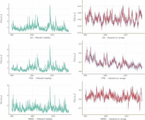
The left-hand side figure plots the filtered volatility, and the right-hand side figure plots the filtered dynamic leverage effect in red colour with their 50% credible interval in blue colour. The results were obtained using a particle filter with 10,000 particles.

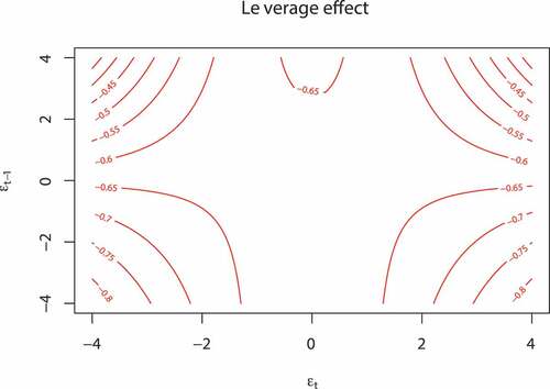
We analyze the effect of the temporal return innovations (${\epsilon }_t,{\epsilon }_{t-1}$) on the correlation ${\rho }_{t+1}$. Using Equation 2(2) $\begin{array}{rl}& {\eta }_t={\rho }_t{\epsilon }_{t-1}+\sqrt{1-{\rho }_t^2}{\zeta }_t,\\ & {\rho }_t=\frac{exp(f_t)-1}{exp(f_t)+1},\\ & f_t=\omega (1-b)+a{s}_{t-1}+b{f}_{t-1},\\ & s_{t-1}=\frac{\mathrm{\partial }logp(y_{t-1}|f_{t-1})}{\mathrm{\partial }{f}_{t-1}}=\frac{\mathrm{\partial }logp(y_{t-1}|f_{t-1})}{\mathrm{\partial }{h}_{t-1}}\frac{\mathrm{\partial }{h}_{t-1}}{\mathrm{\partial }{\rho }_{t-1}}\frac{\mathrm{\partial }{\rho }_{t-1}}{\mathrm{\partial }{f}_{t-1}}\\ & =\frac{1}{2}({\epsilon }_{t-1}^2-1){\sigma }_{\eta }\left({\epsilon }_{t-2}-\frac{{\rho }_{t-1}}{\sqrt{1-{\rho }_{t-1}^2}}{\zeta }_{t-1}\right)\frac{2exp(f_{t-1})}{{(exp(f_{t-1})+1)}^2}.\end{array}$(2) , we show the contour plot of the correlation ${\rho }_{t+1}$ on the DJI temporal return innovations in Figure 2. Here, the GAS process $f_t$ is assumed to stay at its long-term mean $\omega$ and ${\zeta }_t=0$. According to the sign and magnitude of (${\epsilon }_t,{\epsilon }_{t-1}$), the leverage effect is reinforced when observing both strong temporal negative return shocks which is in contrast to when observing both strong temporal positive return shocks. The leverage is weakened during the uncertain market gain (${\epsilon }_{t-1}>0,{\epsilon }_t<0$), and it is strengthened during the uncertain market loss (${\epsilon }_{t-1}<0,{\epsilon }_t>0$).

Figure 2. The contour plot shows the impact of the temporal return innovations (${\epsilon }_t,{\epsilon }_{t-1}$) on the dynamic leverage correlation ${\rho }_{t+1}$ for the DJI data. The current GAS process $f_t$ is assumed to stay at its long-term mean $\omega$ and ${\zeta }_t=0$

IV. Conclusion

In this study, we propose a dynamic LSV model where the correlation structure between the return innovation and volatility innovation is assumed to follow a GAS process. We find that the DLSV model improves the in-sample fit in comparison to the fixed leverage effect LSV model and the standard SV model. Our key finding is that the leverage effect is reinforced in the market downturn period and is weakened in the market upturn period.

Acknowledgments

The computations were enabled by resources provided by the Swedish National Infrastructure for Computing (SNIC) at HPC2N, partially funded by the Swedish Research Council through grant agreement no. 2018-05973. Financial support from Jan Wallanders and Tom Hedelius Foundation (grants number BV18-0018) is gratefully acknowledged.

Disclosure statement

No potential conflict of interest was reported by the author(s).

Correction Statement

This article has been republished with minor changes. These changes do not impact the academic content of the article.

Additional information

Funding

This work was supported by the Jan Wallanders och Tom Hedelius Stiftelse samt Tore Browaldhs Stiftelse [BV18-0018]; Swedish National Infrastructure for Computing [2018-05973].

References

- Bandi, F. M., and R. Renò. 2012. “Time-varying Leverage Effects.” Journal of Econometrics 169 (1): 94–113. doi:10.1016/j.jeconom.2012.01.010.
- Black, F. 1976. “Studies of Stock Market Volatility Changes.” In Proceedings of the American Statistical Association, Business and Economics Statistics Section, 177–181.
- Blasques, F., S. Koopman, and A. Lucas. 2015. “Information-theoretic Optimality of Observation-driven Time Series Models for Continuous Responses.” Biometrika 102 (2): 325–343. doi:10.1093/biomet/asu076.
- Bretó, C. 2014. “On Idiosyncratic Stochasticity of Financial Leverage Effects.” Statistics & Probability Letters 91: 20–26. doi:10.1016/j.spl.2014.04.003.
- Catania, L. 2020. “A Stochastic Volatility Model with A General Leverage Specification.” Journal of Business & Economic Statistics 1–23. doi:10.1080/07350015.2020.1840994.
- Creal, D., S. J. Koopman, and A. Lucas. 2013. “Generalized Autoregressive Score Models with Applications.” Journal of Applied Econometrics 28 (5): 777–795. doi:10.1002/jae.1279.
- Del Moral, P., A. Doucet, and A. Jasra. 2006. “Sequential Monte Carlo Samplers.” Journal of the Royal Statistical Society: Series B (Statistical Methodology) 68 (3): 411–436. doi:10.1111/j.1467-9868.2006.00553.x.
- Duan, J.-C., and A. Fulop. 2015. “Density-tempered Marginalized Sequential Monte Carlo Samplers.” Journal of Business & Economic Statistics 33 (2): 192–202. doi:10.1080/07350015.2014.940081.
- Harvey, A. C., and T. Chakravarty. 2008. “Beta-t-(e)garch.” CWPE 08340, Faculty of Economics, University of Cambridge.
- Harvey, A. C., and N. Shephard. 1996. “Estimation of an Asymmetric Stochastic Volatility Model for Asset Returns.” Journal of Business & Economic Statistics 14 (4): 429–434.
- Jacquier, E., N. G. Polson, and P. E. Rossi. 2004. “Bayesian Analysis of Stochastic Volatility Models with Fat-tails and Correlated Errors.” Journal of Econometrics 122 (1): 185–212. doi:10.1016/j.jeconom.2003.09.001.
- Kastner, G., and S. Frühwirth-Schnatter. 2014. “Ancillarity-sufficiency Interweaving Strategy (ASIS) for Boosting MCMC Estimation of Stochastic Volatility Models.” Computational Statistics & Data Analysis 76: 408–423. doi:10.1016/j.csda.2013.01.002.
- Neal, R. M. 2001. “Annealed Importance Sampling.” Statistics and Computing 11 (2): 125–139. doi:10.1023/A:1008923215028.
- Nelson, D. B. 1991. “Conditional Heteroskedasticity in Asset Returns: A New Approach.” Econometrica 59 (2): 347–370. doi:10.2307/2938260.
- Taylor, S. J. 1986. Modelling Financial Time Series. Chichester, UK: John Wiley.
- Tran, M.-N., M. Scharth, M. K. Pitt, and R. Kohn. 2014. “Annealed Important Sampling for Models with Latent Variables.” arXiv preprint arXiv:1402.6035.
- Veraart, A. E., and L. A. Veraart. 2012. “Stochastic Volatility and Stochastic Leverage.” Annals of Finance 8 (2–3): 205–233. doi:10.1007/s10436-010-0157-3.
- Yu, J. 2005. “On Leverage in a Stochastic Volatility Model.” Journal of Econometrics 127 (2): 165–178. doi:10.1016/j.jeconom.2004.08.002.
- Yu, J. 2012. “A Semiparametric Stochastic Volatility Model.” Journal of Econometrics 167 (2): 473–482. doi:10.1016/j.jeconom.2011.09.029.