Forecasting cryptocurrencies’ price with the financial stress index: a graph neural network prediction strategy

ABSTRACT

This article proposes a graph neural network strategy (GNN), in which the long short-term memory (LSTM) and graph convolution network (GCN) are applied to capture both temporal and spatial features to forecast the price of Bitcoin, Litecoin, Ethereum, and Dash Coin with the ‘stable-coin’ Tether (USDT) and financial stress index (FSI). The main results show that the GNN strategy has better performance than univariate LSTM and multivariate LSTM in all of the seven steps forward forecasting. A sensitivity check shows that USDT and FSI/sub-FSI are important factors in the construction of the graphs and they verify the validity of the results.

KEYWORDS:

• Graph neural network
• cryptocurrency price
• time-series forecast
• financial stress index

JEL CLASSIFICATION:

• C53
• G15
• G17

I. Introduction

Cryptocurrencies have graduated from being a niche investment to a major global investment asset. This development has seen an increasing interaction with the global ‘traditional’ financial market. The key factor that links the financial market to the cryptocurrency market is the flow of liquidity, which is driven by the activity of investors, traders, hedgers, and speculators as they move in and out of cryptocurrencies. Recently, major economies have issued strict regulations on cryptocurrency trading in an attempt to obstruct the shocks from cryptocurrencies impacting the financial system. The Tether (USDT) peg to the value of USD, which is called a ‘stable-coin’, serves as a bridge to facilitate the flow of money between the two sides. An increasingly complex connection has been observed between financial market and crypto-asset market through price volatility (Giudici and Abu-Hashish 2019; Giudici and Polinesi 2021). Therefore, network structure analysis is increasingly being used by researchers. Based on previous studies, this article proposes a graph network prediction strategy to forecast the price of Bitcoin, Litecoin, Ethereum, and Dash Coin simultaneously, while combining time-series and network dimensions.

Bitcoin returns have a complex relationship with the investors’ risk revision level (Bouri et al. 2021). The connectedness of Bitcoin exchange platforms varies over time. For instance, a leading exchange such as Bitfinex has a spillover effect on other exchanges (Giudici and Pagnottoni 2019, 2020). Similar to financial markets, the prediction model is based on intraday momentum and reversal can be applied in cryptocurrencies trading market (Wen et al. 2022). On the macro-level, Bitcoin has been found to be a safe haven against global financial stress based on quantile dependence analysis (Bouri et al. 2018). Moreover, Wang, Sarker, and Bouri (2022) employ several wavelet-related methods with US data and find that the impact of Bitcoin price on money supply is significant.

Beyond dealing with time-series data itself, research has recently moved towards graph prediction. Kim and Kim (2019) propose a fusion LSTM convolutional neural network (LSTM-CNN) model, which simultaneously captures the temporal and image features of stock data. The results show that the prediction method with image performance is better than only using the same time-series data. To solve the problems of noisy signals and missing data, Lewenfus et al. (2020) propose a combination of graph signal process with deep learning in multivariate time-series prediction. Liu et al. (2021) convert stock price into chart images and then use deep learning neural networks (DLNNs) to perform the forecasting. Their model obtains an average accuracy rate of 55.46% when applying Chinese stock data from 2009 to 2020. Cheng et al. (2022) designed a multi-dimensional GNN prediction framework together with several algorithms. Their test results show that the GNN performs well when applying financial time series. In addition to forecasting price changes, Wei, Zhang, and Liu (2021) set graphs to capture different types of spatial-temporal Bitcoin transaction patterns and forecast the transaction behaviour.

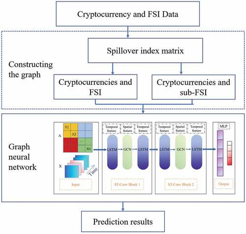
Based on these previous studies, this article contributes to the limited existing literature on cryptocurrency price predation in four ways. First, this article forecasts the price of four main cryptocurrencies instead of only focusing on Bitcoin to capture the intrinsic interactions among cryptocurrencies. Second, this article includes the financial stress index (FSI) in the graph to make the prediction, which is able to capture the bilateral spillover effect between the cryptocurrency market and the traditional financial market. Third, considering the important role of USDT for money flowing in the financial system, this article embeds USDT as a node into the graph. Finally, the method developed by Diebold and Yilmaz (2009) is applied in this article to obtain the spillover index of the variables as the values of the boundaries between each node in the graph, which enables the application of the GNN strategy. The overall research framework is given in Figure 1.

Figure 1. Framework of the model.

Note: the formulations of mathematical terms for GNN are given in the appendix.

II. Main results

The details of data and methodology are given in the appendix. We use max-min normalization to deal with the original data to eliminate dimensional differences. The sample data were linearly transformed into the range of [0, 1]. We then obtain the final results and transfer the prediction data back through the reverse process of the normalization. To test the GNN’s prediction performance, following the relevant previous studies (e.g. Kim and Kim 2019; Lewenfus et al. 2020), this article employs univariate and multivariate LSTM for comparison. The parameter settings of the deep learning methods are given in Table 1.

Table 1. Parameter settings of the deep learning methods.

	GNN	Univariate LSTM	Multivariate LSTM
Activation	relu	tanh	tanh
Dropout	0	0	0
History step	10	1	10
Batch_size	50	1	16
Epochs	50	50	50
LR	0.001	0.001	0.001
Optimizer	RMSprop	adam	adam

Similar to previous studies, Mean Absolute Error (MAE), Mean Absolute Percentage Error (MAPE), and Root Mean Square Error (RMSE) are selected here as a performance assessment. The results of different prediction steps (from +1 day to +7 days) are given in Table 2.

Table 2. Comparing prediction errors of GNN using FSI with other models.

		GNN using FSI	GNN using sub-FSI	Univariate LSTM	Multivariate LSTM
+1 day	MAE	0.275	0.230	1.235	4.924
	MAPE	0.065	0.124	0.085	0.090
	RMSE	0.676	0.675	1.510	4.590
+2 days	MAE	0.378	0.296	1.786	3.881
	MAPE	0.096	0.186	0.090	0.073
	RMSE	0.817	0.783	1.990	4.820
+3 days	MAE	0.404	0.320	1.854	4.015
	MAPE	0.105	0.175	0.092	0.075
	RMSE	0.906	0.821	2.169	5.564
+4 days	MAE	1.409	0.862	1.644	5.430
	MAPE	0.155	0.297	0.095	0.099
	RMSE	3.236	2.306	2.282	6.255
+5 days	MAE	1.218	2.168	1.692	4.883
	MAPE	0.153	0.314	0.101	0.090
	RMSE	2.717	5.845	2.053	5.661
+6 days	MAE	0.601	1.046	1.731	5.129
	MAPE	0.104	0.214	0.098	0.095
	RMSE	1.506	2.949	1.904	5.710
+7 days	MAE	2.119	1.952	1.818	5.275
	MAPE	0.275	0.260	0.096	0.098
	RMSE	4.887	5.137	2.342	6.732

Note: The definitions of MAE, MAPE, and RMSE are given in Table A4 in the appendix.

It can be observed that the GNN strategy gives a better prediction result than univariate and multivariate LSTM in each of the prediction steps. Specifically, the performance of GNN with FSI strategy is better in prediction step +4 days, +5 days, and +6 days, while GNN with sub-FSI strategy gives a better result in prediction +7 days. These results suggest that FSI has a significant relationship with cryptocurrencies, which is similar to the findings of Bouri et al. (2018) showing bilateral effects between the global financial stress index and Bitcoin returns. However, it is difficult to clearly distinguish the performance between the two GNN methods in the prediction step of +1 day, +2 days, and +3 days. GNN with FSI method has lower MAPE but higher MAE and RMSE when comparing GNN with sub-FSI in the first four prediction steps.

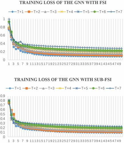
In general, MAE, MAPE and RMSE become larger as the prediction steps increase from +1 day to +4 days, which shows that the accuracy and robustness of the long prediction is weaker than the short prediction. This result is consistent with the expectations of similar research. As shown in Figure 2, the training loss of the GNN with FSI decreases quickly and becomes convergent after seven epochs. Meanwhile, the training loss of the GNN with sub-FSI has the same trend and becomes convergent after four epochs. Moreover, the training loss is more clustered in the GNN with sub-FSI, which shows that this method has better fitting in general.¹ This article has checked for robustness by applying the Granger causality and Bayesian graphical to obtain correlation index of the variables. The results in Table A5 confirm the stability of our GNN strategy. To verify the effectiveness of the strategy used in this article, a sensitivity analysis with GNN is provided in the appendix.

Figure 2. Training loss of the forecasting steps.

III. Conclusion

Based on the complex links between cryptocurrency market and trading financial markets through money flow, this article proposes a GNN strategy in which the LSTM and GCN are applied as temporal feature and spatial feature, respectively, to forecast the price of Bitcoin, Litecoin, Ethereum, and Dash Coin with USDT and FSI/sub-FSI. Compared with all seven forward steps of the forecasting results of the two popular machine-learning methods – univariate LSTM and multivariate LSTM –, the results of the GNN strategy show better performance with smaller MAE, MAPE, and RMSE. This shows that including the network effects of cryptocurrencies and financial markets in the prediction model can improve the prediction accuracy, which suggests the complex connectedness between the two. In addition, a comparison of the results between GNN with FSI and with sub-FSI gives a hint that a better performance in predicting the whole graph cannot guarantee a higher forecasting accuracy for all of the variables. The heterogeneity among the forecasting accuracy of the cryptocurrencies reveals the market’s efficiency. Furthermore, investor behaviours tend to be the key factors that deter the price of cryptocurrencies. Another sensitivity check shows that the GNN strategy without FSI/sub-FSI or USDT performance was worse than the original, which gives evidence for the validity of forming graph with FSI/sub-FSI and USDT.

Our findings show the power of the GNN strategy in forecasting the price of cryptocurrencies, which provide a new way for investors to predict and set their investment portfolios. For governments and regulators, it is clear that cryptocurrency market cannot be isolated from the financial system.

Disclosure statement

No potential conflict of interest was reported by the author(s).

Additional information

Funding

This work was supported by the National High Technology Research and Development Program of China [2021QY2100].

Notes

¹ A further check of the performance of the GNN with FSI and with sub-FSI is given in appendix.

² Litecoin, Ethereum, and Dash coin are technically highly correlated to Bitcoin, and have comparatively high market value.

³ The sample starts from 10 August 2015. The reason is that firstly, the trading data of Ethereum started from August 2015. Secondly, the People’s Bank of China reformed RMB exchange rate on 11 August 2015, which was a significant issue for global financial market.

⁴ Granger causality (Billio et al. 2012) and Bayesian graphical (Ahelegbey, Billio, and Casarin 2016) methods are applied to get the matrix here to use as robustness check. The results are given in Table A3 in the appendix.

⁵ VAR model with order 3. All of the data used in the VAR are stable. The test results are available upon request.

Appendix

1. The formulations in mathematical terms of GNN

Here we use the method in Yu et al. (2018). Denote M as time steps. n is the total number of variables. C_i stands for i^th observation’s feature vector length. Hence, the eigenvector of the graph can be written as $\mathrm{X}\in {\mathrm{R}}^{\mathrm{M}\times \mathrm{n}\times {\mathrm{C}}_{\mathrm{i}}}$.

(1) Gated CNNs for Extracting Temporal Features

The temporal convolutional layer contains a 1-D causal convolution with a width-$K_t$ kernel (t stands for time) followed by gated linear units (GLUs) as a non-linearity. For each node in graph $\mathcal{G}$, the temporal convolution explores $K_t$ neighbours of input elements without padding, leading to shorten the length of sequences by $K_t-1$ each time. Thus, the input of temporal convolution for each node can be regarded as a length- $\mathit{M}$ sequence with $C_i$ channels as $\mathit{X}\in R^{M\times C_i}$. The convolution kernel $\mathrm{\Gamma }\in R^{K_t\times C_i\times 2C_o}$ is designed to map the input $\mathit{X}$ to a single output element $\left[\mathit{PQ}\right]\in R^{\left(M-K_t+1\right)\times \left(2C_o\right)}$ (P, Q is split in half with the same size of channels). As a result, the temporal gated convolution can be defined as,

(A1) $\mathrm{\Gamma }{\ast }_{\mathit{\tau }}\mathrm{X}=\mathrm{P}\odot \mathit{\sigma }\left(\mathrm{Q}\right)\in {\mathrm{R}}^{\left(\mathrm{M}-{\mathrm{K}}_{\mathrm{t}}+1\right)\times {\mathrm{C}}_{\mathrm{o}}}$(A1)

where $\mathrm{P},\mathrm{Q}$ are input of gates in GLU, respectively; $\odot$ denotes the element-wise Hadamard product. The sigmoid gate $\mathit{\sigma }\left(\mathrm{Q}\right)$ controls the input $\mathrm{P}$ of the current states which are relevant for discovering compositional structure and dynamic variances in a time series.

(2) Graph CNNs for Extracting Spatial Features

The graph convolution operator ${\ast }_{\mathcal{G}}$ can be extended to multi-dimensional tensors. For a signal with$\mathit{\hspace{0.17em}}{C}_i$ channels $\mathit{X}\in R^{n\times C_i}$, the graph convolution can be generalized by,

(A2) ${\mathrm{y}}_{\mathrm{j}}={\sum }_{\mathrm{i}=1}^{{\mathrm{C}}_{\mathrm{i}}}{\mathrm{\Theta }}_{\mathrm{i},\mathrm{j}}\left(\mathrm{L}\right){\mathrm{x}}_{\mathrm{i}}\in {\mathrm{R}}^{\mathrm{n}},1\le \mathrm{j}\le {\mathrm{C}}_{\mathrm{o}}$(A2)

with the $C_i\times C_o$ vectors of Chebyshev coefficients ${\mathrm{\Theta }}_{\mathit{i},\mathit{j}}\in R^K$ ($C_i$, $C_o$ are the size of input and output of the feature maps, respectively). The graph convolution for 2-D variables is denoted as $\mathrm{\Theta }{\ast }_{\mathcal{G}}\mathit{X}$ with $\mathrm{\Theta }\in R^{K\times C_i\times C_o}$. Specifically, the input of traffic prediction is composed of $\mathit{M}$ frame of graphs. Each frame ${\mathrm{v}}_{\mathrm{t}}$ can be regarded as a matrix whose column $\mathit{i}$ is the $C_i$-dimensional value of $v_t$ at the $\mathit{i}$th node in graph $\mathcal{G}$, as $\mathit{X}\in R^{n\times C_i}$ (in this case, $C_i=1$). For each time step $\mathit{t}$ of $\mathit{M}$, the equal graph convolution operation with the same kernel $\mathrm{\Theta }$ is imposed on $X_t\in R^{n\times C_i}$ in parallel. Thus, the graph convolution can be further generalized in 3D variables, which are noted as $\mathrm{\Theta }{\ast }_{\mathcal{G}}\mathcal{X}$ with $\mathcal{X}\in R^{M\times n\times C_i}$.

(3) Spatio-temporal Convolutional Block

The input and output of ST-Conv blocks are all 3D tensors. For the input ${\mathrm{v}}^{\mathrm{l}}\in {\mathrm{R}}^{\mathrm{M}\times \mathrm{n}\times {\mathrm{C}}^{\mathrm{l}}}$ of block $\mathrm{l}$, the output ${\mathrm{v}}^{\mathrm{l}+1}\in {\mathrm{R}}^{\left(\mathrm{M}-2\left({\mathrm{K}}_{\mathrm{t}}-1\right)\right)\times \mathrm{n}\times {\mathrm{C}}^{\mathrm{l}+1}}$ is computed by

${\mathrm{v}}^{\mathrm{l}+1}={\mathrm{\Gamma }}_1^{\mathrm{l}}{\ast }_{\mathcal{T}}\mathrm{ReLU}\left({\mathrm{\Theta }}^{\mathrm{l}}{\ast }_{\mathcal{G}}\left({\mathrm{\Gamma }}_0^{\mathrm{l}}{\ast }_{\mathcal{T}}{\mathrm{v}}^{\mathrm{l}}\right)\right),$

where ${\mathrm{\Gamma }}_0^{\mathrm{l}}$, ${\mathrm{\Gamma }}_1^{\mathrm{l}}$ are the upper and lower temporal kernel within block $\mathit{l}$, respectively; ${\mathrm{\Theta }}^l$is the spectral kernel of graph convolution; $\mathrm{ReLU}\left(\cdot \right)$ denotes the rectified linear units function. After stacking two ST-Conv blocks, we attach an extra temporal convolution layer with a fully connected layer as the output layer in the end. The temporal convolution layer maps the outputs of the last ST-Conv block to do a single-step prediction. We can then obtain a final output $\mathit{Z}\in R^{\mathit{n}\times \mathit{c}}$ from the model and calculate the speed prediction for n nodes by applying a linear transformation across c-channels as $\hat{v}=\mathit{Zw}+\mathit{b}$$\mathrm{w}\in {\mathrm{R}}^{\mathrm{c}}$ is the weight vector and b is the bias.

2. Data and Methodology

2.1. Data

The price data of the four main trading cryptocurrencies – Bitcoin, Litecoin, Ethereum, and Dash Coin² – and the data of Tether priced by USD were collected from https://coinmarketcap.com/. We collected the Financial Stress Index together with three sub–Financial Stress Indices (FSI; financial stability index of USA, financial stability index of other advanced economies, financial stability index of emerging markets) from the US Office of Financial Research (https://www.financialresearch.gov/financial-stress-index/). Because the FSI and sub-FSI only record the daily data of working days, we match them to the corresponding working day’s cryptocurrency data. The total sample is from 10 August 2015 to 31 December 2021,³ including 1612 daily observations. We use the data from 10 August 2015 to 30 November 2021 to train and test the Graph Neural Network (GNN). The last month data of 2021 is used to make the forecast. The variable definition and summary statistics are given in Table A1.

Table A1. Variable definition and summary statistics.

Variable	Definition	Mean	Max	Min	Unit
BTC	Bitcoin price	12.241	67.566	2.105	1,000 USD
LTC	Litecoin price	0.073	0.377	0.003	1,000 USD
ETH	Ethereum price	0.625	4.812	0.000	1,000 USD
DASH	Dash Coin price	0.150	1.551	0.002	1,000 USD
USDT	Tether price/USD	1.001	1.078	0.914	-
FSI	Financial Stability Index	−1.886	10.266	−4.364	-
UFSI	Financial stability index of USA	−0.866	4.988	−2.008	-
AFSI	Financial stability index of other advanced economies	−1.003	4.255	−2.480	-
EFSI	Financial stability index of emerging markets	−0.016	1.232	−0.471	-

2.2. Methodology

To indicate the impact of the connectedness between the cryptocurrencies and FSI/sub-FSI into the time series forecasting model and fully use the power of deep learning, this article proposes a GNN strategy with LSTM to predict the prices of the four cryptocurrencies with FSI/sub-FSI. GNN is a powerful tool to dig for correlation information of the variables in a network. Meanwhile, LSTM is a popular tool for time series prediction, which can solve the vanishing gradient problem to improve the forecasting accuracy.

With the daily data of the cryptocurrencies and FSI/sub-FSI, we set a six nodes graph and an eight nodes graph by using each variable as the node and the spillover index as the edge. We then apply the GNN strategy to forecast the final results. The temporal feature is LSTM, following the method of Lu et al. (2020) and Smyl (2020); while the graph convolution network (GCN) is applied as a spatial feature. The overall research framework is given in Figure 1.

Cryptocurrency markets are linked to the traditional financial markets through money flow networks, such as the USDT channel. To set a spatial and time structural graph of cryptocurrencies, USDT and FSI, this article follows the method developed by Diebold and Yilmaz (2009) to get the return spillover matrix of the variables to form the graph.⁴ The returns of the four cryptocurrencies and USDT are used to calculate the change in Ln price. FSI and sub-FSI are taken as the value of first difference. The variance decompositions are then obtained through a vector autoregressive model (VAR).⁵ The spillover index matrix with FSI for returns is given in Table A2.

Table A2. Spillover index matrix with FSI.

	BTC	LTC	ETH	DASH	USDT	FSI	Contribution from others
BTC	98.68	0.14	0.59	0.03	0.43	0.13	1.32
LTC	45.78	53.23	0.39	0.16	0.30	0.14	46.77
ETH	31.71	5.36	62.15	0.28	0.44	0.06	37.85
XRP	33.33	6.77	4.30	55.14	0.16	0.28	44.84
USDT	0.64	1.61	0.08	0.11	94.86	2.71	5.15
FSI	3.78	0.59	0.15	0.25	2.69	92.56	7.46
Contribution to others	115.24	14.47	5.51	0.83	4.02	3.32	143.39

There are three key factors that can be noted in Table 2, which are the contribution to others, the contribution from others, and the contribution to own. The ij^th entry of the table denotes the spillover from variable i to variable j. It can be observed that each variable has the highest spillover over to itself and it also gives an impact to others. The results show that there is a network bilateral effect among the variables and also a continuous effect coming from time series. The spillover index matrix with sub-FSI is reported in Table A3.

Table A3. Spillover index matrix with sub-FSI.

	BTC	LTC	ETH	DASH	USDT	UFSI	AFSI	EFSI	Contribution from others
BTC	45.04	42.73	6.76	1.59	0.15	3.24	0.05	0.44	1.82
LTC	33.60	20.48	21.87	15.9	0.85	5.74	0.81	0.75	46.98
ETH	50.39	28.93	10.93	8.63	0.15	0.75	0.06	0.16	37.99
DASH	7.28	6.68	14.08	63.38	0.98	4.85	2.00	0.75	44.94
USDT	0.08	0.69	1.05	0.84	93.1	1.75	1.39	1.09	6.35
UFSI	3.44	1.29	2.56	2.23	0.41	83.41	1.72	4.94	9.79
AFSI	1.97	0.62	4.12	2.63	0.58	76.05	13.74	0.30	58.33
EFSI	1.08	0.59	1.90	2.00	0.15	84.07	2.64	7.58	42.36
Contribution to others	119.39	15.24	5.90	1.49	7.06	91.62	4.62	3.24	248.56

Every variable in the matrix represents a node in the prediction graph. Each node has two boundaries that link to others, which are the spillover effect to and from others, respectively. Every node has one edge to itself, which measures the spillover contribution from itself. The two prediction graphs and the embedded methods are shown in Figure A1.

Figure A1. Structural of prediction graph with FSI and with sub-FSI.

Note: The one-way arrow shows time series effect and two-way arrow represents bilateral relationship between two variables.

3. The definitions of MAE, MAPE, and RMSE

Table A4. The definitions of MAE, MAPE, and RMSE.

	Definition
MAE	$\mathit{MAE}\left(\mathit{x},\hat{x}\right)=\frac{1}{\left|\mathrm{\Omega }\right|}\sum _{\mathit{i}\in \mathrm{\Omega }}\left|x_i-{\hat{x}}_{\mathit{i}}\right|$
RMSE	$\mathit{RMSE}\left(\mathit{x},\hat{x}\right)=\sqrt{\frac{1}{\left|\mathrm{\Omega }\right|}\sum _{\mathit{i}\in \mathrm{\Omega }}{\left|x_i-{\hat{x}}_{\mathit{i}}\right|}^2}$
MAPE	$\mathit{MAPE}\left(\mathit{x},\hat{x}\right)=\frac{1}{\left|\mathrm{\Omega }\right|}\sum _{\mathit{i}\in \mathrm{\Omega }}\left|\frac{x_i-{\hat{x}}_{\mathit{i}}}{x_i}\right|$

Note: where x = x₁…, x_n denotes the ground truth, $\hat{x}={\hat{x}}_1,,{\hat{x}}_{\mathit{n}}$ represents the predicted values, and Ω denotes the indices of observed samples. In our experiments, the Ω is 12.

4. Robustness check of using the matrix obtained by Granger causality and Bayesian graphic

Table A5. Robustness check of using the matrix obtained by Granger causality and Bayesian graphic.

		Granger causality matrix		Bayesian graphic matrix
		GNN using FSI	GNN using sub-FSI	GNN using FSI	GNN using sub-FSI
+1 day	MAE	0.357	0.481	0.325	0.262
	MAPE	0.068	0.097	0.027	0.112
	RMSE	0.768	1.431	0.717	0.683
+2 days	MAE	0.845	0.913	0.458	0.307
	MAPE	0.073	0.126	0.013	0.163
	RMSE	1.940	2.431	0.987	0.741
+3 days	MAE	1.570	0.480	0.427	0.431
	MAPE	0.175	0.134	0.021	0.173
	RMSE	3.606	0.692	0.894	1.072
+4 days	MAE	1.408	0.514	0.593	0.505
	MAPE	0.147	0.125	0.038	0.201
	RMSE	3.270	1.360	1.134	0.983
+5 days	MAE	1.597	1.280	1.459	1.283
	MAPE	0.239	0.530	0.207	0.387
	RMSE	3.538	1.347	1.831	1.617
+6 days	MAE	1.626	1.389	1.557	1.540
	MAPE	0.223	0.564	0.270	0.280
	RMSE	3.533	1.490	2.170	2.299
+7 days	MAE	1.334	1.370	1.906	2.334
	MAPE	0.149	0.248	0.257	0.370
	RMSE	2.787	1.449	2.897	3.230

5. Further check of the performance of the GNN with FSI and with sub-FSI

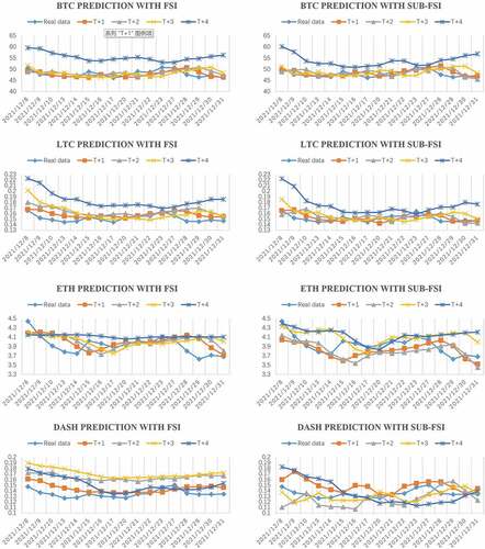
This article conducts a further check of the performance of the GNN with FSI and with sub-FSI by comparing the forecast results of the two strategies among prediction steps of +1 day, +2 days, +3 days, and +4 days. The results are shown in Figure A2. When focusing on the similarity, it is clear that GNN with sub-FSI provides better performance in forecasting BTC and LTC. Meanwhile, GNN with FSI gives better prediction to ETH and DASH. These results show that the GNN strategy with the lowest MAE and RMSE cannot guarantee the best forecasting in every node of the graph. This gives a hint that the whole graph prediction has this weakness. Each graph in our article has its own advantages. Viewing from finance theory, the prediction differences may reveal the heterogeneity in market efficiency among cryptocurrencies, which is consistent with the findings of Naeem et al. (2021). Specifically, BTC was classified as ‘speculative’ and ‘diversification’ asset, while ETH was treated as ‘professional’ and ‘complementary’ based on the analysis of tail risk measurement (Ahelegbey, Giudici, and Mojtahedi 2021). Considering that BTC is the most important node with the highest price and trading volume in the graph, it can be seen that the GNN with sub-FSI method has overall better performance in the predictions of +1 day, +2 days, +3 days, and +4 days.

Figure A2: Comparison of the predicted prices of the cryptocurrencies between with FSI and sub-FSI.

6. Sensitivity analysis with GNN

To verify the effectiveness of the strategy used in this article, Table A6 provides a sensitivity analysis with GNN. It is clear that the prediction accuracy of the method drops significantly when FSI or sub-FSI are excluded from the embedding graph. These findings further show that the variable USDT should be included when forecasting the price of these four cryptocurrencies with GNN. It should also be noted that the GNN method gives much worse forecasting results when variables FSI/sub-FSI and USDT are excluded from the graph, especially when making long prediction steps.

Table A6. Sensitivity check of excluding the FSI and USDT.

		GNN without FSI/sub-FSI	GNN without USDT		GNN without FSI/sub-FSI and USDT
			with FSI	with sub-FSI
+1 day	MAE	0.338	0.375	0.693	1.342
	MAPE	0.064	0.097	0.160	0.123
	RMSE	0.863	0.756	0.998	1.850
+2 days	MAE	0.509	0.495	1.574	1.778
	MAPE	0.101	0.102	0.212	0.123
	RMSE	1.313	1.025	4.086	3.426
+3 days	MAE	0.625	0.485	1.230	1.999
	MAPE	0.093	0.112	0.174	0.155
	RMSE	1.678	1.001	3.207	3.936
+4 days	MAE	0.904	0.563	0.497	3.592
	MAPE	0.138	0.132	0.189	0.201
	RMSE	2.170	1.189	1.326	6.748
+5 days	MAE	1.037	0.645	2.062	3.408
	MAPE	0.124	0.115	0.281	0.190
	RMSE	2.391	1.603	5.217	6.533
+6 days	MAE	0.844	0.627	2.253	2.962
	MAPE	0.112	0.135	0.291	0.193
	RMSE	2.116	1.546	5.605	5.641
+7 days	MAE	1.040	0.653	2.199	2.480
	MAPE	0.099	0.152	0.334	0.173
	RMSE	2.378	1.539	5.518	4.675

References

- Ahelegbey, D. F., M. Billio, and R. Casarin. 2016. “Bayesian Graphical Models for Structural Vector Autoregressive Processes.” Journal of Applied Econometrics 31 (2): 357–386. doi:10.1002/jae.2443.
- Ahelegbey, D. F., P. Giudici, and F. Mojtahedi. 2021. “Tail Risk Measurement in Crypto Assets Markets.” International Review of Financial Analysis 73: 101604. doi:10.1016/j.irfa.2020.101604.
- Billio, M., M. Getmansky, A. W. Lo, and L. Pelizzon. 2012. “Econometric Measures of Connectedness and Systemic Risk in the Finance and Insurance Sectors.” Journal of Financial Economics 104 (3): 535–559. doi:10.1016/j.jfineco.2011.12.010.
- Bouri, E., R. Gupta, C. K. M. Lau, and D. Roubaud. 2021. “Risk Aversion and Bitcoin Returns in Extreme Quantiles.” Economics Bulletin 41 (3): 1374–1386.
- Bouri, E., R. Gupta, C. K. M. Lau, D. Roubaud, and S. Wang. 2018. “Bitcoin and Global Financial Stress: A Copula-Based Approach to Dependence and Causality in the Quantiles.” The Quarterly Review of Economics and Finance 69: 297–307. doi:10.1016/j.qref.2018.04.003.
- Cheng, D. W., F. Z. Yang, S. Xiang, and J. Liu. 2022. “Financial Time Series Forecasting with Multi-Modality Graph Neural Network.” Pattern Recognition 121: 108218. doi:10.1016/j.patcog.2021.108218.
- Diebold, F. X., and K. Yilmaz. 2009. “Measuring Financial Asset Return and Volatility Spillovers, with Application to Global Equity Markets.” The Economic Journal 119 (534): 158–171. doi:10.1111/j.1468-0297.2008.02208.x.
- Giudici, P., and I. Abu-Hashish. 2019. “What Determines Bitcoin Exchange Prices? A Network VAR Approach.” Finance Research Letters 28: 309–318. doi:10.1016/j.frl.2018.05.013.
- Giudici, P., and P. Pagnottoni. 2019. “High Frequency Price Change Spillovers in Bitcoin Exchange Markets.” Risks 7 (4): 111. doi:10.3390/risks7040111.
- Giudici, P., and P. Pagnottoni. 2020. “Vector Error Correction Models to Measure Connectedness of Bitcoin Exchange Markets.” Applied Stochastic Models in Business and Industry 36 (1): 95–109. doi:10.1002/asmb.2478.
- Giudici, P., and G. Polinesi. 2021. “Crypto Price Discovery Through Correlation Networks.” Annals of Operations Research 299 (1–2): 443–457. doi:10.1007/s10479-019-03282-3.
- Kim, T., and H. Y. Kim. 2019. “Forecasting Stock Prices with a Feature Fusion LSTM-CNN Model Using Different Representations of the Same Data.” PLOS One 14 (2): e0212320. doi:10.1371/journal.pone.0212320.
- Lewenfus, G., W. A. Martins, S. Chatzinotas, and B. Ottersten. 2020. “Joint Forecasting and Interpolation of Time-Varying Graph Signals Using Deep Learning.” IEEE Transactions on Signal and Information Processing Over Networks 6: 761–773. doi:10.1109/TSIPN.2020.3040042.
- Liu, Q. F., Z. Y. Tao, Y. M. Tse, and C. J. Wang. 2021. “Stock Market Prediction with Deep Learning: The Case of China.” Financial Research Letters 46 (A): 102209. doi:10.1016/j.frl.2021.102209.
- Lu, Z. L., W. F. Lv, Y. B. Cao, Z. P. Xie, H. Peng, and B. Du. 2020. “LSTM Variants Meet Graph Neural Networks for Road Speed Prediction.” Neurocomputing 400: 34–45. doi:10.1016/j.neucom.2020.03.031.
- Naeem, M. A., E. Bouri, Z. Peng, S. J. H. Shahzad, and X. V. Vo. 2021. “Asymmetric Efficiency of Cryptocurrencies During COVID19.” Physica A: Statistical Mechanics and Its Applications 565: 125562. doi:10.1016/j.physa.2020.125562.
- Smyl, S. 2020. “A Hybrid Method of Exponential Smoothing and Recurrent Neural Networks for Time Series Forecasting.” International Journal of Forecasting 36 (1): 75–85. doi:10.1016/j.ijforecast.2019.03.017.
- Wang, L., P. K. Sarker, and E. Bouri. 2022. ”Short- and Long-Term Interactions Between Bitcoin and Economic Variables: Evidence from the US.” Computational Economics, forthcoming. doi:10.1007/s10614-022-10247-5.
- Wei, W. Q., Q. Zhang, and L. Liu. 2021. “Bitcoin Transaction Forecasting with Deep Network Representation Learning.” IEEE Transactions on Emerging Topics in Computing 9 (3): 1359–1371. doi:10.1109/TETC.2020.3010464.
- Wen, Z., E. Bouri, Y. Xu, and Y. Zhao. 2022. “Intraday Return Predictability in the Cryptocurrency Markets: Momentum, Reversal, or Both.” North American Journal of Economics and Finance 62: 101733. doi:10.1016/j.najef.2022.101733.
- Yu, B., H. Yin, and Z. Zhang. 2018. ”Spatio-Temporal Graph Convolutional Networks: A Deep Learning Framework for Traffic Forecasting.” In: Twenty-Seventh International Joint Conference on Artificial Intelligence IJCAI-18. doi: 10.24963/ijcai.2018/505.