Numerical Ross Recovery for Diffusion Processes Using a PDE Approach

ABSTRACT

We develop and analyse a numerical method for solving the Ross recovery problem for a diffusion problem with unbounded support, with a transition independent pricing kernel. Asset prices are assumed to only be available on a bounded subinterval $B=[-N,N]$. Theoretical error bounds on the recovered pricing kernel are derived, relating the convergence rate as a function of $N$ to the rate of mean reversion of the diffusion process. Our suggested numerical method for finding the pricing kernel employs finite differences, and we apply Sturm–Liouville theory to make use of inverse iteration on the resulting discretized eigenvalue problem. We numerically verify the derived error bounds on a test bench of three model problems.

KEYWORDS:

• Ross recovery
• diffusion process
• numerical method

1. Introduction

A fundamental question in financial markets is to what extent asset prices may be used to infer the market participants’ views about the likelihood for different events, e.g. the risk of a stock market crash. The traditional view has been that because investors are risk averse and therefore require a premium above expected returns when purchasing an asset, only limited inferences may be drawn about such likelihoods. Indeed, what is observed is actually a risk neutral expectation – a combination of a pricing kernel and the true expectation. Ross (2015), however, shows that under some circumstances it is actually possible to recover both the pricing kernel and true probabilities from observed prices. Such Ross recovery, when possible, provides important information about the market.

Several papers study the theoretical conditions under which Ross recovery is possible, see, Carr and Yu (2012), Park (2016), Qin and Linetsky (2016), Walden (2017) and Jensen, Lando, and Pedersen (2019), extending Ross’s original approach in various directions.¹ A more empirically oriented literature focuses on whether Ross recovery works in practice, with mixed results, see Borovička, Hansen, and Scheinkman (2016), Audrino, Huitema, and Ludwig (2014), Tran and Xia (2014), Bakshi, Chabo-Yo, and Gao (2018), Massacci, Williams, and Zhang (2016), Backwell (2015), and Schneider and Trojani (2016).

An interesting case when Ross recovery works is in a complete market, where the process governing asset payoffs is a diffusion that satisfies certain growth conditions, and the pricing kernel is transition independent, as discussed in Walden (2017). This setting arises in many work-horse models in finance. The pricing kernel can in this case be recovered as the maximal positive eigenfunction to a second-order elliptic differential operator, a problem that is related to Sturm–Liouville theory.

The theoretical conditions needed for perfect recovery are not satisfied in practice. With a diffusion process governing the state space, an infinite number of assets in the market would be needed. In practice, even when derivative markets are included, only a finite number are available. There will therefore be gaps between observed prices and upper and lower bounds on these observations. In this paper, we study the numerical challenges that arise in such a context, with a focus on the boundedness of observations.

We focus on the case when the state space is governed by a diffusion process and the pricing kernel is transition independent, but asset prices are only available on a bounded subinterval symmetric around the origin, $B=[-N,N]$, with no given boundary condition. We denote this the approximate recovery problem. For simplicity, we assume that all asset prices are available within this interval – i.e. that there are no gaps – and focus on the boundedness of the domain.

Our contribution is two-fold. First, we derive error bounds on the recovered pricing kernel – as characterized by the representative agent’s marginal utility function and personal discount rate – that depend on the underlying parameters of the model. Briefly, the more mean reverting the process is, the faster is the convergence in $N$. Our key result on these error bounds is presented in Proposition 3.1. We numerically verify for several test problems that the actual approximation error is in line with these theoretical bounds.

Second, we introduce a numerical method. Our key result here is Proposition 4.1, which allows us to rewrite the approximate recovery problem as a solution to a regular Sturm–Liouville problem on the interval $[-N,N]$, in turn leading to the finite difference algorithm for solving the problem, which we introduce in Section 6. The method addresses the challenge that one must simultaneously solve for the marginal utility function and the largest eigenvalue that admits positivity. Overall, our paper takes a step towards making Ross recovery for diffusion processes practically operational.

2. The approximate Ross recovery problem

The Ross recovery problem for a univariate time homogeneous diffusion process can via the Kolmogorov equations be transformed into the following ODE problem on the real line

(1) $D{z}^{\prime \prime }+\kappa z^{\prime }+(\rho -r)z=0.$(1)

This ODE is derived in Walden (2017), in an economy with a complete financial market for state contingent claims and an underlying time-homogeneous diffusion process, $X_t$, with dynamics

$d{X}_t=\mu (X_t)dt+\sigma (X_t)d\omega ,t\ge 0.$

Here, $D(x)={\sigma }^2(x)/2,$ $\kappa (x)$, and $r(x)$ are known functions that we assume are smooth, and such that $\sigma$ is uniformly bounded above 0, $\sigma (x)\ge ϵ>0$ for all $x\in \mathbb{R}$. The derivation of (1) is based on arbitrage theory. Specifically, the function $\kappa (x)$ represents the risk-neutral drift term of the $X_t$ process, whereas the $\sigma$ function represents the volatility of the process. The process $r$ represents the short-term risk free rate in the economy, the constant $\rho$ represents a representative investor’s personal discount rate and the function $z$ is the reciprocal of the agent’s so-called marginal utility function, $z=1/m$. This is standard setting for dynamic equilibrium asset pricing models in continuous time. We refer to Walden (2017) for further details.

Only strictly positive solutions $z(x)$ to (1) are considered.² The constant $\rho$ is not observed, and neither is the function $z(x)$. The Ross recovery problem in this context is that of identifying $\rho$ and $z(x)$, given $D(x)$, $\kappa (x)$, and $r(x)$. The function $z(x)$ is only unique down to multiplication with an arbitrary positive constant. In what follows, we therefore always normalize $z(x)$ and assume that $z(0)=1$.

Define the operator ${\mathcal{L}}_{\lambda }[z]=D{z}^{\prime \prime }+\kappa z^{\prime }+(\lambda -r)z$, and the fundamental ODE for the recovery problem

(2) ${\mathcal{L}}_{\lambda }[z]=0,\lambda \in \mathbb{R}.$(2)

The correct $z$ is then a strictly positive solution to the fundamental ODE with the parameter value $\lambda =\rho$. For a given $\lambda$ and a positive solution $w$ to (2), a candidate solution is represented by the pair $\theta$ $=(\lambda ,w)$. Define the sets

$\begin{array}{ccc}W& \stackrel{\mathrm{d}\mathrm{e}\mathrm{f}}{=}& \left\{w:w(x)>0\right\},\\ \mathrm{\Theta }& \stackrel{\mathrm{d}\mathrm{e}\mathrm{f}}{=}& \left\{\left(\lambda ,w\right):{\mathcal{L}}_{\lambda }[w]=0\mathrm{a}\mathrm{n}\mathrm{d}w\in W\right\},\\ \mathrm{\Lambda }& \stackrel{\mathrm{d}\mathrm{e}\mathrm{f}}{=}& \{\lambda :(\lambda ,w)\in \mathrm{\Theta }\}.\end{array}$

Also define the number $\bar{\lambda }=sup\mathrm{\Lambda }\in [\rho ,\mathrm{\infty }).$ Given that $\bar{\lambda }$ is finite, call solutions on the form $(\bar{\lambda },w)$ maximal. The Ross recovery problem can now be restated as that of identifying a maximal $\theta \in \mathrm{\Theta }$.

The functions $\mu (x)=\kappa (x)+2D(x)\frac{z^{\prime }(x)}{z(x)}$ and $D(x)$ determine whether Ross recovery is feasible.³ We define

$Q(x)=e^{-{\int }_0^x\frac{\mu (s)}{D(s)}ds},$

$R(x)={\int }_0^{x}Q(s)ds,$

$T(x)=min\{-R(-x),R(x)\},$

$Z(x,N)=min\left\{\frac{R(N)}{R(x)},\frac{R(-N)}{R(-x)}\right\},$

and note that $R(x)$ is a smooth, strictly positive, and increasing function, as is $T(x)$ on the positive axis, and that $R(x)=x(1+o(x))$ for small $x$.

A necessary and sufficient condition for Ross recovery to be feasible is that ${lim}_{x\to \mathrm{\infty }}T(x)=\mathrm{\infty }$. We have

Proposition 2.1. If ${lim}_{x\to \mathrm{\infty }}T(x)=\mathrm{\infty }$, then there is a unique maximal solution to (2), $(\bar{\lambda },w)\in \mathrm{\Theta }$, that solves the Ross recovery problem, $\rho =\bar{\lambda }$ and $z=w$. If ${lim}_{x\to \mathrm{\infty }}T(x)<\mathrm{\infty }$, then there are distinct positive solutions to (2), ${\theta }_1=(\rho ,w_1)\in \mathrm{\Theta }$, and ${\theta }_2=(\rho ,w_2)\in \mathrm{\Theta }$, and Ross recovery is therefore not possible.

We refer to Walden (2017) (see also Borovička, Hansen, and Scheinkman (2016) and Qin and Linetsky (2016)) for a proof of Proposition 2.1. In light of this result we focus our analysis on the case ${lim}_{x\to \mathrm{\infty }}T(x)=\mathrm{\infty }$ going forward. It follows that in this case ${lim}_{N\to \mathrm{\infty }}Z(x,N)=\mathrm{\infty }$ for all $x\ne 0$.

The functions $D(x)$, $\kappa (x)$, and $r(x)$ need to be backed out from the market prices, and in practice such prices cannot be observed for arbitrarily large $x$. In other words, the problem needs to be truncated. As discussed in Walden (2017), when the functions are only observed on some compact subdomain of $\mathbb{R}$ – for simplicity, we assume on a symmetric interval around the origin, $x\in B\stackrel{\mathrm{d}\mathrm{e}\mathrm{f}}{=}[-N,N]$, $0<N<\mathrm{\infty }$ – it is possible to find approximations to $\rho$ and $z$ by solving the problem on this subdomain. Specifically, define

$\begin{array}{ccc}{W}^N& \stackrel{\mathrm{d}\mathrm{e}\mathrm{f}}{=}& \left\{w^N:w^N(x)>0\mathrm{f}\mathrm{o}\mathrm{r}x\in (-N,N)\right\},\\ {\mathrm{\Theta }}^N& \stackrel{\mathrm{d}\mathrm{e}\mathrm{f}}{=}& \left\{\left({\lambda }^N,w^N\right):{\mathcal{L}}_{{\lambda }^N}[w^N]=0\mathrm{f}\mathrm{o}\mathrm{r}x\in [-N,N]\mathrm{a}\mathrm{n}\mathrm{d}{w}^N\in W^N\right\},\\ {\mathrm{\Lambda }}^N& \stackrel{\mathrm{d}\mathrm{e}\mathrm{f}}{=}& \{{\lambda }^N:({\lambda }^N,w^N)\in {\mathrm{\Theta }}^N\}.\end{array}$

and ${\bar{\lambda }}^N=sup{\mathrm{\Lambda }}^N.$ Obviously, the set ${\mathrm{\Theta }}^N$ shrinks as $N$ grows, and $\mathrm{\Theta }\subset {\mathrm{\Theta }}^N$ for all finite $N$. It is easy to see that ${\mathrm{\Lambda }}^N$ is closed and bounded above for all $N>0$.⁴ The approximate solution to the Ross recovery problem is now chosen as a maximal element in ${\mathrm{\Theta }}^N$, ${\theta }^N=({\bar{\lambda }}^N,z^N)\in {\mathrm{\Theta }}^N$. We denote the problem of finding such a maximal element, the approximate recovery problem, ARP.

It is shown in Walden (2017) that ${\theta }^N$ converges to $\theta$ as $N$ tends to infinity, but the speed of convergence is not analysed. Neither is the question of how to jointly solve for ${\bar{\lambda }}^N$ and $z^N$ in an efficient manner. We mainly focus on these questions in our subsequent analysis.

3. Convergence analysis

Our main convergence result is the following:

Proposition 3.1. The approximation errors between the approximate recovered and true solutions, ${\theta }^N=({\bar{\lambda }}^N,z^N)$ and $\theta =(\rho ,z)$, satisfy the following bounds.

(3) $0\le {\bar{\lambda }}^N-\rho \le C_1\frac{1}{T(N)-ϵ},$(3)

(4) $\left|\frac{z^N(x)-z(x)}{z(x)}\right|\le C_2\frac{1}{Z(x,N)-1}.$(4)

Here, the positive constant $C_1$ depends on $\mu$ and $\sigma$, and on $ϵ>0$, and the positive constant $C_2$ depends on $\mu$, $\sigma$, and $x$, but neither constant depends on $N$.

Proof. We know that $\mathrm{\Theta }\subset {\mathrm{\Theta }}^N$, and for finite $N$ we in general expect there to be solutions outside of $\mathrm{\Theta }$, on the form $(\rho +a,z^N)\in {\mathrm{\Theta }}^N$ with $a>0$. We write any such solution as $z^N(x)=e^{-{\int }_0^x\frac{\mu (s)}{{\sigma }^2(s)}ds}{g}_a(x)z(x)$, where $g_a$ satisfies the following ODE on normal form (see Simmons (1988))

(5) $g_a^{{ }^{\prime \prime }}+\left(\frac{a}{D}-\frac{1}{4}{\left(\frac{\mu }{D}\right)}^2-\frac{1}{2}\frac{d}{dx}\left(\frac{\mu }{D}\right)\right)g_a=0,$(5)

and we note that positivity of $z^N$ is equivalent to positivity of $g_a$. In general, there may be multiple positive solutions to (5) for a specific $a$. For $a=0$, we identify the solution $g_0=e^{{\int }_0^x\frac{\mu (s)}{{\sigma }^2(s)}ds},$ which leads to $z^N=z$. We refer to Walden (2017) for a detailed explanation of the argument.

For $a>0$, we focus on the solution $g_a$, such that $g_a(0)=1$, $g_a^{\prime }(0)=g_0^{\prime }(0)=\frac{\mu (0)}{{\sigma }^2(0)}$. As we shall see, the analysis of this particular solution of (5) will help us understand the general solution.

It is easy to see that for any $x>0$, such that $g_a(x)>0$, the function $\mathrm{\Gamma }(x)\stackrel{\mathrm{d}\mathrm{e}\mathrm{f}}{=}\frac{g_{0^{\prime }}(x)}{g_0(x)}-\frac{g_{a^{\prime }}(x)}{g_a(x)}$ satisfies the nonlinear equation

(6a) ${\mathrm{\Gamma }}^{\prime }={\mathrm{\Gamma }}^2-\frac{\mu }{D}\mathrm{\Gamma }+\frac{a}{D},$(6a)

(6b) $\mathrm{\Gamma }(0)=0,$(6b)

and that at the smallest $x_0>0$ for which $g_a(x_0)=0$ (there must of course exist such a point if $a>0$, since no positive solutions exist for $a>0$; moreover, as shown in the proof of Proposition 2 in Walden (2017), there exists at least one positive and one negative such point), $\mathrm{\Gamma }(x)\nearrow \mathrm{\infty }$ as $x\nearrow x_0$, i.e. $\mathrm{\Gamma }$ blows up at $x_0$.

We want to find a lower bound on $x_0$, given $a>0$. Clearly, $x_0$ increases towards infinity as $a$ decreases towards 0, because of the continuous dependence of solutions to the ODE (1) on its parameters. We assume that $a$ is sufficiently small so that $x_0>1$, and note that $\mathrm{\Gamma }(x)>0$ for all $x>0$, since if $\mathrm{\Gamma }(x)$ approaches 0, then the term $\frac{a}{D}$ on the right-hand-side of (6a) dominates the others.

Define the constants $\eta ={min}_{0\le x\le 1}\frac{1}{D(x)}$, and $\xi =max\{0,{max}_{0\le x\le 1}\frac{\mu (x)}{D(x)}\}$. A standard differential inequality implies that if $\hat{\mathrm{\Gamma }}$ solves

(7a) ${\hat{\mathrm{\Gamma }}}^{\prime }=-\xi \hat{\mathrm{\Gamma }}+\eta a,$(7a)

(7b) $\hat{\mathrm{\Gamma }}(0)=0,$(7b)

then $\mathrm{\Gamma }\ge \hat{\mathrm{\Gamma }}$ for all $0<x\le 1$. The solution to (7a,b) when $\xi >0$ is $\hat{\mathrm{\Gamma }}(u)=\frac{\eta (1-e^{-\xi u})}{\xi }a\ge \frac{\eta }{2}au\stackrel{\mathrm{d}\mathrm{e}\mathrm{f}}{=}{\hat{C}}_{1}au$ for $0\le u\le min\{1,\frac{1}{\xi }\}$, and thus $\mathrm{\Gamma }(u)\ge \hat{\mathrm{\Gamma }}(u)\ge {\hat{C}}_{1}au$, for such $u$. The inequality $\hat{\mathrm{\Gamma }}(u)\ge {\hat{C}}_{1}au$ also trivially holds for all $u$ when $\xi =0$, since $\hat{\mathrm{\Gamma }}(u)=\eta au\ge {\hat{C}}_{1}au$ in this case. A similar argument is made in Walden (2017).

We choose a small fixed strictly positive $u$, $0\le u\le min\{1,\frac{1}{\xi }\}$, and next study the Bernoulli equation

(8a) $Y^{\prime }=Y^2-\frac{\mu }{D}Y,$(8a)

(8b) $Y(u)={\hat{C}}_{1}au,$(8b)

for $x\ge u$, and note that another differential inequality implies that $\mathrm{\Gamma }(x)\ge Y(x)$ for $u\le x\le x_0$, so if $Y$ blows up at $x_1$, then $x_0\le x_1$. Rewriting (8a) as

$-\frac{\mu }{D}=\frac{Y^{\prime }}{Y}-Y,$

integrating both sides between $u$ and $p$, $u\le p\le x$, we get

$-{\int }_u^p\frac{\mu (s)}{D(s)}ds={\left[ln(Y(s))\right]}_u^p-{\int }_u^{p}Y(s)ds,$

which when taking the exponential and multiplying by $Y(u)$ leads to

(9) $Y(u)e^{{\int }_0^u\frac{\mu (s)}{D(s)}ds}Q(p)=Y(p)e^{-{\int }_u^{p}Y(s)ds}=-\frac{d}{dp}{e}^{-{\int }_u^{p}Y(s)ds}.$(9)

Finally, integrating both sides of (9) between $u$ and $x$, leads us to

$Y(u)e^{{\int }_0^u\frac{\mu (s)}{D(s)}ds}\left(R(x)-R(u)\right)=1-e^{-{\int }_u^{x}Y(s)ds},$

implying that $Y(x)$ blows up when

$Y(u)e^{{\int }_0^u\frac{\mu (s)}{D(s)}ds}\left(R(x)-R(u)\right)\nearrow 1,$

i.e. since $u$ is small, before $x$ grows to the point where

$\frac{1}{2}{\hat{C}}_{1}au\left(R(x)-u\right)=1,$

which corresponds to

(10) $a=\frac{2}{{\hat{C}}_{1}u}\times \frac{1}{R(x)-u}.$(10)

By an identical argument for $x<0$, it follows that a negative $v$ close to 0, and a constant ${\hat{C}}_2>0$, can be defined such that $\mathrm{\Gamma }(x)\to -\mathrm{\infty }$ before $x$ reaches the point where

$\frac{1}{2}{\hat{C}}_{2}a|v|\left(-R(x)-|\upsilon |\right)=1,$

which corresponds to

$a=\frac{2}{{\hat{C}}_2|\upsilon |}\times \frac{1}{-R(x)-|\upsilon |}.$

Altogether, we have shown that $\mathrm{\Gamma }(x)$ blows up to both negative and positive infinity within the interval

$x\in B=\left\{N:|N|\le \frac{C_1}{T(N)-ϵ}\right\},$

where $C_1=max\{2{\hat{C}}_1/ϵ,2{\hat{C}}_2/ϵ\},$ $ϵ=min\{u,|\upsilon |\}$. Thus, $g_a$ has two roots in $B$, and does therefore not belong to ${\mathrm{\Theta }}^N$. Moreover, the Sturm separation theorem implies that any solution to (5) (not just the one with the initial conditions studied so far) has at least one root in $B$, and therefore does not belong to ${\mathrm{\Theta }}^N$ either. This leads to the necessary condition for the existence of a solution $z^N$, which is positive in $[-N,N]$:

(11) $a\le max\left\{\frac{C_1}{R(N)-ϵ},\frac{C_1}{-R(-N)-ϵ}\right\}$(11)

which is equivalent to (3).

Thus, to recap, we have shown that if $a$ does not satisfy at least one of the conditions:

(12a) $a\ge C_1\frac{1}{R(N)-ϵ},$(12a)

(12b) $a\ge C_1\frac{1}{-R(-N)-ϵ},$(12b)

then any candidate $z^N$ must have at least one root in $[-N,N]$, and thus be disqualified as a candidate solution to the approximate recovery problem.

Note that the constant $C_1$ increases in $ϵ$, which in turn depends on how $u$ and $v$ are chosen.

For inequality (4), we note that

$\left|\frac{z^N(x)-z(x)}{z(x)}\right|=\left|\frac{g_a(x)-g_0(x)}{g_0(x)}\right|=\left|\frac{g_a(x)}{g_0(x)}-1\right|,$

where $g_a$ is a solution to (5) that satisfies $g_a(0)=1$. It follows that $\mathrm{\Gamma }(x)=\frac{g_0^{\prime }(x)}{g_0(x)}-\frac{g_a^{\prime }(x)}{g_a(x)}$ satisfies

${\mathrm{\Gamma }}^{\prime }={\mathrm{\Gamma }}^2-\frac{\mu }{D}\mathrm{\Gamma }+\frac{a}{D},$

$\mathrm{\Gamma }(0)=\upsilon ,$

for some $\upsilon$, which we without loss of generality assume is weakly positive, and that $\mathrm{\Gamma }$ is defined on the interval $B=(-N,N)$ if $z^N>0$ on that interval.

It is easy to verify that

(13) $\frac{g_a(x)}{g_0(x)}=e^{-{\int }_0^x\mathrm{\Gamma }(s)ds},$(13)

and moreover, a similar argument as that for $a$ above implies that the solution $Y(x)$ to the ODE

(14a) $Y^{\prime }=Y^2-\frac{\mu }{D}Y,$(14a)

(14b) $Y(y)=\mathrm{\Gamma }(y),0<y<x,$(14b)

satisfies $Y(s)\le \mathrm{\Gamma }(s)$, $y<s<N$, and does therefore not blow up before $N$.

The solution to (14a,b) satisfies

$e^{-{\int }_y^{N}Y(s)ds}=1-\mathrm{\Gamma }(y)e^{{\int }_0^y\frac{\mu (s)}{D(s)}ds}(R(N)-R(y))\ge 0,$

so, for $y>0$,

$\mathrm{\Gamma }(y)\le \frac{e^{-{\int }_0^y\frac{\mu (s)}{D(s)}ds}}{R(N)-R(x)}=\frac{Q(y)}{R(N)-R(x)}.$

It follows from (13) that, for $x>0$,

$\begin{array}{rl}& \left|\frac{z^N(x)-z(x)}{z(x)}\right|\le 1-e^{-{\int }_0^{x}Q(y)dy/(R(N)-R(x))}\\ & \le 1-e^{-1/(Z(x,N)-1)}\\ & =O\left(\frac{1}{Z(x,N)-1}\right),\end{array}$

where the rightmost equality follows from a Taylor expansion of the exponential function and the fact that for large $N$, $Z(x,N)$ tends to infinity regardless of $x$.

An identical argument shows that the inequality also holds for $x<0$ (letting $N\to -\mathrm{\infty })$. We are done. □

Proposition 3.1 implies standard convergence orders, depending on the behaviour of the function $R$. For example the following result is an immediate consequence of the proposition when $R(x)$ is a regularly varying function (see Feller 1971).

Corollary 3.2. If $R(x)$ is a regularly varying function, i.e. if $\frac{R(kx)}{R(x)}\sim k^{\nu }$ for some constant $\nu >0$ for large $k$, then for a fixed $x$,

(15) $|{\bar{\lambda }}^N-\rho |=O(N^{-\nu }),\left|\frac{z^N(x)-z(x)}{z(x)}\right|=O\left(N^{-\nu }\right).$(15)

We note that ${\bar{\lambda }}^N>\rho$, so the approximation error is one-sided with respect to $\rho$ in the corollary.

An important variable with significant economic meaning is the representative agent’s risk aversion: $G(x)=-\frac{(1/z{)}^{\prime }}{(1/z)}=-\frac{-z^{\prime }}{z^2(1/z)}=\frac{z^{\prime }(x)}{z(x)}$,⁵ which in our truncated problem is approximated by $G^N(x)=\frac{(z^N{)}^{\prime }(x)}{z^N(x)}$. The approximation error of the risk aversion is thus $e^N(x)=\left|G(x)-G^N(x)\right|$, which we will also study.

4. A regular Sturm–Liouville problem

It is convenient to reformulate the approximate recovery problem as a regular Sturm–Liouville problem. That this is possible is a consequence of the following result:

Proposition 4.1. The solution to the approximate recovery problem is zero at both boundaries, $z^N(-N)=z^N(N)=0$.

Proof. We first note that since we focus on the case when recovery on the real line is possible, i.e. on the case for which ${lim}_{x\to \mathrm{\infty }}T(x)=\mathrm{\infty }$, existence of a positive solution to the fundamental ODE for $\lambda =\rho$ is guaranteed and, moreover, any solution for $\lambda >\rho$ will eventually become negative. This follows from the analysis in Walden (2017).

Assume that ${\theta }^N=({\bar{\lambda }}^N,z^N)$ solves the approximate recovery problem. If $z^N>0$ for all $x\in [-N,N]$, then a standard perturbation argument implies that there is an element $(\bar{\lambda }+ϵ,{\hat{z}}^N)\in {\mathrm{\Theta }}^N$ for some small $ϵ>0$, and ${\theta }^N$ is therefore not maximal, leading to a contradiction. Thus, $z^N$ is zero in at least one of the boundaries, $x=\pm N$.

Without loss of generality, assume that $z^N(-N)=0$. If $z^N(N)=0$ we are done, so assume that $z^N(x)>0$, for $x\in (-N,N]$ (recall that $z^N(x)>0$ in $x\in (-N,N)$, since ${\theta }^N\in {\mathrm{\Theta }}^N$). From the theory of second-order linear ODEs, it follows that there exists another nontrivial solution, ${\tilde{z}}^N$, to the fundamental ODE ${\mathcal{L}}_{\bar{\lambda }}[z]=0$. Clearly, it cannot be the case that ${\tilde{z}}^N$ is positive for all $x\in [-N,N)$, since then it would follow that $({\bar{\lambda }}^N,z^N+{\tilde{z}}^N)\in {\mathrm{\Theta }}^N$, and the same argument as before would imply that ${\theta }^N$ is not maximal. Similarly, ${\tilde{z}}^N$ cannot be negative for all $x\in [-N,N)$.

So, ${\tilde{z}}^N$ has at least one root in $[-N,N)$, and by the Sturm separation theorem, it must have exactly one root in $(-N,N)$. Without loss of generality, assume that ${\tilde{z}}^N(-N)>0$ and ${\tilde{z}}^N(N)\le 0$. For small enough $\epsilon >0$, it follows that ${\hat{z}}^N=z^N+ϵ{\tilde{z}}^N$ is strictly positive on $[-N,N]$, and also that $({\bar{\lambda }}^N,{\hat{z}}^N)\in {\mathrm{\Theta }}^N$, again implying that ${\theta }^N$ is not maximal.

So, for ${\theta }^N$ to be maximal it must be that $z^N(-N)=z^N(N)=0$. We are done. □

Proposition 4.1 immediately leads to an equivalent formulation of the approximate recovery problem as a regular Sturm–Liouville problem:

(16) $\begin{array}{ccc}-D{(w^N)}^{{ }^{\prime \prime }}-\kappa {(w^N)}^{\prime }+r{w}^N& =& {\lambda }^N{w}^N,\\ w^N(-N)& =& 0,\\ w^N(N)& =& 0.\end{array}$(16)

Specifically, from Sturm–Liouville theory, it follows that (21) has a discrete set of solutions, with associated eigenvalues, ${\lambda }^N={\lambda }_1^N<{\lambda }_2^N<{\lambda }_3^N<\dots <{\lambda }_n^N<\dots$, and eigenfunctions, $w_1^N,w_2^N,\dots w_n^N,\dots$, where $w_n^N$ has $n-1$ zeros on $(-N,N)$. Hence, the solution to the approximate recovery problem is the smallest eigenvalue and associated eigenfunction to the Sturm–Liouville problem (16), ${\theta }^N=\left({\bar{\lambda }}^N,z^N\right)=\left({\lambda }_1^N,w_1^N\right)$.

Our approach in the next section is to use inverse iterations to solve a discretized version of the ODE (21), using the finite difference method, and thereby differs from other suggested approaches. The risk-neutral distribution can be estimated from observed option prices, see Breeden and Litzenberger (1978), Jackwerth and Rubinstein (1996), Dupire (1994), and Ross (2015). Ross (2015) assumes a discrete, finite, state space, under which exact recovery is possible by solving a recursive system of equations. The approach uses Perron-Frobenius theory for (finite dimensional) nonnegative matrices, and therefore does not address the issue of truncation when the state space is unbounded. Carr and Yu (2012) solve the fundamental ODE (1) on an interval under the assumption of Robin boundary conditions, allowing for perfect recovery in this case. As noted in Dubynskiy and Goldstein (2013), however, the specification of the boundary condition has a significant effect on the recovered solution. The truncation issue is therefore present also with their approach.

Park (2016), also using a PDE approach, studies the extension of the recovery to transient processes. These processes will violate the condition ${lim}_{x\to \mathrm{\infty }}T(x)=\mathrm{\infty }$ in Proposition 2.1. In this case, recovery is impossible without further knowledge about $\rho$. When $\rho$ is known and additional conditions are satisfied, recovery is also possible for this case with $T(\mathrm{\infty })<\mathrm{\infty }$, see Park (2016). The numerical analysis of ARP for this case is an interesting potential extension.

Other papers focus directly on the link between risk-neutral and physical probabilities, avoiding the PDE formulation. Jackwerth and Menner (2017) apply Ross’s discrete model to S&P 500 call option data, and find that recovered distributions are incompatible with physical probabilities. Similarly, Dillschneider and Maurer (2018), also using S&P options pricing data and assuming a bounded state space, find empirical evidence that the pricing kernel is misspecified under this approach. Our PDE approach complement these papers, by focusing on the numerical implications of truncating the state space. A general implication of our analysis is that the rate of mean reversion of the physical process influences the numerical challenges associated with empirical recovery. This relation may provide a clue about why the results from the empirical recovery literature have been mixed so far, although other explanations are also possible, e.g. misspecification.

5. Analysis of model problems

We define three model problems that will serve as a test bench.

5.1. Model problem 1 – Ornstein–Uhlenbeck process

The Ross recovery problem for an Ornstein–Uhlenbeck process with the pricing kernel determined by power preferences is $\mu (x)=-\beta x$, $\beta >0$, $\sigma (x)=\sigma$, $z(x)=e^{\gamma x}$, $r(x)=\text{break}\rho -\gamma \beta x-\frac{{\gamma }^2{\sigma }^2}{2}$, $\kappa (x)=-\beta x-\gamma {\sigma }^2$. The risk aversion in this case is thus $G(x)\equiv \gamma$. The underlying stochastic process is

$d{X}_t=-\beta X_{t}dt+\sigma d\omega ,t\ge 0.$

Since the sign of the drift term (the $dt$ term) is negative and grows in $X_t$ whereas the coefficient for the volatility term (the $d\omega$ term) is constant, this process is mean reverting. In fact, when $X_t$ is far away from the origin, which is its long term mean, it will quickly revert back towards this mean with high probability (see Oksendahl 1998).

We choose the parameters $\beta =0.05$, $\sigma =0.2$, and $\rho =0.02$. We use $\gamma =2$ in the numerical experiments and analyse a problem with $\gamma =0$.

For this problem, we have $Q(x)=e^{\frac{\beta }{{\sigma }^2}{x}^2}$ which gives

$R(x)={\int }_0^{x}Q(s)ds={\int }_0^x{e}^{\frac{\beta }{{\sigma }^2}{s}^2}ds=\frac{\sqrt{\pi }{\mathrm{e}\mathrm{r}\mathrm{f}\mathrm{i}}_{\left(\sqrt{\frac{\beta }{{\sigma }^2}}x\right)}}{2\sqrt{\frac{\beta }{{\sigma }^2}}},$

and since ${\mathrm{e}\mathrm{r}\mathrm{f}\mathrm{i}}_{(}x)=-\mathrm{e}\mathrm{r}\mathrm{f}\mathrm{i}(-x)$ we get $T(x)=\frac{\sqrt{\pi }\left|\mathrm{e}\mathrm{r}\mathrm{f}\mathrm{i}\left(\sqrt{\frac{\beta }{{\sigma }^2}}x\right)\right|}{2\sqrt{\frac{\beta }{{\sigma }^2}}}$, and finally $Z(x,N)=$ $\left|\frac{\mathrm{e}\mathrm{r}\mathrm{f}\mathrm{i}\left(\sqrt{\frac{\beta }{{\sigma }^2}}N\right)}{\mathrm{e}\mathrm{r}\mathrm{f}\mathrm{i}\left(\sqrt{\frac{\beta }{{\sigma }^2}}x\right)}\right|$. This means that $T(N)$ and $Z(x,N)$ grow extremely fast, and we correspondingly expect fast, super-exponential, convergence as $N$ grows.

5.2. Exact solution with $\gamma =0$

When $\gamma =0$, we can derive an exact solution to the approximate recovery problem. Equation (21)(21) $x_{\left[n\right]}=x(x+1)(x+2)\cdots (x+n-1).$(21) with $\sigma (x)=\sigma$, $\mu (x)=-\beta x$, $r=\rho$ is given by

(17) $\begin{array}{ccc}-\frac{{\sigma }^2}{2}{(z^N)}^{{ }^{\prime \prime }}+\beta x{(z^N)}^{\prime }+\rho z^N& =& {\bar{\lambda }}^{N}z,\\ z^N(0)& =& 1,\\ z^N(N)& =& 0,\end{array}$(17)

with analytical solution

(18) $z^N(x)=c_1\frac{e^{\frac{\beta }{2{\sigma }^2}{x}^2}wM\left(-\frac{2{\bar{\lambda }}^N-2\rho +\beta }{4\beta },-\frac{1}{4},-\frac{\beta }{{\sigma }^2}{x}^2\right)}{\sqrt{x}}+c_2\frac{e^{\frac{\beta }{2{\sigma }^2}{x}^2}wW\left(-\frac{2{\bar{\lambda }}^N-2\rho +\beta }{4\beta },-\frac{1}{4},-\frac{\beta }{{\sigma }^2}{x}^2\right)}{\sqrt{x}}.$(18)

Here $wM$ and $wW$ are Whittaker functions defined by

(19) $\begin{array}{ccc}wM(k,m,y)& =& y^{1/2+m}{e}^{-y/2}M(m-k+\frac{1}{2},1+2m,y),\\ wW(k,m,y)& =& y^{1/2+m}{e}^{-y/2}U(m-k+\frac{1}{2},1+2m,y),\end{array}$(19)

where $M$ and $U$ are Kummer’s functions defined by

(20) $\begin{array}{c}M(a,b,y)={\sum }_{n=0}^{\mathrm{\infty }}\frac{a_{\left[n\right]}}{n!b_{\left[n\right]}}{y}^n,\\ U(a,b,y)=\frac{\mathrm{\Gamma }(1-b)}{\mathrm{\Gamma }(a-b+1)}M(a,b,y)+\frac{\mathrm{\Gamma }(b-1)}{\mathrm{\Gamma }(a)}{y}^{1-b}M(a-b+1,2-b,y),\end{array}$(20)

and $x_{\left[n\right]}$ denotes the Pochhammer symbol defined by

(21) $x_{\left[n\right]}=x(x+1)(x+2)\cdots (x+n-1).$(21)

Inserting (20) and (19) in (18) gives

(22) $\begin{array}{rl}& z^N(x)=e^{\frac{\beta }{{\sigma }^2}{x}^2}{\left(-\frac{\beta }{{\sigma }^2}\right)}^{1/4}\left(c_{1}M\left(\frac{{\bar{\lambda }}^N-\rho +\beta }{2\beta },\frac{1}{2},-\frac{\beta }{{\sigma }^2}{x}^2\right)\right.\\ & +c_2\left(\frac{\mathrm{\Gamma }(\frac{1}{2})}{\mathrm{\Gamma }(\frac{{\bar{\lambda }}^N-\rho +2\beta }{2\beta })}M\left(\frac{{\bar{\lambda }}^N-\rho +\beta }{2\beta },\frac{1}{2},-\frac{\beta }{{\sigma }^2}{x}^2\right)\right.\\ & \left.\left.+i\cdot \frac{\mathrm{\Gamma }(-\frac{1}{2})}{\mathrm{\Gamma }(\frac{{\bar{\lambda }}^N-\rho +\beta }{2\beta })}{\left(\frac{\beta }{{\sigma }^2}{x}^2\right)}^{1/2}M\left(\frac{{\bar{\lambda }}^N-\rho +2\beta }{2\beta },\frac{3}{2},-\frac{\beta }{{\sigma }^2}{x}^2\right)\right)\right)\end{array}$(22)

The unknown coefficients $c_1$ and $c_2$ as well as ${\bar{\lambda }}^N$ are determined by the boundary conditions

(23) $\begin{array}{ccc}{z}^N(0)& =& 1,\\ z^N(N)& =& 0,\end{array}$(23)

together with the fact that we are looking for real-valued solutions $({\bar{\lambda }}^N,z^N)$. The latter condition gives that $c_2=0$ since $M(a,b,y)$ is real for all values of $a$, $b$, and $y$. Since

$\underset{x\to 0}{lim}M\left(\frac{{\bar{\lambda }}^N-\rho +\beta }{2\beta },\frac{1}{2},-\frac{\beta }{{\sigma }^2}{x}^2\right)=1$

we get from the boundary condition in $x=0$ that $(-\frac{\beta }{{\sigma }^2}{)}^{1/4}{c}_1=1.$ Thus, the solution is given by

(24) $z^N(x)=e^{\frac{\beta }{{\sigma }^2}{x}^2}M\left(\frac{{\bar{\lambda }}^N-\rho +\beta }{2\beta },\frac{1}{2},-\frac{\beta }{{\sigma }^2}{x}^2\right).$(24)

Finally, ${\bar{\lambda }}^N$ is determined from the boundary condition in $x=N$, i.e.

(25) $M\left(\frac{{\bar{\lambda }}^N-\rho +\beta }{2\beta },\frac{1}{2},-\frac{\beta }{{\sigma }^2}{N}^2\right)=0,$(25)

is solved for ${\bar{\lambda }}^N$.

We verify the high convergence rate of ${\bar{\lambda }}^N$ to $\rho$ in the following proposition

Proposition 5.1. Equation (25)(25) $M\left(\frac{{\bar{\lambda }}^N-\rho +\beta }{2\beta },\frac{1}{2},-\frac{\beta }{{\sigma }^2}{N}^2\right)=0,$(25) implies the following error bound:

$|{\bar{\lambda }}^N-\rho |\le CN{e}^{-\frac{\beta }{{\sigma }^2}{N}^2},$

where the constant $C$ does not depend on $N$.

Proof. Define $\delta =\frac{{\bar{\lambda }}^N-\rho }{2\beta }$, and ${\tau }^2=\frac{\beta }{{\sigma }^2}{N}^2$. We then have that

(26) $M\left(\delta +\frac{1}{2},\frac{1}{2},-{\tau }^2\right)=0,$(26)

so if we show that for large $\tau$, the $\delta$ for which (26) holds satisfies $\delta \le C_0\tau e^{-{\tau }^2}$, Proposition 5.1 follows, since

$|{\bar{\lambda }}^N-\rho |=2\beta \delta \le 2\beta C_0\tau e^{-{\tau }^2}=C_0\frac{2{\beta }^{3/2}}{\sqrt{{\sigma }^2}}N{e}^{-\frac{\beta }{{\sigma }^2}{N}^2}=CN{e}^{-\frac{\beta }{{\sigma }^2}{N}^2}.$

It follows from standard properties of the Kummer function that there is exactly one strictly positive solution to (31), in $\tau$, for each $\delta >0$, and that

$M\left(\delta +\frac{1}{2},\frac{1}{2},-{\tau }^2\right)=\frac{{\tau }^{\frac{1}{2}}}{\mathrm{\Gamma }(1/2+\delta )}{\int }_0^{\mathrm{\infty }}{e}^{-t}{t}^{\delta -\frac{1}{4}}\sqrt{\frac{2}{\pi }}\frac{cos(2\sqrt{t}\tau )}{\sqrt{2\sqrt{t}\tau }}dt=\frac{1}{\mathrm{\Gamma }(1/2+\delta )}{\int }_0^{\mathrm{\infty }}{e}^{-\frac{x^2}{4{\tau }^2}}{\left(\frac{x}{2\tau }\right)}^{2\delta }\sqrt{\frac{1}{\pi }}cos(x)\frac{1}{2\tau }dx$

where we substituted $\sqrt{t}$ for $\frac{x}{2\tau }$ in the integration. To prove the theorem, we study how fast $\delta$ tends to zero as $\tau$ tends to infinity.

Defining

$H(\tau ,\delta ,a,b)={\int }_a^b{e}^{-\frac{x^2}{4{\tau }^2}}{x}^{2\delta }cos(x)dx,$

and $H(\tau ,\delta )=H(\tau ,\delta ,0,\mathrm{\infty })$, the $\delta$ that satisfies (26) – as a function of $\tau$ – per definition satisfies $H(\tau ,\delta )=0.$

Now, $H(\tau ,0)={\int }_0^{\mathrm{\infty }}{e}^{-\frac{x^2}{{\tau }^2}}dx=\sqrt{\pi }\tau e^{-{\tau }^2}>0$, and $H$ is continuous in $\delta$ so $H(\tau ,0+)>0$. Therefore, if $H(\tau ,\hat{\delta })\le 0$ then $\delta \le \hat{\delta }$.

We have

$H(\tau ,\hat{\delta })=H(\tau ,0)+H(\tau ,\hat{\delta })-H(\tau ,0)=\sqrt{\pi }\tau e^{-{\tau }^2}+{\int }_0^{\mathrm{\infty }}V(x)cos(x)dx,$

where $V(x)=e^{-\frac{x^2}{4{\tau }^2}}(x^{2\hat{\delta }}-1)$. So, to summarize, if for a large $\tau$, and a small $\hat{\delta }>0$, the inequality

${\int }_0^{\mathrm{\infty }}V(x)cos(x)dx\le -\sqrt{\pi }\tau e^{-{\tau }^2}$

holds, it follows that $\delta \le \hat{\delta }$.

For positive $\hat{\delta }$, the (continuous) function $V(x)$ is obviously negative for sufficiently small positive $x$, positive for sufficiently large $x$, and ${lim}_{x\to \mathrm{\infty }}V(x)=0$. So it has at least one local maximum. Moreover,

$V^{\prime }(x)=e^{-\frac{x^2}{4{\hat{\tau }}^2}}\left(-\frac{x}{2{\hat{\tau }}^2}(x^{2\hat{\delta }}-1)+2\hat{\delta }{x}^{2\hat{\delta }-1}\right)=\frac{e^{-\frac{x^2}{4{\hat{\tau }}^2}}x}{2{\hat{\tau }}^2}L(x),$

where

(27) $L(x)=-x^{2\hat{\delta }}+4\hat{\delta }{\tau }^2{x}^{2\hat{\delta }-2}+1.$(27)

It follows that $V^{\prime }(x)$ is positive for small positive $x$, so $V(x)$ is increasing close to the origin.

At a local extremum of $V$, $x^{\ast }$, $L(x^{\ast })=0$, and since $L^{\prime }(x)=-2\hat{\delta }{x}^{2\delta -1}-2\hat{\delta }(2-\text{break}2\hat{\delta })x^{2\hat{\delta }-3}$, which is negative for all positive $x$ (since $\hat{\delta }$ is close to zero), $L(x)$ is decreasing in $x$. The function $V$ thus has at most one interior extremum. So, $V$ – which is initially increasing and eventually decreasing – must have exactly one strict local maximum that occurs at $x^{\ast }$, which is also the function’s global maximum.

It is easy to see that $L(1)>0$, so it follows that $x^{\ast }>1$. Using the substitution $x=e^w$, rewriting (27) as $1=e^{2\hat{\delta }w}-4\hat{\delta }{\tau }^2{e}^{2(\hat{\delta }-2)w}$, and Taylor expanding the r.h.s. around $\hat{\delta }=0$ yields

$1=1+(2w-4e^{-2w}{\tau }^2)\hat{\delta }+(2w^2-8e^{-2w}w{\tau }^2){\hat{\delta }}^2+O({\hat{\delta }}^3),$

which leads to

$\tau =\frac{1}{\sqrt{2}}{x}^{\ast }\sqrt{log(x^{\ast })}(1+o(\hat{\delta })).$

Thus, the growth in $x^{\ast }$ is a bit slower than linear as $\tau$ grows and, since we are focusing on $\hat{\delta }$ extremely close to zero, $\hat{\delta }\sim \tau e^{-{\tau }^2}$, the impact of $\hat{\delta }$ on $x^{\ast }$ is negligible.

For a given $\tau$, define the integer $m$, such that $\pi /2+2m\pi <x^{\ast }\le \pi /2+(2m+2)\pi$. We decompose the integral into the sum of four sub-integrals:

$\begin{array}{l}{\int }_0^{\infty }V(x)\cos (x)dx={\int }_0^{3\pi /2}V(x)\cos (x)dx+{\int }_{3\pi /2}^{\pi /2+2m\pi }V(x)\cos (x)dx\\ +{\int }_{\pi /2+2m\pi }^{7\pi /2+2m\pi }V(x)\cos (x)dx+{\int }_{7\pi /2+2m\pi }^{\infty }V(x)\cos (x)dx.\end{array}$

Note that for the second and fourth terms we have

${\int }_{3\pi /2}^{\pi /2+2m\pi }V(x)cos(x)dx\le 0,$

since $V(x)$ is increasing on $[3\pi /2,\pi /2+2m\pi ]$, and

${\int }_{7\pi /2+2m\pi }^{\mathrm{\infty }}V(x)cos(x)dx\le 0,$

since $V(x)$ is decreasing on $[7\pi /2+2m\pi ,\mathrm{\infty })$.

For the first term, we get

${\int }_0^{3\pi /2}V(x)cos(x)dx\le {\int }_0^{\pi /2}V(x)cos(x)dx={\int }_0^{\pi /2}{e}^{-\frac{x^2}{4{\tau }^2}}(x^{2\hat{\delta }}-1)cos(x)dx\le \frac{1}{2}{\int }_0^1(x^{2\hat{\delta }}-1)dx+\frac{5}{9}{\int }_1^{\pi /2}(x^{2\hat{\delta }}-1)dx=\frac{1}{2}\left(\frac{1}{1+2\hat{\delta }}-1\right)+\frac{5}{18}\left(2-\pi +\frac{4^{-\hat{\delta }}{\pi }^{1+2\hat{\delta }}}{1+2\hat{\delta }}\right)=\frac{1}{18}(2-10\pi -5\pi log(4)+10\pi log(\pi ))\hat{\delta }+O({\hat{\delta }}^2)=-0.85\hat{\delta }+O({\hat{\delta }}^2).$

Here, we used the inequalities $\frac{1}{2}<cos(1)<\frac{5}{9}$ on the third line of the above inequality. Finally, a Taylor expansion around $\hat{\delta }=0$ of the third term yields

${\int }_{\pi /2+2m\pi }^{7\pi /2+2m\pi }V(x)cos(x)dx\le \frac{6\pi }{log(log(\sqrt{log(1/\hat{\delta })}))}\times \hat{\delta }+O({\hat{\delta }}^2)\le 0.35\hat{\delta },$

for sufficiently small $\hat{\delta }$.

Altogether, we therefore arrive at

$H(\tau ,\hat{\delta })=\sqrt{\pi }\tau e^{-{\tau }^2}+{\int }_0^{\mathrm{\infty }}V(x)cos(x)dx,\le \sqrt{\pi }\tau e^{-{\tau }^2}-0.85\hat{\delta }+0.35\hat{\delta }\le 0,$

for large $\tau$, when $\hat{\delta }=2\sqrt{\pi }\tau e^{-{\tau }^2}$ is chosen. The result thus follows, with $C=2\sqrt{\pi }$, in line with the earlier argument. □

5.3. Model problem 2 – Algebraic rate of convergence

The functions $\mu (x)=\frac{\beta }{2}(1-\alpha )x$, $\alpha >0$, $\beta >0$, and $\sigma (x)=\sqrt{\beta (1+x^2)}$, corresponding to the underlying stochastic process

$d{X}_t=\frac{\beta }{2}(1-\alpha )X_{t}dt+\sqrt{\beta (1+X_t^2)}d\omega ,t\ge 0.$

For $\alpha >1$, the drift term pulls $X_t$ back towards zero (because $1-\alpha <0$, so the sign of the drift term is opposite of the sign of the process). The larger $\alpha$ is, the stronger is this effect. The volatility term randomly counterweights this pull towards zero and, in contrast to the Ornstein–Uhlenbeck process, grows with the size of $X_t$. This process will therefore tend to spend much time far away from its long-term mean, especially for low $\alpha$ which corresponds to a low impact by the drift term on the process.

The specification leads to $Q(x)=(1+x^2{)}^{\frac{\alpha -1}{2}}$, which implies $R(x)=xF([\frac{1}{2},-\frac{\alpha -1}{2}],\text{break}\frac{3}{2},-x^2)$ where $F(a,b,y)={\sum }_{k=0}^{\mathrm{\infty }}\left(\frac{{(a_1)}_{[k]}{(a_2)}_{[k]}\cdots {(a_p)}_{[k]}}{{(b_1)}_{[k]}{(b_2)}_{[k]}\cdots {(b_q)}_{[k]}}\right)\left(\frac{y^k}{k!}\right)$ is the generalized hypergeometric function, where $a=(a_1,\dots ,a_p)$, $b=(b_1,\dots ,b_q)$, and $x_{\left[n\right]}$ denotes the Pochhammer symbol defined in (26). This gives $T(N)=NF([\frac{1}{2},-\frac{\alpha -1}{2}],\frac{3}{2},-N^2)$ and finally $Z(x,N)=\frac{NF([\frac{1}{2},-\frac{\alpha -1}{2}],\frac{3}{2},-N^2)}{xF([\frac{1}{2},-\frac{\alpha -1}{2}],\frac{3}{2},-x^2)}$. Since $Q(x)\approx x^{\alpha -1}$ for large $x$ we get $R(x)\approx \frac{x^{\alpha }}{\alpha }$, i.e. the convergence behaviour for large $N$ is approximately given by $T(N)=\frac{N^{\alpha }}{\alpha }$ and $Z(x,N)={\left(\frac{N}{x}\right)}^{\alpha }$. Hence, from Corollary 3.2 we expect the convergence rate to be of order $\alpha$, i.e. the convergence rate to be algebraic in contrast to the superexponential convergence rate in the previous problem.

We have $z(x)=e^{\gamma x}$, $\gamma =2$, $r(x)=\rho +\gamma \frac{\beta }{2}(1-\alpha )x-\frac{{\gamma }^2}{2}\beta (1+x^2)$, $\kappa (x)=\frac{\beta }{2}(1-\alpha )\text{break}x-\gamma \beta (1+x^2)$, and we choose $\beta =0.04$, $\rho =0.02$, and $\gamma =2$.

5.4. Model problem 3 – Higher dimensions

In higher dimensions, the Ross recovery problem leads to an elliptic PDE. An example is given in Walden (2017) for the two-dimensional diffusion process

$dX=-\beta Ydt+{\sigma }_{x}d{w}_X,$

$dY=-Ydt+{\sigma }_{y}d{w}_Y,$

with $z(x,y)=e^{\gamma x}$. The recovery argument in this case leads to the following two-dimensional PDE:

(28) $\frac{{\sigma }_x^2}{2}{z}_{xx}+\frac{{\sigma }_y^2}{2}{z}_{yy}-y{z}_y-(\beta y+\gamma {\sigma }_x^2)z_x+\left(\lambda -r\right)z=0,$(28)

with $r(x,y)=\rho -\gamma \beta y-{\gamma }^2\frac{{\sigma }_x^2}{2}$. The parameters are $\gamma =2$, $\rho =0.02$, ${\sigma }_x=0.2$, ${\sigma }_y=0.5$, $\beta =0.1$. As discussed in Walden (2017), the solution technique yields a unique solution in this case too.

6. Numerical method

We discretize (16) using centred finite differences on a uniform grid $x_j=-N+(j-1)\cdot \mathrm{\Delta }x$, $j=1,\dots ,2M_x+1$, $\mathrm{\Delta }x=N/M_x$:

(29) $\begin{array}{rl}& -D_j\frac{w_{j+1}^N-2w_j^N+w_{j-1}^N}{\mathrm{\Delta }{x}^2}-{\kappa }_j\frac{w_{j+1}^N-w_{j-1}^N}{2\mathrm{\Delta }x}+r_j{w}_j^N={\lambda }^N{w}_j^N\\ & j=2,\dots ,2M_x,\\ & w_1^N=0,\\ & w_{2M_x+1}^N=0,\end{array}$(29)

where $w_j^N\approx w^N(x_j)$. Equation (29)(29) $\begin{array}{rl}& -D_j\frac{w_{j+1}^N-2w_j^N+w_{j-1}^N}{\mathrm{\Delta }{x}^2}-{\kappa }_j\frac{w_{j+1}^N-w_{j-1}^N}{2\mathrm{\Delta }x}+r_j{w}_j^N={\lambda }^N{w}_j^N\\ & j=2,\dots ,2M_x,\\ & w_1^N=0,\\ & w_{2M_x+1}^N=0,\end{array}$(29) can be written as

(30) $A{w}^N={\lambda }^N{w}^N,$(30)

where $w^N={\left(w_2^N,\dots ,w_{2M_x}^N\right)}^T$.

For the two-dimensional problem (28) we also introduce $y_k=-N+(k-1)\cdot \mathrm{\Delta }y$, $k=1,\dots ,2M_y+1$, $\mathrm{\Delta }y=N/M_y$ and discretize

(31) $\begin{array}{c}-\frac{{\sigma }_x^2}{2}\cdot \frac{w_{j+1,k}^N-2w_{j,k}^N+w_{j-1,k}^N}{\mathrm{\Delta }{x}^2}-\frac{{\sigma }_y^2}{2}\cdot \frac{w_{j,k+1}^N-2w_{j,k}^N+w_{j,k-1}^N}{\mathrm{\Delta }{y}^2}+\\ \hspace{0.17em}\\ y_k\cdot \frac{w_{j,k+1}^N-w_{j,k-1}^N}{2\mathrm{\Delta }y}+(\beta y_k+\gamma {\sigma }_x^2)\cdot \frac{w_{j+1,k}^N-w_{j-1,k}^N}{2\mathrm{\Delta }x}+r{w}_{j,k}^N={\lambda }^N{w}_{j,k}^N,\\ \hspace{0.17em}\\ j=2,\dots ,2M_x,k=2,\dots ,2M_y,\\ \hspace{0.17em}\\ w_{1,k}^N=w_{2M_x+1,k}^N=0,k=1,\dots ,2M_y+1,\\ \hspace{0.17em}\\ w_{j,1}^N=w_{j,2M_y+1,k}^N=0,j=1,\dots ,2M_x+1,\end{array}$(31)

where $w_{j,k}^N\approx w^N(x_j,y_k)$. Now (31) can be written as (30) with

$w^N={\left(w_{2,2}^N,\dots ,w_{2M_x,2}^N,w_{2,3}^N,\dots ,w_{2M_x,2M_y}^N\right)}^T.$

We want to find the smallest eigenvalue ${\bar{\lambda }}^N$ to (35). Since ${\bar{\lambda }}^N>\rho >0$, this is also the eigenvalue to (35) with the smallest magnitude. Hence, we can use inverse iteration to compute ${\theta }^N=({\bar{\lambda }}^N,z^N)$ where $z^N$ is the eigenvector to (35) corresponding to the smallest eigenvalue ${\bar{\lambda }}^N$.

Algorithm 1 Inverse iteration

Choose $z^{N,0}$.

for $\mathrm{\ell }=0,\dots ,$ until convergence do

Solve $A{q}^{\mathrm{\ell }+1}=z^{N,\mathrm{\ell }},$

$z^{N,\mathrm{\ell }+1}=\frac{q^{\mathrm{\ell }+1}}{\parallel q^{\mathrm{\ell }+1}\parallel },$

${\bar{\lambda }}^{N,\mathrm{\ell }+1}=\frac{{(z^{N,\mathrm{\ell }+1})}^{T}A{z}^{N,\mathrm{\ell }+1}}{{(z^{N,\mathrm{\ell }+1})}^T{z}^{N,\mathrm{\ell }+1}},$

The matrix $A$ is $LU$-factorized prior to the loop over $\mathrm{\ell }$ and the factors are then used in the solution of $A{q}^{\mathrm{\ell }+1}=LU{q}^{\mathrm{\ell }+1}=z^{\mathrm{\ell }}$. As convergence criterion we use

(32) $|{\bar{\lambda }}^{N,\mathrm{\ell }+1}-{\bar{\lambda }}^{N,\mathrm{\ell }}|\le ϵ.$(32)

In all numerical experiments in Section 7 we use $\epsilon ={10}^{-6}$.

Since the solution $z^N$ only is determined up to a multiplicative constant, we scale the obtained solution $z^N$ from Algorithm 1 such that the final solution fulfils $z^N(0)=z(0)$.

7. Numerical results

In Figure 1, we show $z^N(x)$ for Model problems 1, 2 (with $\alpha =2$ and $\alpha =5$), and 3 with $\gamma =2$, together with $z(x)$. The corresponding values of ${\bar{\lambda }}^N$ are given in the legends. We use the numerical method described in Section 6 to compute $z^N(x)$. For Model problems 1 and 2, we use discretization parameter $\mathrm{\Delta }x={10}^{-3}$ and for Model problem 4 we use discretization parameters $\mathrm{\Delta }x=2\cdot {10}^{-2}$ and $\mathrm{\Delta }y=2\cdot {10}^{-2}$.

Figure 1. Plots of $z^N(x)$ for $N=2$, 2.5, and 3 together with $z(x)=e^{\gamma x}$ for $\gamma =2$. The corresponding values of ${\bar{\lambda }}^N$ are given in the legends.

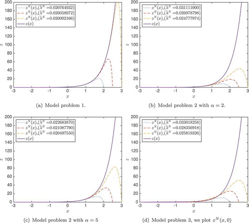
From Figure 1, it is clear that for Model problem 1 the convergence is very fast in $N$. For Model problem 2 we have faster convergence in $N$ for larger $\alpha$ as expected from the theory.

In Figure 2, we display $\frac{{\bar{\lambda }}^N-\rho }{\rho }$, $\frac{|z^N(1)-z(1)|}{z(1)}$ and $\frac{|G^N(1)-G(1)|}{G(1)}$ as a function of $N$ for Model problems 1, 2 (with $\alpha =2$ and $\alpha =5$), and 3 using $\gamma =2$. We have used the discretization parameters in Table 1 that are chosen such that the discretization error in (34) is negligible compared to the approximation errors between the approximate recovered and true solutions. In the same figure, we show the theoretical error as a function of $N$ originating from $N=2$. We conjecture that the convergence rate for $G^N$ is the same as for $z^N$, and therefore compare the actual convergence rate for $G^N$ with the theoretical convergence rate for $z^N$.

Table 1. Discretization parameters.

MP 1	$\mathrm{\Delta }x={10}^{-5}$
MP 2	$\mathrm{\Delta }x={10}^{-4}$
MP 3	$\mathrm{\Delta }x=2\cdot {10}^{-2}$, $\mathrm{\Delta }y={10}^{-2}$

Figure 2. Convergence plots for MP 1, 2 (with $\alpha =2$ and $\alpha =5$), and 3.

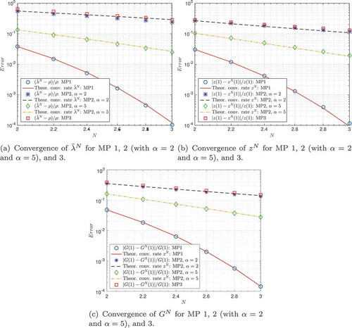
In Table 2, we compare theoretical and actual convergence rates.

Table 2. Convergence rate.

	Theoretical (upper limit of) damping of relative error between $N=2$ and $N=3$			Actual damping of relative error in computed solution between $N=2$ and $N=3$			Actual damping/theoretical damping
	${\bar{\lambda }}^N$	$z^N$	$G^N$	${\bar{\lambda }}^N$	$z^N$	$G^N$	${\bar{\lambda }}^N$	$z^N$	$G^N$
MP1	3.18 × 10^−3	3.03 × 10^−3	3.03 × 10^−3	2.73 × 10^−3	3.79 × 10^−3	3.00 × 10^−3	0.86	1.25	0.99
MP2, $\alpha =2$	5.23 × 10^−1	4.02 × 10^−1	4.02 × 10^−1	4.30 × 10^−1	4.39 × 10^−1	3.71 × 10^−1	0.82	1.09	0.92
MP2, $\alpha =5$	1.97 × 10^−1	1.75 × 10^−1	1.75 × 10^−1	1.85 × 10^−1	1.87 × 10^−1	1.71 × 10^−1	0.93	1.07	0.98

From Figure 2 and Table 2, we conclude that the convergence behaviour for Model problems 1–2 agrees very well with the theory. Finally, we note that the two-dimensional Model problem 3 converges approximately as Model problem 2 with $\alpha =2$.

In Table 3, we display the number of iterations in Algorithm 1 to reach the convergence criterion (37) for $\epsilon ={10}^{-6}$. We have used the discretization parameters in Table 1.

Table 3. Number of iterations.

$N$	MP1	MP2, $\alpha =2$	MP2, $\alpha =5$	MP3
2.0	10	11	9	15
2.2	11	11	9	16
2.4	11	11	9	17
2.6	11	11	9	18
2.8	11	11	9	20
3.0	11	12	9	21

From Table 3, we conclude that the number of iterations to reach convergence is relatively low and does not increase much with problem size.

8. Conclusions

In this paper, we consider Ross recovery when the state space is governed by a diffusion process with support on the whole real line, the pricing kernel is transition independent, and asset prices are only available on a bounded subinterval, $B=[-N,N]$, of the state space. We denote this the approximate recovery problem, ARP. We show that the solution to this problem is zero at both boundaries $x=-N$ and $x=N$ and hence can be written as a regular Sturm–Liouville problem. We derive theoretical error bounds on the recovered pricing kernel that depend on the underlying parameters of the model, and show that the more mean reverting the process is, the faster is the convergence when $N$ increases.

We introduce a finite difference method to solve the ARP, which results in a discretized eigenvalue problem. Using Sturm–Liouville theory we find the solution of the ARP as given by the smallest eigenvalue of a standard finite difference matrix, and its associated eigenfunction. Hence, we can use inverse iteration to obtain the solution.

A test bench of three model problems are defined and analysed, and we verify the theoretical error bounds for these problems. Moreover, the tests show that a numerically accurate solution is obtained in relatively few iterations by our algorithm. Our approach takes a step towards making Ross recovery for diffusion processes practically operational.

Acknowledgments

The authors are grateful to professor emeritus Bertil Gustafsson for valuable discussions about the content of this paper. We are especially thankful for his sharing of expertise in the numerical solution of and boundary conditions for ordinary differential equations. We also thank two anonymous referees for many constructive comments and suggestions that have helped improve the paper.

Disclosure statement

No potential conflict of interest was reported by the authors.

Notes

1. See also Alvarez and Jerman (2005), Hansen and Scheinkman (2009), Hansen (2012), and Hansen and Scheinkman (2013) for papers further related to Ross’s approach.

2. In the economic formulation of the problem, $z$ is the reciprocal of the so-called marginal utility function of the economy’s representative agent, $z=1/m$. It follows from first principles of economics that the marginal utility function is always strictly positive.

3. Note that the formulation in Walden (2017) is $\kappa (x)=\mu (x)+2D(x)\frac{m^{\prime }(x)}{m(x)}$, which is consistent with our formulation because $z=1/m$.

4. So, we could equivalently have defined ${\bar{\lambda }}^N=max{\mathrm{\Lambda }}^N$.

5. Specifically, if the agent’s consumption is defined by $e^x$, $G(x)$ corresponds to the so-called coefficient of relative risk aversion, whereas if the agent’s consumption is $x$, $G(x)$ corresponds to the coefficient of absolute risk aversion. Both measures are important in understanding attitudes towards risk in an economy.

References

- Alvarez, F., and J. Jerman. 2005. “Using Asset Prices to Measure the Persistence of the Marginal Utility of Wealth.” Econometrica 73: 1977–2016. doi:10.1111/ecta.2005.73.issue-6.
- Audrino, F., R. Huitema, and M. Ludwig. 2014. “An Empirical Analysis of the Ross Recovery Theorem.” Working Paper, University of Zurich.
- Backwell, A. 2015. “State Prices and Implementation of the Recovery Theorem.” Journal of Risk and Financial Management 8: 2–16. doi:10.3390/jrfm8010002.
- Bakshi, G., F. Chabo-Yo, and X. Gao. 2018. “A Recovery that We Can Trust? Deducing and Testing the Restrictions of the Recovery Theorem.” Review of Financial Studies 31: 532–555.
- Breeden, D. T., and R. H. Litzenberger. 1978. “Prices of State-contingent Claims Implicit in Option Prices.” Journal of Business. 621–651. doi:10.1086/296025.
- Carr, P., and J. Yu. 2012. “Risk, Return, and Ross Recovery.” Journal of Derivatives 20: 38–59. doi:10.3905/jod.2012.20.1.038.
- Dillschneider, Y., and R. Maurer. 2018. “Functional Ross Recovery: Theoretical Results and Empirical Tests.” Working Paper, Goethe University.
- Dubynskiy, A., and R. S. Goldstein. 2013. “Recovering Drifts and Preference Parameters from Financial Derivatives.” Working Paper, University of Minnesota.
- Dupire, B. 1994. “Pricing with a Smile.” Risk 7: 18–20.
- Feller, W. 1971. An Introduction to Probability Theory and Its Applications. New York: Wiley.
- Hansen, L. P. 2012. “Dynamic Valuation Decomposition Within Stochastic Economies.” Econometrica 80: 911–987.
- Hansen, L. P., and J. A. Scheinkman. 2009. “Long-term Risk: An Operator Approach.” Econometrica 77: 177–234.
- Hansen, L. P., and J. A. Scheinkman. 2013. “Stochastic Compounding and Uncertain Valuation.” Working Paper, Princeton University.
- Jackwerth, J. C., and M. Menner. 2017. “Does the Ross Recovery Theorem Work Empirically.” Working Paper, University of Konstanz.
- Jackwerth, J. C., and M. Rubinstein. 1996. “Recovering Probability Distributions from Option Prices.” Journal of Finance 51: 1611–1631. doi:10.1111/j.1540-6261.1996.tb05219.x.
- Jensen, C. S., D. Lando, and L. H. Pedersen. 2019. “Generalized Recovery.” Journal of Financial Economics 133: 154–174.
- Massacci, F., J. Williams, and Y. Zhang. 2016. “Empirical Recovery: Hansen-Scheinkman Factorization and Ross Recovery from High Frequency Option Prices.” Working Paper, Durham University.
- Oksendahl, B. 1998. Stochastic Differential Equations. Springer-Verlag.
- Park, H. 2016. “Ross Recovery with Recurrent and Transient Processes.” Quantitative Finance 16: 667–676. doi:10.1080/14697688.2015.1092572.
- Qin, L., and V. Linetsky. 2016. “Positive Eigenfunctions of Markovian Pricing Operators: Hansen-Scheinkman Factorization, Ross Recovery, and Long-Term Pricing.” Operations Reseach 64: 99–117.
- Borovička, J., L. P. Hansen, and J. A. Scheinkman. 2016. “Misspecified Recovery”. Journal of Finance 71: 2493–2544. Forthcoming. doi:10.1111/jofi.2016.71.issue-6.
- Ross, S. 2015. “The Recovery Theorem.” Journal of Finance 70: 615–648. doi:10.1111/jofi.12092.
- Schneider, P., and F. Trojani. 2016. “(Almost) Model-Free Recovery.” Journal of Finance. Forthcoming.
- Simmons, G. 1988. Differential Equations. New York: McGraw Hill.
- Tran, N.-K., and S. Xia. 2014. “Specificed Recovery.” Working Paper, Olin Business School.
- Walden, J. 2017. “Recovery with Unbounded Diffusion Processes.” Review of Finance 21: 1403–1444. doi:10.1093/rof/rfw068.