Unbiased Deep Solvers for Linear Parametric PDEs

Abstract

We develop several deep learning algorithms for approximating families of parametric PDE solutions. The proposed algorithms approximate solutions together with their gradients, which in the context of mathematical finance means that the derivative prices and hedging strategies are computed simultaneously. Having approximated the gradient of the solution, one can combine it with a Monte Carlo simulation to remove the bias in the deep network approximation of the PDE solution (derivative price). This is achieved by leveraging the Martingale Representation Theorem and combining the Monte Carlo simulation with the neural network. The resulting algorithm is robust with respect to the quality of the neural network approximation and consequently can be used as a black box in case only limited a-priori information about the underlying problem is available. We believe this is important as neural network-based algorithms often require fair amount of tuning to produce satisfactory results. The methods are empirically shown to work for high-dimensional problems (e.g., 100 dimensions). We provide diagnostics that shed light on appropriate network architectures.

Keywords:

• Monte Carlo method
• deep neural network
• control variates
• partial differential equations

2010 Mathematics Subject Classifications:

• 65M75
• 60H30
• 91G60

1. Introduction

Numerical algorithms that solve PDEs suffer from the so-called ‘curse of dimensionality’, making it impractical to apply known discretization algorithms such as finite difference schemes to solve high-dimensional PDEs. However, it has been recently shown that deep neural networks trained with stochastic gradient descent can overcome the curse of dimensionality (Beck, Gonon, and Jentzen 2020; Berner, Grohs, and Jentzen 2020), making them a popular choice to solve this computational challenge in the last few years.

In this work, we focus on the problem of numerically solving parametric linear PDEs arising from European option pricing in high dimensions. Let $B\subseteq {\mathbb{R}}^p,p\ge 1$ be a parameter space (for instance, in the Black–Scholes equation with fixed rate, B is the domain of the volatility parameter). Consider $v=v(t,x;\text{β})$ satisfying (1) $\begin{array}{rl}& [{\mathrm{\partial }}_{t}v+b{\mathrm{\nabla }}_{x}v+\frac{1}{2}\mathrm{t}\mathrm{r}\left[{\mathrm{\nabla }}_x^{2}v{\sigma }^{\ast }\sigma \right]-cv](t,x;\text{β})=0,\\ & v(T,x;\text{β})=g(x;\text{β}),t\in [0,T],x\in {\mathbb{R}}^d,\text{β}\in B.\end{array}$(1) Here $t\in [0,T]$, $x\in {\mathbb{R}}^d$ and $\text{β}\in B$ and $b,\sigma ,c$ and g are functions of $(t,x;\text{β})$ which specify the problem. The Feynman–Kac theorem provides a probabilistic representation for v so that Monte Carlo methods can be used for its unbiased approximation in one single point $(t,x;\text{β})$. What we propose in this work is a method for harnessing the power of deep learning algorithms to numerically solve (1(1) $\begin{array}{rl}& [{\mathrm{\partial }}_{t}v+b{\mathrm{\nabla }}_{x}v+\frac{1}{2}\mathrm{t}\mathrm{r}\left[{\mathrm{\nabla }}_x^{2}v{\sigma }^{\ast }\sigma \right]-cv](t,x;\text{β})=0,\\ & v(T,x;\text{β})=g(x;\text{β}),t\in [0,T],x\in {\mathbb{R}}^d,\text{β}\in B.\end{array}$(1) ) in a way that is robust even in edge cases when the output of the neural network is not of the expected quality, by combining them with Monte Carlo algorithms.

From the results in this article, we observe that neural networks provide an efficient computational device for high dimensional problems. However, we observed that these algorithms are sensitive to the network architecture, parameters and distribution of training data. A fair amount of tuning is required to obtain good results. Based on this we believe that there is great potential in combining artificial neural networks with already developed and well understood probabilistic computational methods, in particular the control variate method for using potentially imperfect neural network approximations for finding unbiased solutions to a given problem, see Algorithm 1.

1.1. Main Contributions

We propose three classes of learning algorithms for simultaneously finding solutions and gradients to parametric families of PDEs.

1. Projection solver: See Algorithm 2. We leverage Feynman–Kac representation together with the fact that conditional expectation can be viewed as an $L^2$-projection operator. The gradient can be obtained by automatic differentiation of already obtained approximation of the PDE solution.

2. Martingale representation solver: See Algorithm 3. This algorithm was inspired by Cvitanic and Zhang (2005) and Weinan, Han, and Jentzen (2017) and Han, Jentzen, and Weinan (2017) and is referred to as deep BSDE solver. Our algorithm differs from Weinan, Han, and Jentzen (2017) in that we approximate solution and its gradient at all the time-steps and across the entire space and parameter domains rather than only one space-time point. Furthermore we propose to approximate the solution-map and its gradient by separate networks.

3. Martingale control variates solver: Algorithms 4 and 5. Here we exploit the fact that martingale representation induces control variate that can produce zero variance estimator. Obviously, such control variate is not implementable but provides a basis for a novel learning algorithm for the PDE solution.

For each of these classes of algorithms, we develop and test different implementation strategies. Indeed, one can either take one (large) network to approximate the entire family of solutions of (1(1) $\begin{array}{rl}& [{\mathrm{\partial }}_{t}v+b{\mathrm{\nabla }}_{x}v+\frac{1}{2}\mathrm{t}\mathrm{r}\left[{\mathrm{\nabla }}_x^{2}v{\sigma }^{\ast }\sigma \right]-cv](t,x;\text{β})=0,\\ & v(T,x;\text{β})=g(x;\text{β}),t\in [0,T],x\in {\mathbb{R}}^d,\text{β}\in B.\end{array}$(1) ) or take a number of (smaller) networks, where each of them approximates the solution at a time point in a grid. The former has the advantage that one can take arbitrarily fine time discretization without increasing the overall network size. The advantage of the latter is that each learning task is simpler due to each network being smaller. One can further leverage the smoothness of the solution in time and learn the weights iteratively by initializing the network parameters to be those of the previous time step. We test both approaches numerically. At a high level all the algorithms work in path-dependent (non-Markovian) setting but there the challenge is an efficient method for encoding information in each path. This problem is solved in companion paper (Sabate-Vidales, Šiška, and Szpruch 2020).

To summarize the key contribution of this work are:

1. We derive and implement three classes of learning algorithms for approximation of parametric PDE solution map and its gradient.

2. We propose a novel iterative training algorithm that exploits regularity of the function we seek to approximate and allows using neural networks with smaller number of parameters.

3. The proposed algorithms are truly black-box in that quality of the network approximation only impacts the computation benefit of the approach and does not introduce approximation bias. This is achieved by combining the network approximation with Monte Carlo as stated in Algorithm 1.

4. Code for the numerical experiments presented in this paper is being made available on GitHub: https://github.com/msabvid/Deep-PDE-Solvers.

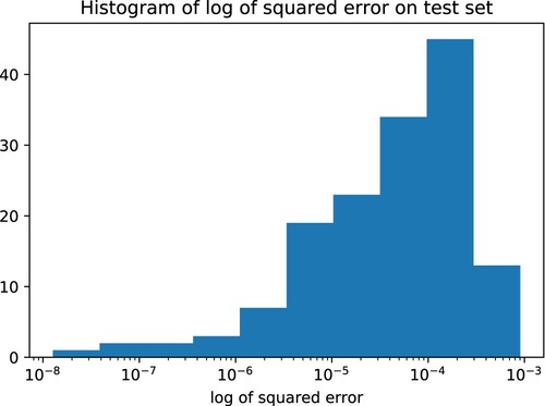
We stress the importance of point (iii) above by directing reader's attention to Figure 1, where we test generalization error of trained neural network for the five-dimensional family of PDEs corresponding to pricing a basket option under the Black–Scholes model. We refer reader to Example A.2 for details. We see that while the average error over test set is of order $\approx {10}^{-5}$, the errors for a given input vary significantly. Indeed, it has been observed in deep learning community that for high dimensional problems one can find input data such that trained neural network that appears to generalize well (i.e., achieves small errors on the out of training data) produces poor results (Goodfellow, Shlens, and Szegedy 2014).

Figure 1. Histogram of mean-square-error of solution to the PDE on the test data set.

1.2. Literature Review

Deep neural networks trained with stochastic gradient descent proved to be extremely successful in number of applications such as computer vision, natural language processing, generative models or reinforcement learning (LeCun, Bengio, and Hinton 2015). The application to PDE solvers is relatively new and has been pioneered by Weinan, Han, and Jentzen (2017), Han, Jentzen, and Weinan (2017) and Sirignano and Spiliopoulos (2017). See also Cvitanic and Zhang (2005) for the ideas of solving PDEs with gradient methods and for direct PDE approximation algorithm. PDEs provide an excellent test bed for neural networks approximation because (a) there exists alternative solvers, e.g., Monte Carlo, (b) we have well-developed theory for PDEs, and that knowledge can be used to tune algorithms. This is contrast to mainstream neural network approximations in text or images classification.

Apart from growing body of empirical results in the literature on ‘Deep PDEs solvers’, Chan-Wai-Nam, Mikael, and Warin (2019), Huré, Pham, and Warin (2019), Beck et al. (2018), Jacquier and Oumgari (2019) and Henry-Labordere (2017), there has been also some important theoretical contributions. It has been proved that deep artificial neural networks approximate solutions to parabolic PDEs to an arbitrary accuracy without suffering from the curse of dimensionality. The first mathematically rigorous proofs are given in Grohs et al. (2018) and Jentzen, Salimova, and Welti (2018). The high level idea is to show that neural network approximation to the PDE can be established by building on Feynman-Kac approximation and Monte Carlo approximation. By checking that Monte Carlo simulations do not suffer from the curse of dimensionality one can imply that the same is true for neural network approximation. Furthermore, it has been recently demonstrated in Hu et al. (2021) and Mei, Montanari, and Nguyen (2018) that noisy gradient descent algorithm used for training of neural networks of the form considered in Grohs et al. (2018) and Jentzen, Salimova, and Welti (2018) induces unique probability distribution function over the parameter space which minimizes learning. See Du et al. (2018), Chizat and Bach (2018), Rotskoff and Vanden-Eijnden (2018), Sirignano and Spiliopoulos (2020), Wang and Tang (2021) and Han and Long (2020) for related ideas on convergence of gradient algorithms for overparametrized neural networks. This means that there are theoretical guarantees for the approximation of (parabolic) PDEs with neural networks trained by noisy gradient methods alleviating the curse of dimensionality.

An important application of deep PDE solvers is that one can in fact approximate a parametric family of solutions of a PDE. To be more precise let $B\subseteq {\mathbb{R}}^p$, $p\ge 1$, be a parameter space. In the context of finance these, for example, might be initial volatility, volatility of volatility, interest rate and mean reversion parameters. One can approximate the parametric family of functions $F(\cdot ;\text{β}{)}_{\text{β}\in B}$ for an arbitrary range of parameters. This then allows for swift calibration of models to data (e.g. option prices). This is particularly appealing for high dimensional problems when calibrating directly using noisy Monte Carlo samples might be inefficient. This line of research gained some popularity recently and the idea has been tested numerically on various models and data sets (Horvath, Muguruza, and Tomas 2019; Liu et al. 2019; Bayer and Stemper 2018; Stone 2018; Hernandez 2016; Itkin 2019; McGhee 2018). There are some remarks that are in order. In the context of models calibration, while the training might be expensive one can do it offline, once and for good. One can also notice that training data could be used to produce a ‘look-up table’ taking model parameters to prices. From this perspective, the neural network, essentially, becomes an interpolator and a compression tool. Indeed the number of parameters of the network is much smaller than number of training data and therefore it is more efficient to store those. The final remark is that while there are other methods out there, such as Chebyshev functions, neural networks seem robust in high dimensions which make them our method of choice.

1.3. Notation

We denote by $\mathcal{D}\mathcal{N}$ the set of all fully connected feedforward neural networks (see Appendix 3). We also use $\mathcal{R}[f{]}_{\theta }\in \mathcal{D}\mathcal{N}$ with $\theta \in {\mathbb{R}}^{\kappa }$ to denote a neural network with weights θ approximating the function $f:{\mathbb{R}}^{d_0}\to {\mathbb{R}}^{d_1}$ for some $d_0,d_1\in \mathbb{N}$.

1.4. Outline

This paper is organized as follows. Section 2 provides theoretical underpinning for the derivation of all the algorithms we propose to solve (1(1) $\begin{array}{rl}& [{\mathrm{\partial }}_{t}v+b{\mathrm{\nabla }}_{x}v+\frac{1}{2}\mathrm{t}\mathrm{r}\left[{\mathrm{\nabla }}_x^{2}v{\sigma }^{\ast }\sigma \right]-cv](t,x;\text{β})=0,\\ & v(T,x;\text{β})=g(x;\text{β}),t\in [0,T],x\in {\mathbb{R}}^d,\text{β}\in B.\end{array}$(1) ). More specifically in Section 2.2 we combine the approximation of the gradient of the solution of the PDE resulting from the Deep Learning algorithms with Monte Carlo to obtain an unbiased approximation of the solution of the PDE. In Section 3, we describe the algorithms in detail.

Finally in Section 4, we provide numerical tests of the proposed algorithms. We empirically test these methods on relevant examples including a 100 dimensional option pricing problems, see Examples 4.4 and A.3. We carefully measure the training cost and report the variance reduction achieved.

Since we work in situation where the function approximated by neural network can be obtained via other methods ( Monte Carlo, PDE solution) we are able to test the how the expressiveness of fully connected artificial neural networks depends on the number of layers and neurons per layer. See Section A.2 for details.

2. PDE Martingale Control Variate

Control variate is one of the most powerful variance reduction techniques for Monte Carlo simulation. While a good control variate can reduce the computational cost of Monte Carlo computation by several orders of magnitude, it relies on judiciously chosen control variate functions that are problem specific. For example, when computing price of basket options a sound strategy is to choose control variates to be call options written on each of the stocks in the basket, since in many models these are priced by closed-form formulae. In this article, we are interested in black-box-type control variate approach by leveraging the Martingale Representation Theorem and neural networks. The idea of using Martingale Representation to obtain control variates goes back at least to Newton (1994). It has been further studied in combination with regression in Milstein and Tretyakov (2009) and Belomestny et al. (2018).

The bias in the approximation of the solution can be completely removed by employing control variates where the deep network provides the control variate resulting in very high variance reduction factor in the corresponding Monte Carlo simulation.

Let $(\mathrm{\Omega },\mathcal{F},\mathbb{P})$ be a probability space and consider an ${\mathbb{R}}^{d^{\prime }}$-valued Wiener process $W=(W^j{)}_{j=1}^{d^{\prime }}=((W_t^j{)}_{t\ge 0}{)}_{j=1}^{d^{\prime }}$. We will use $({\mathcal{F}}_t^W{)}_{t\ge 0}$ to denote the filtration generated by W. Consider a $D\subseteq {\mathbb{R}}^d$-valued, continuous, stochastic process defined for the parameters $\text{β}\in B\subseteq {\mathbb{R}}^p$, $X^{\text{β}}=(X^{\text{β},i}{)}_{i=1}^d=((X_t^{\text{β},i}{)}_{t\ge 0}{)}_{i=1}^d$ adapted to $({\mathcal{F}}_t^W{)}_{t\ge 0}$ given as the solution to (2) $\mathrm{d}{X}_s^{\text{β}}=b(s,X_s^{\text{β}};\text{β})\mathrm{d}s+\sigma (s,X_s;\text{β})\mathrm{d}{W}_s,s\in [t,T],X_t^{\text{β}}=x\in {\mathbb{R}}^d.$(2) We will use $({\mathcal{F}}_t^{\text{β}}{)}_{t\ge 0}$ to denote the filtration generated by $X^{\text{β}}$.

Let $g:{\mathbb{R}}^d\to \mathbb{R}$ be a measurable function and we assume that there is a (stochastic) discount factor given by $D(t_1,t_2;\text{β}):=e^{-{\int }_{t_1}^{t_2}c(s,X_s^{\text{β}};\text{β})\mathrm{d}s}$ for an appropriate function $c=c(t,x;\text{β})$. We will omit β from the discount factor notation for brevity. We now interpret $\mathbb{P}$ as some risk-neutral measure and so the $\mathbb{P}$-price of our contingent claim is (3) $v(t,x;\text{β}):=\mathbb{E}[D(t,T)g\left(X_T^{\text{β}}\right)|X_t^{\text{β}}=x].$(3) Say we have iid r.v.s $(X_T^{\text{β},i}{)}_{i=1}^N$ with the same distribution as $X_T^{\text{β}}$, where for each i, $X_t^{\text{β},i}=x$. Then the standard Monte Carlo estimator is $v^N(t,x;\text{β}):=\frac{1}{N}\sum _{i=1}^N{D}^i(t,T)g\left(X_T^{\text{β},i}\right).$ Convergence $v^N(t,x;\text{β})\to v(t,x;\text{β})$ in probability as $N\to \mathrm{\infty }$ is granted by the Law of Large Numbers. Moreover the classical Central Limit Theorem tells that $\mathbb{P}\left(v\right(t,x;\text{β})\in \left[v^N\right(t,x;\text{β})-z_{\alpha /2}\frac{\sigma }{\sqrt{N}},v^N(t,x;\text{β})+z_{\alpha /2}\frac{\sigma }{\sqrt{N}}])\to 1-\alpha \mathrm{a}\mathrm{s}N\to \mathrm{\infty },$ where $\sigma :=\sqrt{\mathbb{V}ar\left[D\right(t,T\left)g\right(X_T^{\text{β}}\left)\right]}$ and $z_{\alpha /2}$ is such that $1-\mathrm{\Phi }\left(z_{\alpha /2}\right)=\alpha /2$ with Φ being distribution function (cumulative distribution function) of the standard normal distribution. To decrease the width of the confidence intervals one can increase N, but this also increases the computational cost. A better strategy is to reduce variance by finding an alternative Monte Carlo estimator, say ${\mathcal{V}}^N(t,x;\text{β})$, such that (4) $\mathbb{E}\left[{\mathcal{V}}^N\right(t,x;\text{β}\left)\right]=v(t,x;\text{β})\mathrm{a}\mathrm{n}\mathrm{d}\mathbb{V}ar\left[{\mathcal{V}}^N\right(t,x;\text{β}\left)\right]<\mathbb{V}ar\left[v^N\right(t,x;\text{β}\left)\right],$(4) and the cost of computing ${\mathcal{V}}^N(t,x;\text{β})$ is similar to $v^N(t,x;\text{β})$.

In the remainder of the article, we will devise and test several strategies, based on deep learning, to find a suitable approximation for ${\mathcal{V}}^N(t,x;\text{β})$, by exploring the connection of the SDE (2(2) $\mathrm{d}{X}_s^{\text{β}}=b(s,X_s^{\text{β}};\text{β})\mathrm{d}s+\sigma (s,X_s;\text{β})\mathrm{d}{W}_s,s\in [t,T],X_t^{\text{β}}=x\in {\mathbb{R}}^d.$(2) ) and its associated PDE.

2.1. PDE Derivation of the Control Variate

It can be shown that under suitable assumptions on b, σ, c and g, and fixed $\text{β}\in B$ that $v\in C^{1,2}\left(\right[0,T]\times D)$. See, e.g.,  Krylov (1999). Let $a:=\frac{1}{2}\sigma {\sigma }^{\ast }$. Then, from Feynman–Kac formula (see, e.g., Th. 8.2.1 in  Øksendal 2003), we get (5) $\{\begin{array}{l}[{\mathrm{\partial }}_{t}v+\mathrm{t}\mathrm{r}(a{\mathrm{\partial }}_x^{2}v)+b{\mathrm{\partial }}_{x}v-cv](t,x;\text{β})=0\mathrm{i}\mathrm{n}[0,T)\times D,\\ v(T,\cdot )=g\mathrm{o}\mathrm{n}D.\end{array}$(5) Since $v\in C^{1,2}\left(\right[0,T]\times D)$ and since v satisfies the above PDE, if we apply Itô's formula then we obtain (6) $D(t,T)v(T,X_T^{\text{β}};\text{β})=v(t,x;\text{β})+{\int }_t^{T}D(t,s){\mathrm{\partial }}_{x}v(s,X_s^{\text{β}};\text{β})\sigma (s,X_s^{\text{β}};\text{β})\mathrm{d}{W}_s.$(6) Hence Feynman–Kac representation together with the fact that $v(T,X_T^{\text{β}};\text{β})=g\left(X_T^{\text{β}}\right)$ yields (7) $v(t,x;\text{β})=D(t,T)g\left(X_T^{\text{β}}\right)-{\int }_t^{T}D(t,s){\mathrm{\partial }}_{x}v(s,X_s^{\text{β}};\text{β})\sigma (s,X_s^{\text{β}};\text{β})\mathrm{d}{W}_s.$(7) Provided that $\underset{s\in [t,T]}{sup}\mathbb{E}\left[|D\right(t,s\left){\mathrm{\partial }}_{x}v\right(s,X_s^{\text{β}};\text{β}\left)\sigma \right(s,X_s^{\text{β}};\text{β}\left){|}^2\right]<\mathrm{\infty },$ then the stochastic integral is a martingale. Thus we can consider the Monte Carlo estimator. (8) ${\mathcal{V}}^N(t,x;\text{β}):=\frac{1}{N}\sum _{i=1}^N\left\{D^i\right(t,T\left)g\right(X_T^{\text{β},i})-{\int }_t^T{D}^i(t,s\left){\mathrm{\partial }}_{x}v\right(s,X_s^{\text{β},i};\text{β}\left)\sigma \right(s,X_s^{\text{β},i};\text{β}\left)\mathrm{d}{W}_s^i\right\}.$(8) To obtain a control variate, we thus need to approximate ${\mathrm{\partial }}_{x}v$. If one used classical approximation techniques to the PDE, such as finite difference or finite element methods, one would run into the curse of the dimensionality – the very reason one employs Monte Carlo simulations in the first place. Artificial neural networks have been shown to break the curse of dimensionality in specific situations (Grohs et al. 2018). To be more precise, authors in Berner, Grohs, and Jentzen (2020), Elbrächter et al. (2022), Jentzen, Salimova, and Welti (2018), Grohs, Jentzen, and Salimova (2019), Hutzenthaler et al. (2020), Grohs et al. (2018), Kutyniok et al. (2020), Gonon et al. (2021) and Reisinger and Zhang (2020) have shown that there always exist a deep feed forward neural network and some parameters such that the corresponding neural network can approximate the solution of a linear PDE arbitrarily well in a suitable norm under reasonable assumptions (terminal condition and coefficients can be approximated by neural networks). Moreover, the number of parameters grows only polynomially in dimension and so there is no curse of dimensionality. However, while the papers above construct the network they do not tell us how to find the ‘good’ parameters. In practice, the parameter search still relies on gradient descent-based minimization over a non-convex landscape. The application of the deep-network approximation to the solution of the PDE as a martingale control variate is an ideal compromise.

If there is no exact solution to the PDE (5(5) $\{\begin{array}{l}[{\mathrm{\partial }}_{t}v+\mathrm{t}\mathrm{r}(a{\mathrm{\partial }}_x^{2}v)+b{\mathrm{\partial }}_{x}v-cv](t,x;\text{β})=0\mathrm{i}\mathrm{n}[0,T)\times D,\\ v(T,\cdot )=g\mathrm{o}\mathrm{n}D.\end{array}$(5) ), as would be the case in any reasonable application, then we will approximate ${\mathrm{\partial }}_{x}v$ by $\mathcal{R}[{\mathrm{\partial }}_{x}v{]}_{\theta }\in \mathcal{D}\mathcal{N}$.

To obtain an implementable algorithm we discretize the integrals in ${\mathcal{V}}_t^{\text{β},N,v}$ and take a partition of $[0,T]$ denoted $\pi :=\{t=t_0<\cdots <t_{N_{\mathrm{s}\mathrm{t}\mathrm{e}\mathrm{p}\mathrm{s}}}=T\}$, and consider an approximation of (2(2) $\mathrm{d}{X}_s^{\text{β}}=b(s,X_s^{\text{β}};\text{β})\mathrm{d}s+\sigma (s,X_s;\text{β})\mathrm{d}{W}_s,s\in [t,T],X_t^{\text{β}}=x\in {\mathbb{R}}^d.$(2) ) by $(X_{t_k}^{\text{β},\pi }{)}_{t_k\in \pi }$. For simplicity we approximate all integrals arising by Riemann sums always taking the left-hand point when approximating the value of the integrand.

The implementable control variate Monte Carlo estimator is then the form (9) $\begin{array}{rl}& {\mathcal{V}}^{\pi ,\theta ,\lambda ,N}(t,x;\text{β}):=\frac{1}{N}\sum _{i=1}^N\left\{\right(D^{\pi }(t,T){)}^{i}g\left(X_T^{\text{β},\pi ,i}\right)\phantom{\sum _{k=1}^{N_{\mathrm{s}\mathrm{t}\mathrm{e}\mathrm{p}\mathrm{s}}-1}}\\ & -\lambda \sum _{k=1}^{N_{\mathrm{s}\mathrm{t}\mathrm{e}\mathrm{p}\mathrm{s}}-1}\left(D^{\pi }\right(t,t_k\left){)}^i\mathcal{R}\right[{\mathrm{\partial }}_{x}v{]}_{\theta }(t_k,X_{t_k}^{\text{β},\pi ,i};\text{β})\sigma (t_k,X_{t_k}^{\text{β},\pi ,i};\text{β})(W_{t_{k+1}}^i-W_{t_k}^i)\},\end{array}$(9) where $D^{\pi }(t,T):=e^{-\sum _{k=1}^{N_{\mathrm{s}\mathrm{t}\mathrm{e}\mathrm{p}\mathrm{s}}-1}c(t_k,X_{t_k}^{\text{β},\pi })(t_{k+1}-t_k)}$ and λ is a free parameter to be chosen (because we discretize and use approximation to the PDE it is expected $\lambda \ne 1$). Again, we point out that the only bias of the above estimator comes from the numerical scheme used to solve the forward and backward processes. Nevertheless, $\mathcal{R}[{\mathrm{\partial }}_{x}v{]}_{\theta }$ does not add any additional bias independently of the choice θ. We will discuss possible approximation strategies for approximating ${\mathrm{\partial }}_{x}v$ with $\mathcal{R}[{\mathrm{\partial }}_{x}v{]}_{\theta }$ in the following section.

In this section, we have actually derived an explicit form of the Martingale representation (see, e.g.,  Cohen and Elliott 2015, Th. 14.5.1) of $D(t,T)g\left(X_T^{\text{β}}\right)$ in terms of the solution of the PDE associated to the process $X^{\text{β}}$, which is given as the solution to (2(2) $\mathrm{d}{X}_s^{\text{β}}=b(s,X_s^{\text{β}};\text{β})\mathrm{d}s+\sigma (s,X_s;\text{β})\mathrm{d}{W}_s,s\in [t,T],X_t^{\text{β}}=x\in {\mathbb{R}}^d.$(2) ). In Appendix 1, we provide a more general framework to build a low-variance Monte Carlo estimator ${\mathcal{V}}_t^N$ for any (possibly non-Markovian) ${\mathcal{F}}^W$-adapted process $X^{\text{β}}$.

2.2. Unbiased Parametric PDE Approximation

After having trained the networks $\mathcal{R}[{\mathrm{\partial }}_{x}v{]}_{\theta }$ (using any of Algorithms 2–3 that we will introduce in Section 3) and $\mathcal{R}[v{]}_{\eta }$ (using any of Algorithms 2 and 3) that approximate $v,{\mathrm{\partial }}_{x}v$ one then has two options to approximate $v(t,x_t;\text{β})$

1. Directly with $\mathcal{R}\left[v{]}_{\eta }\right(t,x_t;\text{β})$ if Algorithms 2 or 3 were used, which will introduce some approximation bias.

2. By combining $\mathcal{R}[{\mathrm{\partial }}_{x}v{]}_{\theta }$ with the Monte Carlo approximation of $v(t,x_t;\text{β})$ using (9(9) $\begin{array}{rl}& {\mathcal{V}}^{\pi ,\theta ,\lambda ,N}(t,x;\text{β}):=\frac{1}{N}\sum _{i=1}^N\left\{\right(D^{\pi }(t,T){)}^{i}g\left(X_T^{\text{β},\pi ,i}\right)\phantom{\sum _{k=1}^{N_{\mathrm{s}\mathrm{t}\mathrm{e}\mathrm{p}\mathrm{s}}-1}}\\ & -\lambda \sum _{k=1}^{N_{\mathrm{s}\mathrm{t}\mathrm{e}\mathrm{p}\mathrm{s}}-1}\left(D^{\pi }\right(t,t_k\left){)}^i\mathcal{R}\right[{\mathrm{\partial }}_{x}v{]}_{\theta }(t_k,X_{t_k}^{\text{β},\pi ,i};\text{β})\sigma (t_k,X_{t_k}^{\text{β},\pi ,i};\text{β})(W_{t_{k+1}}^i-W_{t_k}^i)\},\end{array}$(9) ), which will yield an unbiased estimator of $v(t,x_t;\text{β})$. The complete method is stated as Algorithm 1.

3. Deep PDE Solvers

In this section, we propose two algorithms that learn the PDE solution (or its gradient) and then use it to build control variate using (9(9) $\begin{array}{rl}& {\mathcal{V}}^{\pi ,\theta ,\lambda ,N}(t,x;\text{β}):=\frac{1}{N}\sum _{i=1}^N\left\{\right(D^{\pi }(t,T){)}^{i}g\left(X_T^{\text{β},\pi ,i}\right)\phantom{\sum _{k=1}^{N_{\mathrm{s}\mathrm{t}\mathrm{e}\mathrm{p}\mathrm{s}}-1}}\\ & -\lambda \sum _{k=1}^{N_{\mathrm{s}\mathrm{t}\mathrm{e}\mathrm{p}\mathrm{s}}-1}\left(D^{\pi }\right(t,t_k\left){)}^i\mathcal{R}\right[{\mathrm{\partial }}_{x}v{]}_{\theta }(t_k,X_{t_k}^{\text{β},\pi ,i};\text{β})\sigma (t_k,X_{t_k}^{\text{β},\pi ,i};\text{β})(W_{t_{k+1}}^i-W_{t_k}^i)\},\end{array}$(9) ). We also include in Appendix 2 an additional algorithm to solve such linear PDEs using deep neural networks.

3.1. Projection Solver

Before we proceed further we recall a well-known property of conditional expectations, for proof see, e.g.,  Krylov (2002, Ch.3 Th. 14).

Theorem 3.1

Let $\mathcal{X}\in L^2\left(\mathcal{F}\right)$. Let $\mathcal{G}\subset \mathcal{F}$ be a sub σ-algebra. There exists a random variable $Y\in L^2\left(\mathcal{G}\right)$ such that $\mathbb{E}[|\mathcal{X}-\mathcal{Y}{|}^2]=\underset{\eta \in L^2\left(\mathcal{G}\right)}{inf}\mathbb{E}[|\mathcal{X}-\eta {|}^2].$ The minimizer, $\mathcal{Y}$, is unique and is given by $\mathcal{Y}=\mathbb{E}\left[\mathcal{X}|\mathcal{G}\right]$.

The theorem tell us that conditional expectation is an orthogonal projection of a random variable X onto $L^2\left(\mathcal{G}\right)$. Instead of working directly with (5(5) $\{\begin{array}{l}[{\mathrm{\partial }}_{t}v+\mathrm{t}\mathrm{r}(a{\mathrm{\partial }}_x^{2}v)+b{\mathrm{\partial }}_{x}v-cv](t,x;\text{β})=0\mathrm{i}\mathrm{n}[0,T)\times D,\\ v(T,\cdot )=g\mathrm{o}\mathrm{n}D.\end{array}$(5) ) we work with its probabilistic representation (6(6) $D(t,T)v(T,X_T^{\text{β}};\text{β})=v(t,x;\text{β})+{\int }_t^{T}D(t,s){\mathrm{\partial }}_{x}v(s,X_s^{\text{β}};\text{β})\sigma (s,X_s^{\text{β}};\text{β})\mathrm{d}{W}_s.$(6) ). To formulate the learning task, we replace $\mathcal{X}$ by $D(t,T)g\left(\right(X_T^{\text{β}}\left)\right)$ so that $v(t,X_t^{\text{β}};\text{β})=\mathbb{E}\left[\mathcal{X}|X_t^{\text{β}}\right]$. Hence, by Theorem (3.1), $\mathbb{E}[|\mathcal{X}-v(t,X_t^{\text{β}};\text{β}\left){|}^2\right]=\underset{\eta \in L^2\left(\sigma \right(X_t^{\text{β}}\left)\right)}{inf}\mathbb{E}[|\mathcal{X}-\eta {|}^2]$ and we know that for a fixed t the random variable which minimizes the mean square error is a function of $X_t$. But by the Doob–Dynkin Lemma (Cohen and Elliott 2015, Th. 1.3.12) we know that every $\eta \in L^2\left(\sigma \right(X_t\left)\right)$ can be expressed as $\eta =h_t\left(X_t^{\text{β}}\right)$ for some appropriate measurable $h_t$. For the practical algorithm, we restrict the search for the function $h_t$ to the class that can be expressed as deep neural networks $\mathcal{D}\mathcal{N}$. Hence we consider a family of functions ${\mathcal{R}}_{\theta }\in \mathcal{D}\mathcal{N}$ and set learning task as (10) ${\theta }^{\ast }:=\underset{\theta }{\mathrm{a}\mathrm{r}\mathrm{g}\mathrm{m}\mathrm{i}\mathrm{n}}{\mathbb{E}}_{\text{β}}\left[{\mathbb{E}}_{(X_t^{\text{β},\pi }{)}_{t\in \pi }}\left[\sum _{k=0}^{N_{\mathrm{s}\mathrm{t}\mathrm{e}\mathrm{p}\mathrm{s}}}{\left(D\right(t_k,T\left)g\right(X_T^{\text{β},\pi })-\mathcal{R}[v{]}_{{\theta }_{t_k}}(X_{t_k}^{\text{β},\pi };\text{β}))}^2\right]\right].$(10) The inner expectation in (10(10) ${\theta }^{\ast }:=\underset{\theta }{\mathrm{a}\mathrm{r}\mathrm{g}\mathrm{m}\mathrm{i}\mathrm{n}}{\mathbb{E}}_{\text{β}}\left[{\mathbb{E}}_{(X_t^{\text{β},\pi }{)}_{t\in \pi }}\left[\sum _{k=0}^{N_{\mathrm{s}\mathrm{t}\mathrm{e}\mathrm{p}\mathrm{s}}}{\left(D\right(t_k,T\left)g\right(X_T^{\text{β},\pi })-\mathcal{R}[v{]}_{{\theta }_{t_k}}(X_{t_k}^{\text{β},\pi };\text{β}))}^2\right]\right].$(10) ) is taken across all paths generated using numerical scheme on (2(2) $\mathrm{d}{X}_s^{\text{β}}=b(s,X_s^{\text{β}};\text{β})\mathrm{d}s+\sigma (s,X_s;\text{β})\mathrm{d}{W}_s,s\in [t,T],X_t^{\text{β}}=x\in {\mathbb{R}}^d.$(2) ) for a fixed β and it allows to solve the PDE (5(5) $\{\begin{array}{l}[{\mathrm{\partial }}_{t}v+\mathrm{t}\mathrm{r}(a{\mathrm{\partial }}_x^{2}v)+b{\mathrm{\partial }}_{x}v-cv](t,x;\text{β})=0\mathrm{i}\mathrm{n}[0,T)\times D,\\ v(T,\cdot )=g\mathrm{o}\mathrm{n}D.\end{array}$(5) ) for such β. The outer expectation is taken on β for which the distribution is fixed beforehand (e.g., uniform on B if it is compact), thus allowing the algorithm to find the optimal neural network weights ${\theta }^{\ast }$ to solve the parametric family of PDEs (5(5) $\{\begin{array}{l}[{\mathrm{\partial }}_{t}v+\mathrm{t}\mathrm{r}(a{\mathrm{\partial }}_x^{2}v)+b{\mathrm{\partial }}_{x}v-cv](t,x;\text{β})=0\mathrm{i}\mathrm{n}[0,T)\times D,\\ v(T,\cdot )=g\mathrm{o}\mathrm{n}D.\end{array}$(5) ). Automatic differentiation is used to approximate ${\mathrm{\partial }}_{x}v$. Algorithm 2 describes the method.

3.2. Probabilistic Representation Based on Backward SDE

Instead of working directly with (5(5) $\{\begin{array}{l}[{\mathrm{\partial }}_{t}v+\mathrm{t}\mathrm{r}(a{\mathrm{\partial }}_x^{2}v)+b{\mathrm{\partial }}_{x}v-cv](t,x;\text{β})=0\mathrm{i}\mathrm{n}[0,T)\times D,\\ v(T,\cdot )=g\mathrm{o}\mathrm{n}D.\end{array}$(5) ) we work with its probabilistic representation (6(6) $D(t,T)v(T,X_T^{\text{β}};\text{β})=v(t,x;\text{β})+{\int }_t^{T}D(t,s){\mathrm{\partial }}_{x}v(s,X_s^{\text{β}};\text{β})\sigma (s,X_s^{\text{β}};\text{β})\mathrm{d}{W}_s.$(6) ) and view it as a BSDE. To formulate the learning task based on this, we recall the time-grid π so that we can write it recursively as $\begin{array}{rl}& v(t_{N_{\mathrm{s}\mathrm{t}\mathrm{e}\mathrm{p}\mathrm{s}}},X_{t_{N_{\mathrm{s}\mathrm{t}\mathrm{e}\mathrm{p}\mathrm{s}}}}^{\text{β}};\text{β})=g\left(X_{t_{N_{\mathrm{s}\mathrm{t}\mathrm{e}\mathrm{p}\mathrm{s}}}}^{\text{β}}\right),\\ & D(t,t_{m+1})v(t_{m+1},X_{t_{m+1}}^{\text{β}};\text{β})=D(t,t_m)v(t_m,X_{t_m}^{\text{β}};\text{β})\\ & +{\int }_{t_m}^{t_{m+1}}D(t,s){\mathrm{\partial }}_{x}v(s,X_s^{\text{β}};\text{β})\sigma (s,X_s^{\text{β}};\text{β})\mathrm{d}{W}_s\mathrm{f}\mathrm{o}\mathrm{r}m=0,1,\dots ,N_{\mathrm{s}\mathrm{t}\mathrm{e}\mathrm{p}\mathrm{s}}-1.\end{array}$ Next consider deep network approximations for each time step in π and for both the solution of  (5(5) $\{\begin{array}{l}[{\mathrm{\partial }}_{t}v+\mathrm{t}\mathrm{r}(a{\mathrm{\partial }}_x^{2}v)+b{\mathrm{\partial }}_{x}v-cv](t,x;\text{β})=0\mathrm{i}\mathrm{n}[0,T)\times D,\\ v(T,\cdot )=g\mathrm{o}\mathrm{n}D.\end{array}$(5) ) and its gradient. $\mathcal{R}\left[v{]}_{{\eta }_m}\right(x;\text{β})\approx v(t_m,x;\text{β}),t_m\in \pi ,x\in {\mathbb{R}}^d$ and $\mathcal{R}\left[{\mathrm{\partial }}_{x}v{]}_{{\theta }_m}\right(x;\text{β})\approx {\mathrm{\partial }}_{x}v(t_m,x;\text{β}),t_m\in \pi ,x\in {\mathbb{R}}^d.$ Approximation depends on weights ${\eta }_m\in {\mathbb{R}}^{k_{\eta }}$, ${\theta }_m\in {\mathbb{R}}^{k_{\theta }}$. We then set the learning task as (11) $\begin{array}{rl}({\eta }^{\ast },{\theta }^{\ast })& :={\mathrm{a}\mathrm{r}\mathrm{g}\mathrm{m}\mathrm{i}\mathrm{n}}_{(\eta ,\theta )}{\mathbb{E}}_{\text{β},X^{\text{β}}}[{\left|g\right(X_{t_{N_{\mathrm{s}\mathrm{t}\mathrm{e}\mathrm{p}\mathrm{s}}}}^{\text{β},\pi })-\mathcal{R}[v{]}_{{\eta }_{N_{\mathrm{s}\mathrm{t}\mathrm{e}\mathrm{p}\mathrm{s}}}}\left(X_{t_{N_{\mathrm{s}\mathrm{t}\mathrm{e}\mathrm{p}\mathrm{s}}}}^{\text{β},\pi }\right)|}^2\phantom{\sum _{m=0}^{N_{\mathrm{s}\mathrm{t}\mathrm{e}\mathrm{p}\mathrm{s}}-1}}\\ & +\frac{1}{N_{\mathrm{s}\mathrm{t}\mathrm{e}\mathrm{p}\mathrm{s}}}\sum _{m=0}^{N_{\mathrm{s}\mathrm{t}\mathrm{e}\mathrm{p}\mathrm{s}}-1}|{\mathcal{E}}_{m+1}^{(\eta ,\theta )}{|}^2],\\ {\mathcal{E}}_{m+1}^{(\eta ,\theta )}& :=D(t,t_{m+1})\mathcal{R}\left[v{]}_{{\eta }_{m+1}}\right(X_{t_{m+1}}^{\text{β},\pi };\text{β})-D(t,t_m\left)\mathcal{R}\right[v{]}_{{\eta }_m}(X^{\text{β},\pi };\text{β})\\ & -D(t,t_m)\mathcal{R}\left[{\mathrm{\partial }}_{x}v{]}_{{\theta }_m}\right(X_{t_m}^{\text{β},\pi };\text{β}\left)\sigma \right(t_m,X_{t_m}^{\text{β},\pi };\text{β})\mathrm{\Delta }{W}_{t_{m+1}},\end{array}$(11) where $\eta =\{{\eta }_0,\dots ,{\eta }_{t_{N_{\mathrm{s}\mathrm{t}\mathrm{e}\mathrm{p}\mathrm{s}}}}\},\theta =\{{\theta }_0,\dots ,{\theta }_{t_{N_{\mathrm{s}\mathrm{t}\mathrm{e}\mathrm{p}\mathrm{s}}}}\}.$ The complete learning method is stated as Algorithm 3, where we split the optimization (11(11) $\begin{array}{rl}({\eta }^{\ast },{\theta }^{\ast })& :={\mathrm{a}\mathrm{r}\mathrm{g}\mathrm{m}\mathrm{i}\mathrm{n}}_{(\eta ,\theta )}{\mathbb{E}}_{\text{β},X^{\text{β}}}[{\left|g\right(X_{t_{N_{\mathrm{s}\mathrm{t}\mathrm{e}\mathrm{p}\mathrm{s}}}}^{\text{β},\pi })-\mathcal{R}[v{]}_{{\eta }_{N_{\mathrm{s}\mathrm{t}\mathrm{e}\mathrm{p}\mathrm{s}}}}\left(X_{t_{N_{\mathrm{s}\mathrm{t}\mathrm{e}\mathrm{p}\mathrm{s}}}}^{\text{β},\pi }\right)|}^2\phantom{\sum _{m=0}^{N_{\mathrm{s}\mathrm{t}\mathrm{e}\mathrm{p}\mathrm{s}}-1}}\\ & +\frac{1}{N_{\mathrm{s}\mathrm{t}\mathrm{e}\mathrm{p}\mathrm{s}}}\sum _{m=0}^{N_{\mathrm{s}\mathrm{t}\mathrm{e}\mathrm{p}\mathrm{s}}-1}|{\mathcal{E}}_{m+1}^{(\eta ,\theta )}{|}^2],\\ {\mathcal{E}}_{m+1}^{(\eta ,\theta )}& :=D(t,t_{m+1})\mathcal{R}\left[v{]}_{{\eta }_{m+1}}\right(X_{t_{m+1}}^{\text{β},\pi };\text{β})-D(t,t_m\left)\mathcal{R}\right[v{]}_{{\eta }_m}(X^{\text{β},\pi };\text{β})\\ & -D(t,t_m)\mathcal{R}\left[{\mathrm{\partial }}_{x}v{]}_{{\theta }_m}\right(X_{t_m}^{\text{β},\pi };\text{β}\left)\sigma \right(t_m,X_{t_m}^{\text{β},\pi };\text{β})\mathrm{\Delta }{W}_{t_{m+1}},\end{array}$(11) ) in several optimization problems, one per time step: learning the weights ${\theta }_m$ or ${\eta }_m$ at a certain time step $t_m<t_{N_{\mathrm{s}\mathrm{t}\mathrm{e}\mathrm{p}\mathrm{s}}}$ only requires knowing the weights ${\eta }_{m+1}$. At $m=N_{\mathrm{s}\mathrm{t}\mathrm{e}\mathrm{p}\mathrm{s}}$, learning the weights ${\eta }_{N_{\mathrm{s}\mathrm{t}\mathrm{e}\mathrm{p}\mathrm{s}}}$ only requires the terminal condition g. Note that the algorithm assumes that adjacent networks in time will be similar, and therefore we initialize ${\eta }_m$ and ${\theta }_m$ by ${\eta }_{m+1}^{\ast }$ and ${\theta }_{m+1}^{\ast }$.

3.3. Martingale Control Variate Deep Solvers

So far, the presented methodology to obtain the control variate consists on first learning the solution of the PDE and more importantly its gradient (Algorithms 2, 3) which is then plugged in (9(9) $\begin{array}{rl}& {\mathcal{V}}^{\pi ,\theta ,\lambda ,N}(t,x;\text{β}):=\frac{1}{N}\sum _{i=1}^N\left\{\right(D^{\pi }(t,T){)}^{i}g\left(X_T^{\text{β},\pi ,i}\right)\phantom{\sum _{k=1}^{N_{\mathrm{s}\mathrm{t}\mathrm{e}\mathrm{p}\mathrm{s}}-1}}\\ & -\lambda \sum _{k=1}^{N_{\mathrm{s}\mathrm{t}\mathrm{e}\mathrm{p}\mathrm{s}}-1}\left(D^{\pi }\right(t,t_k\left){)}^i\mathcal{R}\right[{\mathrm{\partial }}_{x}v{]}_{\theta }(t_k,X_{t_k}^{\text{β},\pi ,i};\text{β})\sigma (t_k,X_{t_k}^{\text{β},\pi ,i};\text{β})(W_{t_{k+1}}^i-W_{t_k}^i)\},\end{array}$(9) ). Alternatively, one can directly use the variance of (9(9) $\begin{array}{rl}& {\mathcal{V}}^{\pi ,\theta ,\lambda ,N}(t,x;\text{β}):=\frac{1}{N}\sum _{i=1}^N\left\{\right(D^{\pi }(t,T){)}^{i}g\left(X_T^{\text{β},\pi ,i}\right)\phantom{\sum _{k=1}^{N_{\mathrm{s}\mathrm{t}\mathrm{e}\mathrm{p}\mathrm{s}}-1}}\\ & -\lambda \sum _{k=1}^{N_{\mathrm{s}\mathrm{t}\mathrm{e}\mathrm{p}\mathrm{s}}-1}\left(D^{\pi }\right(t,t_k\left){)}^i\mathcal{R}\right[{\mathrm{\partial }}_{x}v{]}_{\theta }(t_k,X_{t_k}^{\text{β},\pi ,i};\text{β})\sigma (t_k,X_{t_k}^{\text{β},\pi ,i};\text{β})(W_{t_{k+1}}^i-W_{t_k}^i)\},\end{array}$(9) ) as the loss function to be optimized in order to learn the control variate. We expand this idea and design two additional algorithms.

Recall definition of ${\mathcal{V}}_{t,T}^{\text{β},\pi ,\theta ,\lambda ,N}$ given by (9(9) $\begin{array}{rl}& {\mathcal{V}}^{\pi ,\theta ,\lambda ,N}(t,x;\text{β}):=\frac{1}{N}\sum _{i=1}^N\left\{\right(D^{\pi }(t,T){)}^{i}g\left(X_T^{\text{β},\pi ,i}\right)\phantom{\sum _{k=1}^{N_{\mathrm{s}\mathrm{t}\mathrm{e}\mathrm{p}\mathrm{s}}-1}}\\ & -\lambda \sum _{k=1}^{N_{\mathrm{s}\mathrm{t}\mathrm{e}\mathrm{p}\mathrm{s}}-1}\left(D^{\pi }\right(t,t_k\left){)}^i\mathcal{R}\right[{\mathrm{\partial }}_{x}v{]}_{\theta }(t_k,X_{t_k}^{\text{β},\pi ,i};\text{β})\sigma (t_k,X_{t_k}^{\text{β},\pi ,i};\text{β})(W_{t_{k+1}}^i-W_{t_k}^i)\},\end{array}$(9) ). From (8(8) ${\mathcal{V}}^N(t,x;\text{β}):=\frac{1}{N}\sum _{i=1}^N\left\{D^i\right(t,T\left)g\right(X_T^{\text{β},i})-{\int }_t^T{D}^i(t,s\left){\mathrm{\partial }}_{x}v\right(s,X_s^{\text{β},i};\text{β}\left)\sigma \right(s,X_s^{\text{β},i};\text{β}\left)\mathrm{d}{W}_s^i\right\}.$(8) ) we know that the theoretical control variate Monte Carlo estimator has zero variance and so it is natural to set-up a learning task which aims to learn the network weights θ in a way which minimizes said variance: ${\theta }^{\star ,\mathrm{v}\mathrm{a}\mathrm{r}}:=\underset{\theta }{\mathrm{a}\mathrm{r}\mathrm{g}\mathrm{m}\mathrm{i}\mathrm{n}}\mathbb{V}\mathrm{a}\mathrm{r}[{\mathcal{V}}_{t,T}^{\text{β},\pi ,\theta ,\lambda ,N}].$ Setting $\lambda =1$, the learning task is stated as Algorithm 4.

We include a second similar Algorithm in Appendix 2.

4. Examples and Experiments

4.1. Options in Black–Scholes Model on d>1 Assets

Take a d-dimensional Wiener process W. We assume that we are given a symmetric, positive-definite matrix (covariance matrix) Σ and a lower triangular matrix C s.t. $\mathrm{\Sigma }=C{C}^{\ast }$. For such a positive-definite Σ we can always use Cholesky decomposition to find C. The risky assets will have volatilities given by ${\sigma }^i$. We will (abusing notation) write ${\sigma }^{ij}:={\sigma }^i{C}^{ij}$, when we don't need to separate the volatility of a single asset from correlations. The risky assets under the risk-neutral measure are then given by (12) $\mathrm{d}{S}_t^i=r{S}_t^i\mathrm{d}t+{\sigma }^i{S}_t^i\sum _j{C}^{ij}\mathrm{d}{W}_t^j.$(12) All sums will be from 1 to d unless indicated otherwise. Note that the SDE can be simulated exactly since $S_{t_{n+1}}^i=S_{t_n}^i\exp \left((r-\frac{1}{2}\sum _j({\sigma }^{ij}{)}^2)\right(t_{n+1}-t_n)+\sum _j{\sigma }^{ij}(W_{t_{n+1}}^j-W_{t_n}^j\left)\right).$ The associated PDE is (with $a^{ij}:=\sum _k{\sigma }^{ik}{\sigma }^{jk}$) ${\mathrm{\partial }}_{t}v(t,S)+\frac{1}{2}\sum _{i,j}{a}^{ij}{S}^i{S}^j{\mathrm{\partial }}_{x_i{x}_j}v(t,S)+r\sum _i{S}^i{\mathrm{\partial }}_{S^i}v(t,S)-rv(t,S)=0,$ for $(t,S)\in [0,T)\times ({\mathbb{R}}^{+}{)}^d$ together with the terminal condition $v(T,S)=g\left(S\right)$ for $S\in \mathbb{(}{\mathbb{R}}^{+}{)}^d$.

4.2. Deep Learning Setting

In this section, we describe the neural networks used in the four proposed algorithms as well as the training setting, in the specific situation where we have an options problem in Black–Scholes model on d>1 assets.

Learning Algorithms 3–5 share the same underlying fully connected artificial network which will be different for different $t_k$, $k=0,1,\dots ,N_{\mathrm{s}\mathrm{t}\mathrm{e}\mathrm{p}\mathrm{s}}-1$. At each time step, we use a fully connected artificial neural network denoted $\mathcal{R}[\cdot {]}_{{\theta }_k}\in \mathcal{D}\mathcal{N}$. The choice of the number of layers and network width is motivated by empirical results on different possible architectures applied on a short-lived options problem. We present the results of this study in Appendix A.2. The architecture is similar to that proposed in Beck et al. (2018).

At each time step, the network consists of four layers: one d-dimensional input layer, two $(d+20)$-dimensional hidden layers and one output layer. The output layer is one dimensional if the network is approximation for v and d-dimensional if the network is an approximation for ${\mathrm{\partial }}_{x}v$. The non-linear activation function used on the hidden layers is the linear rectifier relu. In all experiments except for Algorithm 3 for the basket options problem, we used batch normalization (Sergey Ioffe 2015) on the input of each network, just before the two nonlinear activation functions in front of the hidden layers and also after the last linear transformation.

The networks' optimal parameters are approximated by the Adam optimizer (Diederik and Kingma 2017) on the loss function specific for each method. Each parameter update (i.e. ,one step of the optimizer) is calculated on a batch of $5\cdot {10}^3$ paths $(x_{t_n}^i{)}_{n=0}^{N_{\mathrm{s}\mathrm{t}\mathrm{e}\mathrm{p}\mathrm{s}}}$ obtained by simulating the SDE. We take the necessary number of training steps until the stopping criteria defined below is met, with a learning rate of ${10}^{-3}$ during the first ${10}^4$ iterations, decreased to ${10}^{-4}$ afterwards.

During training of any of the algorithms, the loss value at each iteration is kept. A model is assumed to be trained if the difference between the loss averages of the two last consecutive windows of length 100 is less than a certain ϵ.

4.3. Evaluating Variance Reduction

We use the specified network architectures to assess the variance reduction in several examples below. After training the models in each particular example, they are evaluated as follows:

1. We calculate $N_{\mathrm{M}\mathrm{C}}=10$ times the Monte Carlo estimate $\overline{{\mathrm{\Xi }}_T}:=\frac{1}{N_{\mathrm{i}\mathrm{n}}}\sum _{i=1}^{N_{\mathrm{i}\mathrm{n}}}{\mathrm{\Xi }}_T^i$ and the Monte Carlo with control variate estimate ${\overline{\mathcal{V}}}_{t,T}^{\pi ,\theta ,\lambda ,N_{\mathrm{s}\mathrm{t}\mathrm{e}\mathrm{p}\mathrm{s}}}=\frac{1}{N_{\mathrm{i}\mathrm{n}}}\sum _{i=1}^{N_{\mathrm{i}\mathrm{n}}}{\mathcal{V}}_{t,T}^{\pi ,\theta ,\lambda ,N_{\mathrm{s}\mathrm{t}\mathrm{e}\mathrm{p}\mathrm{s}},i}$ using $N_{\mathrm{i}\mathrm{n}}={10}^6$ Monte Carlo samples.

2. From Central Limit Theorem, as $N_{\mathrm{i}\mathrm{n}}$ increases the standardized estimators converge in distribution to the Normal. Therefore, a 95% confidence interval of the variance of the estimator is given by $[\frac{(N_{\mathrm{M}\mathrm{C}}-1)S^2}{{\chi }_{1-\alpha /2,N_{\mathrm{M}\mathrm{C}}-1}},\frac{(N_{\mathrm{M}\mathrm{C}}-1)S^2}{{\chi }_{\alpha /2,N_{\mathrm{M}\mathrm{C}}-1}}]$ where S is the sample variance of the $N_{\mathrm{M}\mathrm{C}}$ controlled estimators ${\overline{\mathcal{V}}}_{t,T}^{\pi ,\theta ,\lambda ,N_{\mathrm{s}\mathrm{t}\mathrm{e}\mathrm{p}\mathrm{s}}}$, and $\alpha =0.05$. These are calculated for both the Monte Carlo estimate and the Monte Carlo with control variate estimate.

3. We use the $N_{\mathrm{M}\mathrm{C}}\cdot N_{\mathrm{i}\mathrm{n}}={10}^7$ generated samples ${\mathrm{\Xi }}_T^i$ and ${\mathcal{V}}_{t,T}^{\pi ,\theta ,\lambda ,N_{\mathrm{s}\mathrm{t}\mathrm{e}\mathrm{p}\mathrm{s}},i}$ to calculate and compare the empirical variances ${\tilde{\sigma }}_{{\mathrm{\Xi }}_T}^2$ and ${\tilde{\sigma }}_{{\mathcal{V}}_{t,T}^{\pi ,\theta ,\lambda ,N_{\mathrm{s}\mathrm{t}\mathrm{e}\mathrm{p}\mathrm{s}},i}}^2$.

4. The number of optimizer steps and equivalently number of random paths generated for training provide a cost measure of the proposed algorithms.

5. We evaluate the variance reduction if we use the trained models to create control variates for options in Black–Scholes models with different volatilities than the one used to train our models.

Example 4.1

Low dimensional problem with explicit solution

We consider exchange option on two assets. In this case, the exact price is given by the Margrabe formula. We take d = 2, $S_0^i=100$, $r=5\mathrm{\%}$, ${\sigma }^i=30\mathrm{\%}$, ${\mathrm{\Sigma }}^{ii}=1$, ${\mathrm{\Sigma }}^{ij}=0$ for $i\ne j$. The payoff is $g\left(S\right)=g(S^{\left(1\right)},S^{\left(2\right)}):=max(0,S^{\left(1\right)}-S^{\left(2\right)}).$ From Margrabe's formula, we know that $v(0,S)=\mathrm{B}\mathrm{l}\mathrm{a}\mathrm{c}\mathrm{k}\mathrm{S}\mathrm{c}\mathrm{h}\mathrm{o}\mathrm{l}\mathrm{e}\mathrm{s}(\mathrm{r}\mathrm{i}\mathrm{s}\mathrm{k}\mathrm{y}\mathrm{p}\mathrm{r}\mathrm{i}\mathrm{c}\mathrm{e}=\frac{S^{\left(1\right)}}{S^{\left(2\right)}},\mathrm{s}\mathrm{t}\mathrm{r}\mathrm{i}\mathrm{k}\mathrm{e}=1,T,r,\overline{\sigma }),$ where $\overline{\sigma }:=\sqrt{({\sigma }^{11}-{\sigma }^{21}{)}^2+({\sigma }^{22}-{\sigma }^{12}{)}^2}$.

We organize the experiment as follows: We train our models with batches of 5000 random paths $(s_{t_n}^i{)}_{n=0}^{N_{\mathrm{s}\mathrm{t}\mathrm{e}\mathrm{p}\mathrm{s}}}$ sampled from the SDE (12(12) $\mathrm{d}{S}_t^i=r{S}_t^i\mathrm{d}t+{\sigma }^i{S}_t^i\sum _j{C}^{ij}\mathrm{d}{W}_t^j.$(12) ), where $N_{\mathrm{s}\mathrm{t}\mathrm{e}\mathrm{p}\mathrm{s}}=50$. The assets' initial values $s_{t_0}^i$ are sampled from a lognormal distribution $X\sim \exp \left(\right(\mu -0.5{\sigma }^2)\tau +\sigma \sqrt{\tau }\xi ),$ where $\xi \sim \mathcal{N}(0,1),\mu =0.08,\tau =0.1$. The existence of an explicit solution allows to build a control variate of the form (9(9) $\begin{array}{rl}& {\mathcal{V}}^{\pi ,\theta ,\lambda ,N}(t,x;\text{β}):=\frac{1}{N}\sum _{i=1}^N\left\{\right(D^{\pi }(t,T){)}^{i}g\left(X_T^{\text{β},\pi ,i}\right)\phantom{\sum _{k=1}^{N_{\mathrm{s}\mathrm{t}\mathrm{e}\mathrm{p}\mathrm{s}}-1}}\\ & -\lambda \sum _{k=1}^{N_{\mathrm{s}\mathrm{t}\mathrm{e}\mathrm{p}\mathrm{s}}-1}\left(D^{\pi }\right(t,t_k\left){)}^i\mathcal{R}\right[{\mathrm{\partial }}_{x}v{]}_{\theta }(t_k,X_{t_k}^{\text{β},\pi ,i};\text{β})\sigma (t_k,X_{t_k}^{\text{β},\pi ,i};\text{β})(W_{t_{k+1}}^i-W_{t_k}^i)\},\end{array}$(9) ) using the known exact solution to obtain ${\mathrm{\partial }}_{x}v$. For a fixed number of time steps $N_{\mathrm{s}\mathrm{t}\mathrm{e}\mathrm{p}\mathrm{s}}$ this provides an upper bound on the variance reduction an artificial neural network approximation of ${\mathrm{\partial }}_{x}v$ can achieve.

We follow the evaluation framework to evaluate the model, simulating $N_{\mathrm{M}\mathrm{C}}\cdot N_{\mathrm{i}\mathrm{n}}$ paths by simulating (12(12) $\mathrm{d}{S}_t^i=r{S}_t^i\mathrm{d}t+{\sigma }^i{S}_t^i\sum _j{C}^{ij}\mathrm{d}{W}_t^j.$(12) ) with constant $(S_0^1,S_0^2{)}^i=(1,1)$. We report the following results:

1. Table 1 provides the empirical variances calculated over ${10}^6$ generated Monte Carlo samples and their corresponding control variates. The variance reduction measure indicates the quality of each control variate method. The variance reduction using the control variate given by Margrabe's formula provides a benchmark for our methods. Table 1 also provides the cost of training for each method, given by the number of optimizer iterations performed before hitting the stopping criteria, defined defined before with $ϵ=5\times {10}^{-6}$. We add an additional row with the control variate built using automatic differentiation on the network parametrized using the Deep Galerkin Method (Sirignano and Spiliopoulos 2017). The DGM attempts to find the optimal parameters of the network satisfying the PDE on a pre-determined time and space domain. In contrast to our algorithms, the DGM method is not restricted to learn the solution of the PDE on the paths built from the probabilistic representation of the PDE. However, this is what is precisely enhancing the performance of our methods in terms of variance reduction, since they are specifically learning an approximation to the solution of the PDE and its gradient such that the resulting control variate will yield a low-variance Monte Carlo estimator.

2. Table 2 provides the confidence intervals for the variances and of the Monte Carlo estimator, and the Monte Carlo estimator with control variate assuming these are calculated on ${10}^6$ random paths. Moreover, we add the confidence interval of the variance of the Monte Carlo estimator calculated over $N_{in}$ antithetic paths where the first $N_{in}/2$ Brownian paths generated using $(Z_i{)}_{i=1,\dots ,N_{steps}}$ samples from a normal and the second half of the Brownian paths are generated using the antithetic samples $(-Z_i{)}_{i=1,\dots ,N_{steps}}$. See Belomestny, Iosipoi, and Zhivotovskiy (2017, Section 4.2) for more details. All the proposed algorithms in this paper outperform the Monte Carlo estimator and the Monte Carlo estimator with antithetic paths; compared to the latter, our algorithms produce unbiased estimators with variances that 2 orders of magnitude less.

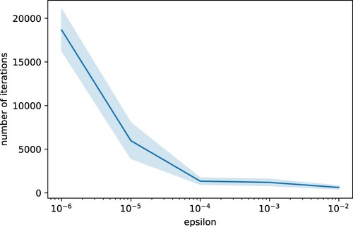
3. Figure 2 studies the iterative training for the BSDE solver. As it has been observed before, this type of training does not allow us to study the overall loss function as the number of training steps increases. Therefore we train the same model four times for different values of ϵ between 0.01 and $5\times {10}^{-6}$ and we study the number of iterations necessary to meet the stopping criteria defined by ϵ, the variance reduction once the stopping criteria is met, and the relationship between the number of iterations and the variance reduction. Note that the variance reduction stabilizes for $ϵ<{10}^{-5}$. Moreover, the number of iterations necessary to meet the stopping criteria increases exponentially as ϵ decreases, and therefore for our results printed in Tables 1 and 2 we employ $ϵ=5\times {10}^{-6}$ (Figure 3).

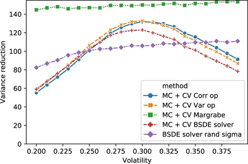
4. Figure 4 displays the variance reduction after using the trained models on several Black Scholes problem with exchange options but with values of σ other than 0.3 which was the one used for training. We see that the various algorithms work similarly well in this case (not taking training cost into account). We note that the variance reduction is close to the theoretical maximum which is restricted by time discretization. Finally we see that the variance reduction is still significant even when the neural network was trained with different model parameters (in our case volatility in the option pricing example). The labels of Figure 4 can be read as follows:

   1. MC + CV Corr op: Monte Carlo estimate with Deep Learning-based Control Variate built using Algorithm 5.

   2. MC + CV Var op: Monte Carlo estimate with Deep Learning-based Control Variate built using Algorithm 4.

   3. MC + CV BSDE solver: Monte Carlo estimate with Deep Learning-based Control Variate built using Algorithm 3.

   4. MC + CV Margrabe: Monte Carlo estimate with Control Variate using analytical solution for this problem given by Margrabe formula.

Figure 2. Left: Variance reduction in terms of number of optimizer iterations. Right: Variance reduction in terms of epsilon. Both are for Example 4.1 and Algorithm 3.

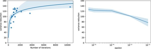
Figure 3. Number of optimizer iterations in terms of epsilon for Example 4.1 and Algorithm 3.

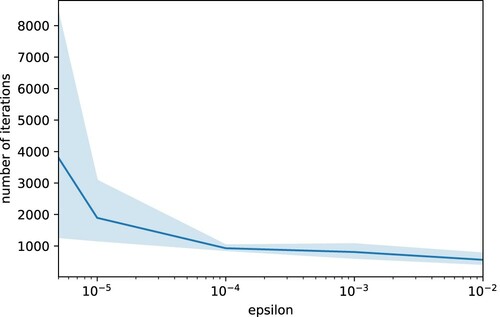
Figure 4. Variance reduction achieved by network trained with $\sigma =0.3$ but then applied in situations where $\sigma \in [0.2,0.4]$. We can see that the significant variance reduction is achieved by a neural network that was trained with ‘incorrect’ σ. Note that the ‘MC + CV Margbrabe’ displays the optimal variance reduction that can be achieved by using exact solution to the problem. The variance reduction is not infinite even in this case since stochastic integrals are approximated by Riemann sums.

Table 1. Results on exchange option problem on two assets, Example 4.1. Empirical Variance and variance reduction factor.

Method	Emp. var.	Var. red. fact.	Train. paths	Opt. steps
Monte Carlo	$3.16\times {10}^{-2}$	–	–	–
Algorithm 2	$2.47\times {10}^{-4}$	127.7	$38\times {10}^6$	$7600$
Algorithm 3	$2.59\times {10}^{-4}$	121.98	$6.945\times {10}^6$	1380
Algorithm 4	$2.39\times {10}^{-4}$	132.28	$36.055\times {10}^6$	7211
Algorithm 5	$2.40\times {10}^{-4}$	131.53	$45.61\times {10}^6$	9122
MC + CV Margrabe	$2.12\times {10}^{-4}$	149.19	–	–
MC + CV DGM (Sirignano and Spiliopoulos 2017)	$1.22\times {10}^{-3}$	25.8	–	–

Table 2. Results on exchange option problem on two assets, Example 4.1.

Method	Confidence interval variance	Confidence interval estimator
Monte Carlo	$[2.36\times {10}^{-6},4.15\times {10}^{-6}]$	$[0.1187,0.1195]$
Monte Carlo + antithetic paths	$[1.15\times {10}^{-6},2.02\times {10}^{-6}]$	$[0.1191,0.1195]$
Algorithm 2	$[4.13\times {10}^{-9},1.09\times {10}^{-8}]$	$[0.11919,0.11926]$
Algorithm 3	$[4.12\times {10}^{-9},1.09\times {10}^{-8}]$	$[0.11919,0.11925]$
Algorithm 4	$[4.32\times {10}^{-9},1.14\times {10}^{-8}]$	$[0.11919,0.11926]$
Algorithm 5	$[2.30\times {10}^{-9},6.12\times {10}^{-8}]$	$[0.11920,0.11924]$
MC + CV Margrabe	$[3.10\times {10}^{-9},8.23\times {10}^{-9}]$	$[0.11919,0.11925]$
MC + CV DGM (Sirignano and Spiliopoulos 2017)	$[3.10\times {10}^{-9},8.23\times {10}^{-9}]$	$[0.11919,0.11925]$

Example 4.2

Low-dimensional problem with explicit solution – Approximation of Price using PDE solver compared to Control Variate

We consider exchange options on two assets as in Example 4.1. We consider algorithm 3 that can be applied in two different ways:

1. It directly approximates the solution of the PDE (5(5) $\{\begin{array}{l}[{\mathrm{\partial }}_{t}v+\mathrm{t}\mathrm{r}(a{\mathrm{\partial }}_x^{2}v)+b{\mathrm{\partial }}_{x}v-cv](t,x;\text{β})=0\mathrm{i}\mathrm{n}[0,T)\times D,\\ v(T,\cdot )=g\mathrm{o}\mathrm{n}D.\end{array}$(5) ) and its gradient in every point.

2. We can use ${\mathrm{\partial }}_{x}v$ to build the control variate using probabilistic representation of the PDE  (6(6) $D(t,T)v(T,X_T^{\text{β}};\text{β})=v(t,x;\text{β})+{\int }_t^{T}D(t,s){\mathrm{\partial }}_{x}v(s,X_s^{\text{β}};\text{β})\sigma (s,X_s^{\text{β}};\text{β})\mathrm{d}{W}_s.$(6) ).

We compare both applications by calculating the expected error of the $L^2$-error of each of them with respect to the analytical solution given by Margrabe formula. From Margrabe's formula, we know that $v(0,S)=\mathrm{B}\mathrm{l}\mathrm{a}\mathrm{c}\mathrm{k}\mathrm{S}\mathrm{c}\mathrm{h}\mathrm{o}\mathrm{l}\mathrm{e}\mathrm{s}(\mathrm{r}\mathrm{i}\mathrm{s}\mathrm{k}\mathrm{y}\mathrm{p}\mathrm{r}\mathrm{i}\mathrm{c}\mathrm{e}=\frac{S^{\left(1\right)}}{S^{\left(2\right)}},\mathrm{s}\mathrm{t}\mathrm{r}\mathrm{i}\mathrm{k}\mathrm{e}=1,T,r,\overline{\sigma }).$ Let $\mathcal{R}\left[v{]}_{{\eta }_0}\right(x)\approx v(0,x)$ be the Deep Learning approximation of price at any point at initial time, calculated using Algorithm 3, and $\mathcal{R}\left[{\mathrm{\partial }}_{x}v{]}_{{\theta }_m}\right(x)\approx {\mathrm{\partial }}_{x}v(t_m,x)$ be the Deep Learning approximation of its gradient for every time step in the time discretization. The aim of this experiment is to show how even if Algorithm 3 numerically converges to a biased approximation of $v(0,x)$ (see Figure 5 left), it is still possible to use $\mathcal{R}\left[{\mathrm{\partial }}_{x}v{]}_{{\theta }_m}\right(x)$ to build an unbiased Monte-Carlo approximation of $v(0,x)$ with low variance.

Figure 5. Left: Loss of Algorithm 3 and squared error of $\mathcal{R}\left[v\right](t,x_0)$ in terms of training iterations. Right: Expected MSE of the two different approaches with respect to analytical solution in terms of number of Monte Carlo samples.

We organize the experiment as follows.

1. We calculate the expected value of the $L^2$-error of $\mathcal{R}{\eta }_0\left(x\right)$ where each component of $x\in {\mathbb{R}}^2$ is sampled from a lognormal distribution: $\mathbb{E}\left[|v\right(0,x)-\mathcal{R}[v{]}_{{\eta }_0}\left(x\right){|}^2]\approx \frac{1}{N}\sum _{i=1}^N|v(0,x^i)-\mathcal{R}[v{]}_{{\eta }_0}\left(x^i\right){|}^2$

2. We calculate the expected value of the $L^2$-error of the Monte Carlo estimator with control variate where each component of $x\in {\mathbb{R}}^2$ is sampled from a lognormal distribution: $\mathbb{E}\left[|v\right(0,x)-{\mathcal{V}}_{0,T}^{\pi ,\theta ,\lambda ,N_{MC},x}{|}^2]\approx \frac{1}{N}\sum _{i=1}^N|v(0,x^i)-{\mathcal{V}}_{0,T}^{\pi ,\theta ,\lambda ,N_{MC},x^i}{|}^2,$ where ${\mathcal{V}}_{0,T}^{\pi ,\theta ,\lambda ,N_{MC},x}$ is given by  (9(9) $\begin{array}{rl}& {\mathcal{V}}^{\pi ,\theta ,\lambda ,N}(t,x;\text{β}):=\frac{1}{N}\sum _{i=1}^N\left\{\right(D^{\pi }(t,T){)}^{i}g\left(X_T^{\text{β},\pi ,i}\right)\phantom{\sum _{k=1}^{N_{\mathrm{s}\mathrm{t}\mathrm{e}\mathrm{p}\mathrm{s}}-1}}\\ & -\lambda \sum _{k=1}^{N_{\mathrm{s}\mathrm{t}\mathrm{e}\mathrm{p}\mathrm{s}}-1}\left(D^{\pi }\right(t,t_k\left){)}^i\mathcal{R}\right[{\mathrm{\partial }}_{x}v{]}_{\theta }(t_k,X_{t_k}^{\text{β},\pi ,i};\text{β})\sigma (t_k,X_{t_k}^{\text{β},\pi ,i};\text{β})(W_{t_{k+1}}^i-W_{t_k}^i)\},\end{array}$(9) ), and is calculated for different values of Monte Carlo samples.

3. We calculate the expected value of the $L^2$-error of the Monte Carlo estimator without control variate where each component of $x\in {\mathbb{R}}^2$ is sampled from a lognormal distribution: $\mathbb{E}\left[|v\right(0,x)-{\mathrm{\Xi }}_{0,T}^{\pi ,\theta ,\lambda ,N_{MC},x}{|}^2]\approx \frac{1}{N}\sum _{i=1}^N|v(0,x^i)-{\mathrm{\Xi }}_{0,T}^{\pi ,\theta ,\lambda ,N_{MC},x^i}{|}^2,$ where ${\mathrm{\Xi }}_{0,T}^{\pi ,\theta ,\lambda ,N_{MC},x}:=\frac{1}{N_{MC}}\sum _{j=1}^{N_{MC}}D(t,T)g\left(X_T^i\right)$

Figure 5 provides one realization of the described experiment for different Monte Carlo iterations between 10 and 200. It shows how in this realization, 60 Monte Carlo iterations are enough to build a Monte Carlo estimator with control variate having lower bias than the solution provided by Algorithm 3.

Example 4.3

Low-dimensional problem with explicit solution. Training on random values for volatility

We consider exchange option on two assets. In this case, the exact price is given by the Margrabe formula. The difference with respect to the last example is that now we aim to generalize our model, so that it can build control variates for different Black–Scholes models. For this we take d = 2, $S_0^i=100$, r = 0.05, ${\sigma }^i\sim \mathrm{U}\mathrm{n}\mathrm{i}\mathrm{f}(0.2,0.4)$, ${\mathrm{\Sigma }}^{ii}=1$, ${\mathrm{\Sigma }}^{ij}=0$ for $i\ne j$.

The payoff is $g\left(S\right)=g(S^{\left(1\right)},S^{\left(2\right)}):=max(0,S^{\left(1\right)}-S^{\left(2\right)}).$ We organize the experiment as follows: for comparison purposes with the BSDE solver from the previous example, we train our model for exactly the same number of iterations, i.e. ,1380 batches of 5000 random paths $(s_{t_n}^i{)}_{n=0}^{N_{\mathrm{s}\mathrm{t}\mathrm{e}\mathrm{p}\mathrm{s}}}$ sampled from the SDE 12(12) $\mathrm{d}{S}_t^i=r{S}_t^i\mathrm{d}t+{\sigma }^i{S}_t^i\sum _j{C}^{ij}\mathrm{d}{W}_t^j.$(12) , where $N_{\mathrm{s}\mathrm{t}\mathrm{e}\mathrm{p}\mathrm{s}}=50$. The assets' initial values $s_{t_0}^i$ are sampled from a lognormal distribution $X\sim \exp \left(\right(\mu -0.5{\sigma }^2)\tau +\sigma \sqrt{\tau }\xi ),$ where $\xi \sim \mathcal{N}(0,1),\mu =0.08,\tau =0.1$. Since now σ can take different values, it is included as input to the networks at each time step.

The existence of an explicit solution allows to build a control variate of the form (9(9) $\begin{array}{rl}& {\mathcal{V}}^{\pi ,\theta ,\lambda ,N}(t,x;\text{β}):=\frac{1}{N}\sum _{i=1}^N\left\{\right(D^{\pi }(t,T){)}^{i}g\left(X_T^{\text{β},\pi ,i}\right)\phantom{\sum _{k=1}^{N_{\mathrm{s}\mathrm{t}\mathrm{e}\mathrm{p}\mathrm{s}}-1}}\\ & -\lambda \sum _{k=1}^{N_{\mathrm{s}\mathrm{t}\mathrm{e}\mathrm{p}\mathrm{s}}-1}\left(D^{\pi }\right(t,t_k\left){)}^i\mathcal{R}\right[{\mathrm{\partial }}_{x}v{]}_{\theta }(t_k,X_{t_k}^{\text{β},\pi ,i};\text{β})\sigma (t_k,X_{t_k}^{\text{β},\pi ,i};\text{β})(W_{t_{k+1}}^i-W_{t_k}^i)\},\end{array}$(9) ) using the known exact solution to obtain ${\mathrm{\partial }}_{x}v$. For a fixed number of time steps $N_{\mathrm{s}\mathrm{t}\mathrm{e}\mathrm{p}\mathrm{s}}$ this provides an upper bound on the variance reduction an artificial neural network approximation of ${\mathrm{\partial }}_{x}v$ can achieve.

Figure 6 adds the performance of this model to Figure 4, where the variance reduction of the Control Variate is displayed for different values of the volatility between 0.2 and 0.4.

Figure 6. Extension of Figure 4 with variance reduction achieved by training the model on different Black–Scholes models.

Example 4.4

High-dimensional problem, exchange against average

We extend the previous example to 100 dimensions. This example is similar to ${\mathrm{E}\mathrm{X}}_{10E}$ from Broadie, Du, and Moallemi (2015). We will take $S_0^i=100$, $r=5\mathrm{\%}$, ${\sigma }^i=30\mathrm{\%}$, ${\mathrm{\Sigma }}^{ii}=1$, ${\mathrm{\Sigma }}^{ij}=0$ for $i\ne j$.

We will take this to be $g\left(S\right):=max(0,S^1-\frac{1}{d-1}\sum _{i=2}^d{S}^i).$ The experiment is organized as follows: we train our models with batches of $5\cdot {10}^3$ random paths $(s_{t_n}^i{)}_{n=0}^{N_{\mathrm{s}\mathrm{t}\mathrm{e}\mathrm{p}\mathrm{s}}}$ sampled from the SDE (12(12) $\mathrm{d}{S}_t^i=r{S}_t^i\mathrm{d}t+{\sigma }^i{S}_t^i\sum _j{C}^{ij}\mathrm{d}{W}_t^j.$(12) ), where $N_{\mathrm{s}\mathrm{t}\mathrm{e}\mathrm{p}\mathrm{s}}=50$. The assets' initial values $s_{t_0}^i$ are sampled from a lognormal distribution $X\sim \exp \left(\right(\mu -0.5{\sigma }^2)\tau +\sigma \sqrt{\tau }\xi ),$ where $\xi \sim N(0,1)$, $\mu =0.08$, $\tau =0.1$.

We follow the evaluation framework to evaluate the model, simulating $N_{\mathrm{M}\mathrm{C}}\cdot N_{\mathrm{i}\mathrm{n}}$ paths by simulating (12(12) $\mathrm{d}{S}_t^i=r{S}_t^i\mathrm{d}t+{\sigma }^i{S}_t^i\sum _j{C}^{ij}\mathrm{d}{W}_t^j.$(12) ) with constant $S_0^i=1$ for $i=1,\dots ,100$. We have the following results:

1. Table 3 provides the empirical variances calculated over ${10}^6$ generated Monte Carlo samples and their corresponding control variates. The variance reduction measure indicates the quality of each control variate method. Table 3 also provides the cost of training for each method, given by the number of optimizer iterations performed before hitting the stopping criteria with $ϵ=5\cdot {10}^{-6}$. Algorithm 3 outperforms the other algorithms in terms of variance reduction factor. This is not surprising as Algorithm 3 explicitly learns the discretization of the Martingale representation (Equation (7(7) $v(t,x;\text{β})=D(t,T)g\left(X_T^{\text{β}}\right)-{\int }_t^{T}D(t,s){\mathrm{\partial }}_{x}v(s,X_s^{\text{β}};\text{β})\sigma (s,X_s^{\text{β}};\text{β})\mathrm{d}{W}_s.$(7) )) from which the control variate arises.

2. Table 4 provides the confidence interval for the variance of the Monte Carlo estimator, and the Monte Carlo estimator with control variate assuming these are calculated on ${10}^6$ random paths.

3. Figures 7 and 8 study the iterative training for the BSDE solver. We train the same model four times for different values of ϵ between 0.01 and $5\times {10}^{-6}$ and we study the number of iterations necessary to meet the stopping criteria defined by ϵ, the variance reduction once the stopping criteria is met, and the relationship between the number of iterations and the variance reduction. Note that in this case the variance reduction does not stabilize for $ϵ<{10}^{-5}$. However, the number of training iterations increases exponentially as ϵ decreases, and therefore we also choose $ϵ=5\times {10}^{-6}$ to avoid building a control that requires a high number of random paths to be trained (Figure 9).

Figure 7. Left: Variance reduction in terms of number of optimizer iterations. Right: Variance reduction in terms of epsilon. Both for Example 4.4 and Algorithm 3.

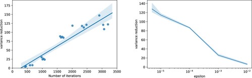
Figure 8. Number of optimizer iterations in terms of ϵ for Example 4.4 and Algorithm 3.

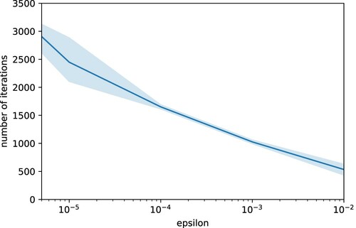
Figure 9. Variance reduction with network trained with $\sigma =0.3$ but applied for $\sigma \in [0.2,0.4]$ for the model of Example 4.4. We see that the variance reduction factor is considerable even in the case when the network is used with ‘wrong’ σ. It seems that Algorithm 4 is not performing well in this case.

Table 3. Results on exchange option problem on 100 assets, Example 4.4. Empirical Variance and variance reduction factor and costs in terms of paths used for training and optimizer steps.

Method	Emp. Var.	Var. Red. Fact.	Train. Paths	Opt. Steps
Monte Carlo	$1.97\times {10}^{-2}$	–	–	–
Algorithm 2	$5.94\times {10}^{-3}$	33.16	$74\times {10}^6$	$14900$
Algorithm 3	$1.51\times {10}^{-4}$	130.39	$14.145\times {10}^6$	$2829$
Algorithm 4	$5.29\times {10}^{-4}$	37.22	$97.265\times {10}^6$	$19453$
Algorithm 5	$1.93\times {10}^{-4}$	102.05	$76.03\times {10}^6$	$15206$

Table 4. Results on exchange option problem on 100 assets, Example 4.4.

Method	Confidence interval variance	Confidence interval estimator
Monte Carlo	$[1.51\times {10}^{-6},2.65\times {10}^{-6}]$	$[0.0845,0.0849]$
Monte Carlo + antithetic paths	$[8.77\times {10}^{-7},1.53\times {10}^{-6}]$	$[0.0845,0.0848]$
Algorithm 2	$[3.04\times {10}^{-8},2.14\times {10}^{-7}]$	$[0.0848,0.08493]$
Algorithm 3	$[5.32\times {10}^{-9},1.41\times {10}^{-8}]$	$[0.08485,0.8492]$
Algorithm 4	$[4.13\times {10}^{-9},1.09\times {10}^{-8}]$	$[0.08484,0.08490]$
Algorithm 5	$[3.80\times {10}^{-9},1.0\times {10}^{-8}]$	$[0.08487,0.08493]$

Disclosure statement

No potential conflict of interest was reported by the authors.

Additional information

Funding

This work was supported by the Alan Turing Institute under EPSRC grant no. EP/N510129/1.

Appendices

Appendix 1.

Martingale Control Variate

Let $(\mathrm{\Omega },\mathcal{F},\mathbb{P})$ be a probability space and consider an ${\mathbb{R}}^{d^{\prime }}$-valued Wiener process $W=(W^j{)}_{j=1}^{d^{\prime }}=((W_t^j{)}_{t\ge 0}{)}_{j=1}^{d^{\prime }}$. We will use $({\mathcal{F}}_t^W{)}_{t\ge 0}$ to denote the filtration generated by W. Consider a $D\subseteq {\mathbb{R}}^d$-valued, continuous, stochastic process defined for the parameters $\text{β}\in B\subseteq {\mathbb{R}}^p$, $X^{\text{β}}=(X^{\text{β},i}{)}_{i=1}^d=((X_t^{\text{β},i}{)}_{t\ge 0}{)}_{i=1}^d$ adapted to $({\mathcal{F}}_t^W{)}_{t\ge 0}$.

Let $g:C\left(\right[0,T],{\mathbb{R}}^d)\to \mathbb{R}$ be a measurable function. We shall consider path-dependent contingent claims of the form $g\left(\right(X_s^{\text{β}}{)}_{s\in [0,T]})$. Finally we assume that there is a (stochastic) discount factor given by $D(t_1,t_2;\text{β})=e^{-{\int }_{t_1}^{t_2}c(s,X_s^{\text{β}};\text{β})\mathrm{d}s}$ for an appropriate function $c=c(t,x;\text{β})$. We will omit the β from the discount factor notation. Let ${\mathrm{\Xi }}_T^{\text{β}}:=D(t,T)g\left(\right(X_s^{\text{β}}{)}_{s\in [0,T]}).$ We now interpret $\mathbb{P}$ as some risk-neutral measure and so the $\mathbb{P}$-price of our contingent claim is $V_t^{\text{β}}=\mathbb{E}\left[{\mathrm{\Xi }}_T^{\text{β}}|{\mathcal{F}}_t^{\text{β}}\right]=\mathbb{E}\left[D\right(t,T\left)g\right(\left(X_s^{\text{β}}{)}_{s\in [0,T]}\right)|{\mathcal{F}}_t^{\text{β}}].$ By assumption ${\mathrm{\Xi }}_T^{\text{β}}$ is ${\mathcal{F}}_T^W$ measurable and $\mathbb{E}\left[|{\mathrm{\Xi }}_T^{\text{β}}{|}^2\right]<\mathrm{\infty }$. Hence, from the Martingale Representation Theorem, see, e.g.,  Cohen and Elliott (2015, Th. 14.5.1), there exists a unique process $(Z_t^{\text{β}}{)}_t$ adapted to $({\mathcal{F}}_t^W{)}_t$ with $\mathbb{E}\left[{\int }_0^T|Z_s^{\text{β}}{|}^{2}ds\right]<\mathrm{\infty }$ such that (A1) ${\mathrm{\Xi }}_T^{\text{β}}=\mathbb{E}\left[{\mathrm{\Xi }}_T^{\text{β}}|{\mathcal{F}}_0^W\right]+{\int }_0^T{Z}_s^{\text{β}}\mathrm{d}{W}_s.$(A1) The proof of the existence of the process $(Z_t^{\text{β}}{)}_t$, is non-constructive. In the setup of the paper, we used the Markovian property of ${\mathrm{\Xi }}_t^{\text{β}}$ to approximate $Z_t^{\text{β}}$ via the associated linear PDE. In the more general non-Markovian setup, Cont and Lu (2016) provide a numerical method to construct the martingale representation.

Observe that in our setup, ${\mathcal{F}}_0={\mathcal{F}}_0^W$, ${\mathcal{F}}_t^{\text{β}}\subseteq {\mathcal{F}}_t^W$ for $t\ge 0$. Hence tower property of the conditional expectation implies that (A2) $\mathbb{E}\left[{\mathrm{\Xi }}_T^{\text{β}}|{\mathcal{F}}_t^{\text{β}}\right]=\mathbb{E}\left[{\mathrm{\Xi }}_T^{\text{β}}|{\mathcal{F}}_0^W\right]+{\int }_0^t{Z}_s^{\text{β}}\mathrm{d}{W}_s.$(A2) Consequently (A1(A1) ${\mathrm{\Xi }}_T^{\text{β}}=\mathbb{E}\left[{\mathrm{\Xi }}_T^{\text{β}}|{\mathcal{F}}_0^W\right]+{\int }_0^T{Z}_s^{\text{β}}\mathrm{d}{W}_s.$(A1) ) and (A2(A2) $\mathbb{E}\left[{\mathrm{\Xi }}_T^{\text{β}}|{\mathcal{F}}_t^{\text{β}}\right]=\mathbb{E}\left[{\mathrm{\Xi }}_T^{\text{β}}|{\mathcal{F}}_0^W\right]+{\int }_0^t{Z}_s^{\text{β}}\mathrm{d}{W}_s.$(A2) ) imply $\mathbb{E}\left[{\mathrm{\Xi }}_T^{\text{β}}|{\mathcal{F}}_t^{\text{β}}\right]={\mathrm{\Xi }}_T^{\text{β}}-{\int }_t^T{Z}_s^{\text{β}}\mathrm{d}{W}_s.$ We then observe that $V_t^{\text{β}}=\mathbb{E}\left[{\mathrm{\Xi }}_T^{\text{β}}|{\mathcal{F}}_t^{\text{β}}\right]=\mathbb{E}\left[{\mathrm{\Xi }}_T^{\text{β}}-{\int }_t^T{Z}_s^{\text{β}}\mathrm{d}{W}_s|{\mathcal{F}}_t^{\text{β}}\right].$ If we can generate iid $(W^i{)}_{i=1}^N$ and $(Z^{\text{β},i}{)}_{i=1}^N$ with the same distributions as W and Z respectively then we can consider the following Monte-Carlo estimator of $V_t^{\text{β}}$: ${\mathcal{V}}_t^{\text{β},N}:=\frac{1}{N}\sum _{i=1}^N({\mathrm{\Xi }}_T^{\text{β},i}-{\int }_t^T{Z}_s^{\text{β},i}\mathrm{d}{W}_s^i).$ In the companion paper (Sabate-Vidales, Šiška, and Szpruch 2020), we provide deep learning algorithms to price path-dependent options in the risk neutral measure by solving the corresponding path-dependent PDE, using a combination of Recurrent Neural networks and path signatures to parametrize the process $Z^{\text{β}}$.

Appendix 2.

Martingale Control Variate Deep Solvers

A.1. Empirical Correlation Maximization

This method is based on the idea that since we are looking for a good control variate we should directly train the network to maximize the variance reduction between the vanilla Monte-Carlo estimator and the control variates Monte-Carlo estimator by also trying to optimize λ.

Recall we denote ${\mathrm{\Xi }}_T=D(t,T)g\left(\right(X_s{)}_{s\in [t,T]})$. We also denote as $M_{t,T}$ as the stochastic integral that arises in the martingale representation of ${\mathrm{\Xi }}_T$. The optimal coefficient ${\lambda }^{\ast ,\theta }$ that minimizes the variance $\mathbb{V}\mathrm{a}\mathrm{r}[{\mathrm{\Xi }}_T-\lambda M_{t,T}^{\theta }]$ is ${\lambda }^{\ast ,\theta }=\frac{\mathbb{C}\mathrm{o}\mathrm{v}[{\mathrm{\Xi }}_T,M_{t,T}^{\theta }]}{\mathbb{V}\mathrm{a}\mathrm{r}\left[M_{t,T}^{\theta }\right]}.$ Let ${\rho }^{{\mathrm{\Xi }}_T,M_{t,T}^{\theta }}$ denote the Pearson correlation coefficient between ${\mathrm{\Xi }}_T$ and $M_{t,T}^{\theta }$, i.e., ${\rho }^{{\mathrm{\Xi }}_T,M_{t,T}^{\theta }}=\frac{\mathbb{C}\mathrm{o}\mathrm{v}({\mathrm{\Xi }}_T,M_{t,T}^{\theta })}{\sqrt{\mathbb{V}\mathrm{a}\mathrm{r}\left[{\mathrm{\Xi }}_T\right]\mathbb{V}\mathrm{a}\mathrm{r}\left[M_{t,T}^{\theta }\right]}}.$ With the optimal ${\lambda }^{\ast }$ we then have that the variance reduction obtained from the control variate is $\frac{\mathbb{V}\mathrm{a}\mathrm{r}\left[{\mathcal{V}}_{t,T}^{\pi ,\theta ,{\lambda }^{\ast },N}\right]}{\mathbb{V}\mathrm{a}\mathrm{r}\left[{\mathrm{\Xi }}_T\right]}=1-{\left({\rho }^{{\mathrm{\Xi }}_T,M_{t,T}^{\theta }}\right)}^2.$ See Glasserman (2013, Ch. 4.1) for more details. Therefore we set the learning task as ${\theta }^{\ast ,cor}:={\mathrm{a}\mathrm{r}\mathrm{g}\mathrm{m}\mathrm{i}\mathrm{n}}_{\theta }[1-{\left({\rho }^{{\mathrm{\Xi }}_T,M_{t,T}^{\theta }}\right)}^2].$ The implementable version requires the definition of ${\mathcal{V}}_{t,T}^{\text{β},\pi ,\theta ,\lambda ,N}$ in (9(9) $\begin{array}{rl}& {\mathcal{V}}^{\pi ,\theta ,\lambda ,N}(t,x;\text{β}):=\frac{1}{N}\sum _{i=1}^N\left\{\right(D^{\pi }(t,T){)}^{i}g\left(X_T^{\text{β},\pi ,i}\right)\phantom{\sum _{k=1}^{N_{\mathrm{s}\mathrm{t}\mathrm{e}\mathrm{p}\mathrm{s}}-1}}\\ & -\lambda \sum _{k=1}^{N_{\mathrm{s}\mathrm{t}\mathrm{e}\mathrm{p}\mathrm{s}}-1}\left(D^{\pi }\right(t,t_k\left){)}^i\mathcal{R}\right[{\mathrm{\partial }}_{x}v{]}_{\theta }(t_k,X_{t_k}^{\text{β},\pi ,i};\text{β})\sigma (t_k,X_{t_k}^{\text{β},\pi ,i};\text{β})(W_{t_{k+1}}^i-W_{t_k}^i)\},\end{array}$(9) ), where we set $\begin{array}{rl}{\mathrm{\Xi }}_T^{\text{β},\pi ,i}& :=D^{\pi }(t,T){)}^{i}g\left(X_T^{\text{β},\pi ,i}\right)\\ M_{t,T}^{\text{β},\pi ,i,\theta }& :=\sum _{k=1}^{N_{\mathrm{s}\mathrm{t}\mathrm{e}\mathrm{p}\mathrm{s}}-1}\left(D^{\pi }\right(t,t_k\left){)}^i\mathcal{R}\right[{\mathrm{\partial }}_{x}v{]}_{\theta }(t_k,X_{t_k}^{\text{β},\pi ,i})\sigma (t_k,X_{t_k}^{\text{β},\pi ,i})(W_{t_{k+1}}^i-W_{t_k}^i)\end{array}$ The full method is stated as Algorithm 5.

Appendix 3.

Artificial Neural Networks

We fix a locally Lipschitz function $\mathbf{a}:\mathbb{R}\to \mathbb{R}$ and for $d\in \mathbb{N}$ define ${\mathbf{A}}_d:{\mathbb{R}}^d\to {\mathbb{R}}^d$ as the function given, for $x=(x_1,\dots ,x_d)$ by ${\mathbf{A}}_d\left(x\right)=\left(\mathbf{a}\right(x_1),\dots ,\mathbf{a}(x_d\left)\right)$. We fix $L\in \mathbb{N}$ (the number of layers), $l_k\in \mathbb{N}$, $k=0,1,\dots L-1$ (the size of input to layer k) and $l_L\in \mathbb{N}$ (the size of the network output). A fully connected artificial neural network is then given by $\mathrm{\Phi }=\left(\right(W_1,B_1),\dots ,(W_L,B_L\left)\right)$, where, for $k=1,\dots ,L$, we have real $l_{k-1}\times l_k$ matrices $W_k$ and real $l_k$ dimensional vectors $B_k$.

The artificial neural network defines a function ${\mathcal{R}}_{\mathrm{\Phi }}:{\mathbb{R}}^{l_0}\to {\mathbb{R}}^{l_L}$ given recursively, for $x_0\in {\mathbb{R}}^{l_0}$, by ${\mathcal{R}}_{\mathrm{\Phi }}\left(x_0\right)=W_L{x}_{L-1}+B_L,x_k={\mathbf{A}}_{l_k}(W_k{x}_{k-1}+B_k),k=1,\dots ,L-1.$ We can also define the function $\mathcal{P}$ which counts the number of parameters as $\mathcal{P}\left(\mathrm{\Phi }\right)=\sum _{i=1}^L(l_{k-1}{l}_k+l_k).$ We will call such class of fully connected artificial neural networks $\mathcal{D}\mathcal{N}$. Note that since the activation functions and architecture are fixed the learning task entails finding the optimal $\mathrm{\Phi }\in {\mathbb{R}}^{\mathcal{P}\left(\mathrm{\Phi }\right)}$.

Appendix 4.

Additional Numerical Results

Example A.1

Low dimensional basket option

We consider the basket options problem of pricing, using the example from Belomestny, Iosipoi, and Zhivotovskiy (2017, Sec 4.2.3). The payoff function is $g\left(S\right):=max(0,\sum _{i=1}^d{S}^i-K).$ We first consider the basket options problem on two assets, with d = 2, $S_0^i=70$, $r=50\mathrm{\%}$, ${\sigma }^i=100\mathrm{\%}$, ${\mathrm{\Sigma }}^{ii}=1$, ${\mathrm{\Sigma }}^{ij}=0$ for $i\ne j$, and constant strike $K=\sum _{i=1}^d{S}_0^i$. In line with the example from Belomestny, Iosipoi, and Zhivotovskiy (2017, Sec 4.2.3) for comparison purposes we organize the experiment as follows. The control variates on 20, 000 batches of 5000 samples each of $(s_{t_n}^i{)}_{n=0}^{N_{\mathrm{s}\mathrm{t}\mathrm{e}\mathrm{p}\mathrm{s}}}$ by simulating the SDE 12(12) $\mathrm{d}{S}_t^i=r{S}_t^i\mathrm{d}t+{\sigma }^i{S}_t^i\sum _j{C}^{ij}\mathrm{d}{W}_t^j.$(12) , where $N_{\mathrm{s}\mathrm{t}\mathrm{e}\mathrm{p}\mathrm{s}}=50$. The assets' initial values $s_{t_0}$ are always constant $S_{t_0}^i=0.7$. We follow the evaluation framework to evaluate the model, simulating $N_{\mathrm{M}\mathrm{C}}\cdot N_{\mathrm{i}\mathrm{n}}$ paths by simulating 12(12) $\mathrm{d}{S}_t^i=r{S}_t^i\mathrm{d}t+{\sigma }^i{S}_t^i\sum _j{C}^{ij}\mathrm{d}{W}_t^j.$(12) with constant $S_0^i=0.7$ for $i=1,\dots ,100$. We have the following results:

1. Table A1 provides the empirical variances calculated over ${10}^6$ generated Monte Carlo samples and their corresponding control variates. The variance reduction measure indicates the quality of each control variate method. Table A1 also provides the cost of training for each method, given by the number of optimizer iterations performed before hitting the stopping criteria, defined defined before with $ϵ=5\times {10}^{-6}$.

2. Table A2 provides the confidence interval for the variance of the Monte Carlo estimator, and the Monte Carlo estimator with control variate assuming these are calculated on ${10}^6$ random paths.

3. Figures A1 and A2 study the iterative training for the BSDE solver. We train the same model four times for different values of ϵ between 0.01 and $5\times {10}^{-6}$ and we study the number of iterations necessary to meet the stopping criteria defined by ϵ, the variance reduction once the stopping criteria is met, and the relationship between the number of iterations and the variance reduction. Note that the variance reduction stabilizes for $ϵ<{10}^{-5}$. Furthermore, the number of training iterations increases exponentially as ϵ decreases. We choose $ϵ=5\times {10}^{-6}$.

Table E1. Results on basket options problem on two assets, Example A.1. Models trained with $S_0$ fixed, non-random. Empirical Variance and variance reduction factor are presented.

Method	Emp. var.	Var. red. fact.	Train. paths	Optimizer steps
Monte Carlo	1.39	–	–	–
Algorithm 3	$1.13\times {10}^{-3}$	1219	$8\times {10}^7$	$16129$
Algorithm 4	$1.13\times {10}^{-3}$	1228	$3\times {10}^7$	$6601$
Algorithm 5	$1.29\times {10}^{-3}$	1076	$4\times {10}^7$	$8035$

Table E2. Results on basket options problem on two assets, Example A.1. Models trained with $S_0$ fixed, non-random.

Method	Confidence interval variance	Confidence interval estimator
Monte Carlo	$[4.49\times {10}^{-5},1.19\times {10}^{-4}]$	$[0.665,0.671]$
Monte Carlo + antithetic paths	$[1.43\times {10}^{-5},2.51\times {10}^{-5}]$	$[0.667,0.670]$
Algorithm 3	$[2.1329\times {10}^{-8},5.6610\times {10}^{-8}]$	$[0.6696,0.6697]$
Algorithm 4	$[1.687\times {10}^{-8},4.47\times {10}^{-7}]$	$[0.6695,0.6697]$
Algorithm 5	$[1.746\times {10}^{-8},4.63\times {10}^{-8}]$	$[0.6695,0.6697]$

Figure A1. Left: Variance reduction in terms of number of optimizer iterations. Right: Variance reduction in terms of epsilon. Both refer to Algorithm 3 used in Example A.1.

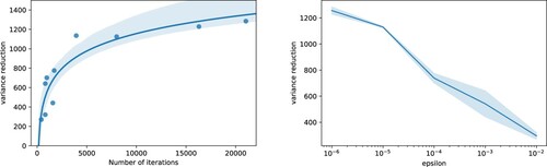
Figure A2. Number of optimizer iterations in terms of ϵ for Algorithm 3 used in Example A.1.

We note that in the example from Belomestny, Iosipoi, and Zhivotovskiy (2017, Sec 4.2.3), the control variate is trained with $S_0=0.7$ fixed. Using this setting, Algorithm 2 cannot be used to approximate the control variate in (9(9) $\begin{array}{rl}& {\mathcal{V}}^{\pi ,\theta ,\lambda ,N}(t,x;\text{β}):=\frac{1}{N}\sum _{i=1}^N\left\{\right(D^{\pi }(t,T){)}^{i}g\left(X_T^{\text{β},\pi ,i}\right)\phantom{\sum _{k=1}^{N_{\mathrm{s}\mathrm{t}\mathrm{e}\mathrm{p}\mathrm{s}}-1}}\\ & -\lambda \sum _{k=1}^{N_{\mathrm{s}\mathrm{t}\mathrm{e}\mathrm{p}\mathrm{s}}-1}\left(D^{\pi }\right(t,t_k\left){)}^i\mathcal{R}\right[{\mathrm{\partial }}_{x}v{]}_{\theta }(t_k,X_{t_k}^{\text{β},\pi ,i};\text{β})\sigma (t_k,X_{t_k}^{\text{β},\pi ,i};\text{β})(W_{t_{k+1}}^i-W_{t_k}^i)\},\end{array}$(9) ): since the network at t = 0, $\mathcal{R}[v{]}_{{\eta }_0}$, is trained only at $S_0=0.7$, then automatic differentiation to approximate ${\mathrm{\partial }}_x\mathcal{R}\left[v{]}_{{\eta }_0}\right(0.7)$ will yield a bad approximation of ${\mathrm{\partial }}_{x}v\left(0.7\right)$; indeed, during training $\mathcal{R}[v{]}_{{\eta }_0}$ is unable to capture how v changes around $S_0$ at t = 0. For this reason, Algorithm 2 is not included in the following results.

Example A.2

basket option with random sigma

In this example, as in Example 4.2, we aim to show how our approach – where we build a control variate by approximating the process $(Z_{t_k}{)}_{k=0,\dots ,N_{\mathrm{s}\mathrm{t}\mathrm{e}\mathrm{p}\mathrm{s}}}$ – is more robust compared to directly approximating the price by a certain function in a high-dimensional setting.

We use the methodology proposed in Blanka Horvath and Muguruza (2019), where the authors present a deep learning-based calibration method proposing a two-steps approach: first the authors learn the model that approximates the pricing map using an artificial neural network in which the inputs are the parameters of the volatility model. Second the authors calibrate the learned model using available data by means of different optimization methods.

For a fair comparison between our deep learning-based control variate approach vs. the method proposed in Blanka Horvath and Muguruza (2019), we make the following remarks:

1. We will only use the first step detailed in Blanka Horvath and Muguruza (2019) where the input to the model that approximates the pricing map is the volatility model's parameters: $\sigma \in {\mathbb{R}}^d,r$, and the initial price is considered constant for training purposes. We run the experiment for d = 5.

2. In Blanka Horvath and Muguruza (2019), the authors build a training set and then perform gradient descent-based optimization on the training set for a number of epochs. This is somewhat a limiting factor in the current setting where one can have as much data as they want since it is generated from some given distributions. In line with our experiments, instead of building a training set, in each optimization step we sample a batch from the given distributions.

3. In Blanka Horvath and Muguruza (2019), the price mapping function is learned for a grid of combinations of maturities and strikes. In this experiment, we reduce the grid to just one point considering T = 0.5, $K=\sum _i{S}_0^i$, where $S_0^i=0.7\mathrm{\forall }i$.

4. We will use Algorithm 3 to build the control variate with the difference that now $\sigma \in {\mathbb{R}}^d,r\in \mathbb{R}$ will be passed as input to the each network at each time step $\mathcal{R}[v{]}_{{\eta }_k},\mathcal{R}[{\mathrm{\partial }}_{x}v{]}_{{\theta }_k}$.

The experiment is organized as follows:

1. We train the network proposed in Blanka Horvath and Muguruza (2019) approximating the price using Black–Scholes model and Basket options payoff. In each optimization iteration, a batch of size $1000$, where the volatility model's parameters are sampled using $\sigma \sim \mathcal{U}(0.9,1.1)$ and $r\sim \mathcal{U}(0.4,0.6)$. We keep a test set of size 150, $\mathcal{S}=\left\{\right[({\sigma }^i,r^i);p({\sigma }^i,r^i)],i=1,\dots ,150\}$ where $p({\sigma }^i,r^i)$ denotes the price and is generated using 50, 000 Monte Carlo samples.

2. We use Algorithm 3 to build the control variate, where σ and r are sampled as above and are included as inputs to the network. We denote the trained model by $\mathcal{R}[{\mathrm{\partial }}_{x}v{]}_{{\theta }_k}$ where $k=1,\dots ,N_{\mathrm{s}\mathrm{t}\mathrm{e}\mathrm{p}\mathrm{s}}$. In contrast with Algorithm 3.

We present the following results:

1. Figure 1 displays the histogram of the squared error of the approximation of the PDE solution $\mathcal{R}[v{]}_{\eta }$ for each instance in $\mathcal{S}$. In this sample, it spans from almost ${10}^{-8}$ to ${10}^{-3}$ , i.e. ,for almost 5 orders of magnitude.

2. We build the control variate for that instance in the test set for which $\mathcal{R}[v{]}_{\eta }$ generalizes the worst. For those particular $\sigma ,r$, Table A3 provides its variance reduction factor.

Table E3. Results on basket options problem on 5 assets, Model trained with non-random $S_0$, and random $\sigma ,r$.

Method	Emp. Var.	Var. Red. Fact.
Monte Carlo	1.29	–
Algorithm 3	0.035	37

Example A.3

High dimensional basket option

We also consider the basket options problem on d = 100 assets but otherwise identical to the setting of Example A.1. We compare our results against the same experiment in Belomestny, Iosipoi, and Zhivotovskiy (2017, Sec 4.2.3, Table 6 and Table 7).

Table A4 shows a significant improvement of the variance reduction factor (10× and 100× better) of all our Algorithms than the methods proposed in Belomestny, Iosipoi, and Zhivotovskiy (2017) and applied in the same example.

Table E4. Results on basket options problem on 100 assets, Example A.3. Models trained with non-random $S_0$ so that the results can be directly compared to Belomestny, Iosipoi, and Zhivotovskiy (2017).

Method	Emp. Var.	Var. Red. Fact.	Train. Paths	Opt. Steps
Monte Carlo	79.83	–	–	–
Algorithm 3	$4.72\times {10}^{-4}$	168,952	$24\times {10}^7$	47,369
Algorithm 4	$1.79\times {10}^{-4}$	349,525	$37\times {10}^6$	7383
Algorithm 5	$1.54\times {10}^{-4}$	517,201	$35\times {10}^6$	7097
Method ${\zeta }_{\mathrm{a}}^1$ in Belomestny, Iosipoi, and Zhivotovskiy (2017)	$8.67\times {10}^{-1}$	97	–	–
Method ${\zeta }_{\mathrm{a}}^2$ in Belomestny, Iosipoi, and Zhivotovskiy (2017)	$4.7\times {10}^{-3}$	17,876	–	–

Table E5. Results on basket options problem on 100 assets, Example A.3. Models trained with non-random $S_0$.

Method	Confidence interval variance	Confidence interval estimator
Monte Carlo	$[8.57\times {10}^{-4},2.27\times {10}^{-3}]$	$[27.351,27.380]$
Monte Carlo + antithetic paths	$[5.34\times {10}^{-4},9.35\times {10}^{-4}]$	$[27.354,27.371]$
Algorithm 3	$[7.001\times {10}^{-9},1.8583\times {10}^{-8}]$	$[27.3692,27.3693]$
Algorithm 4	$[2.41\times {10}^{-9},6.39\times {10}^{-9}]$	$[27.36922,27.36928]$
Algorithm 5	$[4.1672\times {10}^{-9},1.1060\times {10}^{-8}]$	$[27.36922,27.36928]$

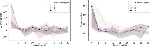
A.2. Empirical Network Diagnostics

In this section, we consider the exchange options problem on two assets from Example 4.1, where the time horizon is 1 day. We consider different network architectures for the BSDE method described by Algorithm 3 to understand their impact on the final result and their ability to approximate the solution of the PDE and its gradient. We choose this problem given the existence of an explicit solution that can be used as a benchmark. The experiment is organized as follows:

1. Let L−2 be the number of hidden layers of $\mathcal{R}[{\mathrm{\partial }}_{x}v{]}_{{\theta }_{t_0}}\in \mathcal{D}\mathcal{N}$ and $\mathcal{R}[v{]}_{{\theta }_{t_0}}\in \mathcal{D}\mathcal{N}$. Let $l_k$ be the number of neurones per hidden layer k.

2. We train four times all the possible combinations for $L-2\in \{1,2,3\}$ and for $l_k\in \{2,4,6,\dots ,20\}$ using $ϵ=5\times {10}^{-6}$ for the stopping criteria. The assets' initial values $s_{t_0}^i$ are sampled from a lognormal distribution $X\sim \exp \left(\right(\mu -0.5{\sigma }^2)\tau +\sigma \sqrt{\tau }\xi ),$ where $\xi \sim N(0,1),\mu =0.08,\tau =0.1$.

3. We approximate the $L^2$-error of $\mathcal{R}\left[v{]}_{{\theta }_{t_0}}\right(x)$ and $\mathcal{R}\left[v{]}_{{\theta }_{t_0}}\right(x)$ with respect to the exact solution given by Margrabe's formula and its gradient.

Figure A4 displays the average of the $L^2$-errors and its confidence interval. We can conclude that for this particular problem, the accuracy of $\mathcal{R}\left[v{]}_{{\theta }_{t_0}}\right(x)$ does not strongly depend on the number of layers, and that there is no improvement beyond eight nodes per hidden layer. The training (its inputs and the gradient descent algorithm together with the stopping criteria) becomes the limiting factor. The accuracy of $\mathcal{R}\left[v{]}_{{\theta }_{t_0}}\right(x)$ is clearly better with two or three hidden layers than with just one. Moreover, it seems that there is benefit in taking as many as 10 nodes per hidden layer.

Figure A3. Left: Variance reduction in terms of number of optimizer iterations. Right: Variance reduction in terms of epsilon. Both are for Example A.3 and Algorithm 3.

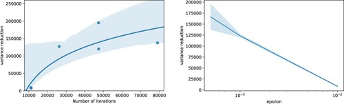
Figure A4. Average error of PDE solution approximation and its gradient and 95% confidence interval of different combination of # of layers and net width. Left: error model. Right: Error grad model.

References

- Bayer C., and B. Stemper. 2018. “Deep Calibration of Rough Stochastic Volatility Models.” arXiv:1810.03399.
- Beck C., S. Becker, P. Grohs, N. Jaafari, and A. Jentzen. 2018. “Solving Stochastic Differential Equations and Kolmogorov Equations by Means of Deep Learning.” arXiv:1806.00421.
- Beck C., L. Gonon, and A. Jentzen. 2020. “Overcoming the Curse of Dimensionality in the Numerical Approximation of High-Dimensional Semilinear Elliptic Partial Differential Equations”.
- Belomestny D., L. Iosipoi, and N. Zhivotovskiy. 2017. “Variance Reduction via Empirical Variance Minimization: Convergence and Complexity.” arXiv:1712.04667.
- Belomestny D., S. Hafner, T. Nagapetyan, and M. Urusov. 2018. “Variance Reduction for Discretised Diffusions Via Regression.” Journal of Mathematical Analysis and Applications 458 (1): 393–418.
- Berner J., P. Grohs, and A. Jentzen. January, 2020. “Analysis of the Generalization Error: Empirical Risk Minimization Over Deep Artificial Neural Networks Overcomes the Curse of Dimensionality in the Numerical Approximation of Black–scholes Partial Differential Equations.” SIAM Journal on Mathematics of Data Science 2 (3): 631–657.
- Blanka Horvath M. T., and Muguruza Aitor. 2019. “Deep Learning Volatility: A Deep Neural Network Perspective on Pricing and Alibration in (Rough) Volatility Models.” arXiv:1901.09647.
- M. Broadie, Y. Du, and C. C. Moallemi. 2015. “Risk Estimation Via Regression.” Operations Research 63 (5): 1077–1097.
- Chan-Wai-Nam Q., J. Mikael, and X. Warin. 2019. “Machine Learning for Semi Linear Pdes.” Journal of Scientific Computing 79 (3): 1667–1712.
- Chizat L., and F. Bach. 2018. “On the Global Convergence of Gradient Descent for Over-Parameterized Models Using Optimal Transport.” In Advances in Neural Information Processing Systems, 3036–3046.
- Cohen S. N., and R. J. Elliott. 2015. Stochastic Calculus and Applications. Vol. 2. New York: Birkhäuser.
- Cont R., and Y. Lu. March, 2016. “Weak Approximation of Martingale Representations.” Stochastic Processes and Their Applications 126 (3): 857–882.
- Cvitanic J., and J. Zhang. 2005. “The Steepest Descent Method for Forward-backward Sdes.” Electronic Journal of Probability 10: 1468–1495.
- Diederik J. B., and P. Kingma. 2017. “Adam: A Method for Stochastic Optimization.” arXiv:1412.6980.
- Du S. S., X. Zhai, B. Poczos, and A. Singh. 2018. “Gradient Descent Provably Optimizes Over-Parameterized Neural Networks.” arXiv:1810.02054.
- Elbrächter D., P. Grohs, A. Jentzen, and C. Schwab. Dnn expression rate analysis of high-dimensional pdes. 2022. “Application to Option Pricing.” Constructive Approximation 55 (1): 3–7.
- Glasserman P. 2013. Monte Carlo Methods in Financial Engineering. Springer.
- Gonon L., P. Grohs, A. Jentzen, D. Kofler, and D. Šiška. 2021. “Uniform Error Estimates for Artificial Neural Network Approximations for the Heat Equation.” IMA Journal Numerical Analysis. https://academic.oup.com/imajna/advance-article/doi/https://doi.org/10.1093/imanum/drab027/6279436?guestAccessKey=cef28afb-c79a-433a-855c-08f76b4732fd&login=false
- Goodfellow I., J. Shlens, and C. Szegedy. 2014. “Explaining and Harnessing Adversarial Examples.” arXiv:1412.6572.
- Grohs P., F. Hornung, A. Jentzen, and P. von Wurstemberger. 2018. “A Proof That Artificial Neural Networks Overcome the Curse of Dimensionality in the Numerical Approximation of Black-Scholes Partial Differential Equations.” arXiv:1809.02362.
- Grohs P., A. Jentzen, and D. Salimova. 2019. “Deep Neural Network Approximations for Monte Carlo Algorithms”.
- Han J., and J. Long. 2020. “Convergence of the Deep Bsde Method for Coupled Fbsdes.” Probability, Uncertainty and Quantitative Risk 5 (1): 1–33.
- Han J., A. Jentzen, and E. Weinan. 2017. “Solving High-Dimensional Partial Differential Equations Using Deep Learning.” arXiv:1707.02568.
- Henry-Labordere P. 2017. “Deep Primal-Dual Algorithm for BSDEs: Applications of Machine Learning to CVA and IM.” Available at SSRN 3071506.
- Hernandez A. 2016. “Model Calibration With Neural Networks.” Available at SSRN 2812140.
- Horvath B., A. Muguruza, and M. Tomas. 2019. “Deep Learning Volatility.” Available at SSRN 3322085.
- Hu K., Z. Ren, Šiška D., and L. Szpruch. 2021. “Mean-Field Langevin Dynamics and Energy Landscape of Neural Networks.” Annales de l'Institute Henry Poincaré Proability and Statistics 57 (4): 2043–2065.
- Huré C., H. Pham, and X. Warin. 2019. “Some Machine Learning Schemes for High-Dimensional Nonlinear PDEs.” arXiv:1902.01599.
- Hutzenthaler M., A. Jentzen, T. Kruse, and T. A. Nguyen. April, 2020. “A Proof that Rectified Deep Neural Networks Overcome the Curse of Dimensionality in the Numerical Approximation of Semilinear Heat Equations.” SN Partial Differential Equations and Applications 1 (2): 1–34.
- Itkin A. 2019. “Deep Learning Calibration of Option Pricing Models: Some Pitfalls and Solutions.” arXiv:1906.03507.
- Jacquier A. J., and M. Oumgari. 2019. “Deep PPDEs for Rough Local Stochastic Volatility.” Available at SSRN 3400035.
- Jentzen A., D. Salimova, and T. Welti. 2018. “A Proof That Deep Artificial Neural Networks Overcome the Curse of Dimensionality in the Numerical Approximation of Kolmogorov Partial Differential Equations With Constant Diffusion and Nonlinear Drift Coefficients.” arXiv:1809.07321.
- Krylov N. 1999. “On Kolmogorov's Equations for Finite Dimensional Diffusions.” In Stochastic PDE's and Kolmogorov Equations in Infinite Dimensions, 1–63. Springer.
- Krylov N. V. 2002. Introduction to the Theory of Random Processes. Vol. 43. American Mathematical Society.
- Kutyniok G., P. Petersen, M. Raslan, and R. Schneider. 2020. “A Theoretical Analysis of Deep Neural Networks and Parametric pdes”.
- LeCun Y., Y. Bengio, and G. Hinton. 2015. “Deep Learning.” Nature 521 (7553): 436.
- Liu S., A. Borovykh, L. A. Grzelak, and C. W. Oosterlee. 2019. “A Neural Network-Based Framework for Financial Model Calibration.” arXiv:1904.10523.
- McGhee W. A. 2018. “An Artificial Neural Network Representation of the SABR Stochastic Volatility Model.” SSRN 3288882.
- Mei S., A. Montanari, and P.-M. Nguyen. 2018. “A Mean Field View of the Landscape of Two-layer Neural Networks.” Proceedings of the National Academy of Sciences 115 (33): E7665–E7671.
- Milstein G., and M. Tretyakov. 2009. “Solving Parabolic Stochastic Partial Differential Equations Via Averaging Over Characteristics.” Mathematics of Computation 78 (268): 2075–2106.
- Newton N. J. 1994. “Variance Reduction for Simulated Diffusions.” SIAM Journal on Applied Mathematics 54 (6): 1780–1805.
- Øksendal B. 2003. “Stochastic Differential Equations.” In Stochastic Differential Equations, 65–84. Springer.
- Reisinger C., and Y. Zhang. 2020. “Rectified Deep Neural Networks Overcome the Curse of Dimensionality for Nonsmooth Value Functions in Zero-Sum Games of Nonlinear Stiff Systems”.
- Rotskoff G. M., and Vanden-Eijnden E.. 2018. “Neural Networks as Interacting Particle Systems: Asymptotic Convexity of the Loss Landscape and Universal Scaling of the Approximation Error.” arXiv:1805.00915.
- Sabate-Vidales M., D. Šiška, and L. Szpruch. 2020. “Solving Path Dependent pdes with LSTM Networks and Path Signatures”.
- Sergey Ioffe C. S. 2015. “Batch Normalization: Accelerating Deep Network Training by Reducing Internal Covariate Shift.” arXiv:1502.03167.
- Sirignano J., and K. Spiliopoulos. 2017. “DGM: A Deep Learning Algorithm for Solving Partial Differential Equations.” arXiv:1708.07469.
- Sirignano J., and K. Spiliopoulos. 2020. “Mean Field Analysis of Neural Networks: A Central Limit Theorem.” Stochastic Processes and Their Applications 130 (3): 1820–1852.
- Stone H. 2018. “Calibrating Rough Volatility Models: A Convolutional Neural Network Approach.” arXiv:1812.05315.
- Wang Z., and S. Tang. 2021. “Gradient Convergence of Deep Learning-based Numerical Methods for Bsdes.” Chinese Annals of Mathematics, Series B 42 (2): 199–216.
- Weinan E., J. Han, and A. Jentzen. 2017. “Deep Learning-based Numerical Methods for High-dimensional Parabolic Partial Differential Equations and Backward Stochastic Differential Equations.” Communications in Mathematics and Statistics 5 (4): 349–380.