The Impact of Stochastic Volatility on Initial Margin and MVA for Interest Rate Derivatives

ABSTRACT

In this research we investigate the impact of stochastic volatility on future initial margin (IM) and margin valuation adjustment (MVA) calculations for interest rate derivatives. An analysis is performed under different market conditions, namely during the peak of the Covid-19 crisis when the markets were stressed and during Q4 of 2020 when volatilities were low. The Cheyette short-rate model is extended by adding a stochastic volatility component, which is calibrated to fit the EUR swaption volatility surfaces. We incorporate the latest risk-free rate benchmarks (RFR), which in certain markets have been selected to replace the IBOR index. We extend modern Fourier pricing techniques to accommodate the RFR benchmark and derive closed-form sensitivity expressions, which are used to model IM profiles in a Monte Carlo simulation framework. The various results are compared to the deterministic volatility case. The results reveal that the inclusion of a stochastic volatility component can have a considerable impact on nonlinear derivatives, especially for far out-of-the-money swaptions. The effect is particularly pronounced if the market exhibits a substantial skew or smile in the implied volatility curve. This can have severe consequences for funding cost valuation and risk management.

KEYWORDS:

• Interest rate derivatives
• Cheyette
• initial margin
• MVA
• risk-free rates
• stochastic volatility

1. Introduction

The financial crisis of 2007–2008 led to a sharp increase in the default on debt and caused a near-collapse of the global banking system. In reaction to this crisis, regulators signed the Dodd-Frank act in 2010 and Basel III accords (Basel Committee on Banking Supervision 2010) in 2013 to bring stability to the financial system. It signified the importance of quantifying counterparty credit risk (CCR), the risk that the counterparty will default on the obligation and fail to fulfill its contractual agreements. In the years that followed the financial industry and regulators identified a number of valuation adjustments (xVA) to cover credit, funding and capital cost which financial institutions face in derivatives transactions (Gregory 2020). To limit the exposure to credit risk in over-the-counter (OTC) transactions, the regulator requires financial institutions to post two types of collateral. The first is called variation margin (VM), which is the part of the collateral that matches the loss of the current exposure of a portfolio. Since 2016, a second type of collateral has been introduced for OTC trades: initial margin (IM). This serves as a protection against exposure changes due to market moves in the margin period of risk, which is the time interval after a default when outstanding positions are not yet settled, but VM is not updated (Green 2015). Since 2021, IM has become compulsory for a large number of financial institutions. According to a report by the International Swaps and Derivatives Association (ISDA), the volume of collected IM for non-cleared derivatives transactions exceeded $200 billion by the end of 2020 (International Swaps and Derivatives Association, Inc 2021) and is only expected to further increase. In the pursuit of establishing a generic approach to IM valuation, ISDA has developed the Standard Initial Margin Model (SIMM,  International Swaps and Derivatives Association, Inc 2020). SIMM is a universal, sensitivity-based methodology for calculating initial margin requirements, which has become industry-standard across the bilateral OTC markets (Gregory 2020). The SIMM requirements are driven by the portfolio sensitivities to various risk-factors, including Delta-, Curvature- (Gamma) and Vega-risk. The cost of funding initial margin is called margin valuation adjustment (MVA) and is the latest addition to the xVA family. While other value adjustments such as CVA depend on the expected exposure, SIMM-based MVA requires trade sensitivities along the simulated paths, which poses a further computational challenge to the industry.

In the literature much attention is devoted to the mathematical characterization of dynamic IM and numerical methods that address the computational challenge of MVA valuation. In the work of Green and Kenyon (2015), MVA is characterized by extending the replication framework of Burgard and Kjaer (2013), to account for funding costs related to posting IM. They recognize that nested IM modelling may lead to an excessive computational burden and propose a least-square regression approach instead. In McWalter et al. (2018), a least-square method is used to capture IM as a (conditional) forward quantile of the portfolio value increments. In Biagini, Gnoatto, and Oliva (2019) and Biagini, Gnoatto, and Oliva (2021) it is shown that MVA can be characterized as a BSDE that is driven by a stochastic IM component. The work of  Garcia Trillos, Henrard, and Macrina (2016) captures MVA by modelling the expected shortfall of a derivative price increment as a stochastic process, driven by the underlying risk-factors. The publication of the ISDA SIMM methodology motivated many researchers to investigate efficient methods for forward sensitivity computation of financial derivatives, which is a challenging problem in itself. A technical, yet feasible method for fast sensitivity computation is adjoint algorithmic differention (AAD), which is applied in the context of SIMM in for example Antonov, Issakov, and McClelland (2017), Fries (2019) and Caspers and Lichters (2018). Other SIMM-based approximation schemes include least-square regression (Lakhany and Zhang 2021), spectral decomposition (Zeron and Ruiz 2018) and deep learning (Ma et al. 2019; Vierkoetter 2019).

In practice, risk-factors with immaterial impact are ignored or simplified to decrease the complexity of exposure and MVA computations. For instance, volatilities of interest rates are often assumed to be deterministic. However, various studies have shown that this assumption is unrealistic, as such models are unable to capture the smile or skew of the implied volatility curves that are observed in the interest rate markets (Andersen and Brotherton-Ratcliffe 2001; Collin-Dufresne and Goldstein 2002; Wu and Zhang 2006). An implication is that a model that is calibrated to at-the-money options, under- or overestimates in- and out-of-the-money options (Wu and Zhang 2006). In that extend, recent studies have shown that the inclusion or exclusion of stochastic volatility has a significant impact on the PFE of early-exercise equity options (De Graaf et al. 2014) and on expected exposure driving the CVA of FX derivatives (Simaitis et al. 2016). As initial margin reflects the tails of the risk-factor distribution, it is reasonable to expect a substantial impact for MVA as well. This may have severe implications for future IM valuation and risk management, which eventually could lead to collateral disputes.

In this work we contribute to the literature by studying the influence of the implied volatility skew on forward IM and MVA for various commonly traded interest rate derivatives. We do so by considering a short-rate model of Cheyette type (Cheyette 2001), which belongs to the HJM class and is Markovian. This model is extended with a stochastic volatility component in the spirit of Casassus, Collin-Dufresne, and Goldstein (2005). Using real market data we show that this model can achieve a satisfactory fit to the swaption volatility smiles, with only a small number of model parameters. To perform a representative study, the model is calibrated to the EUR 6M swaption market observed under two intrinsically different market conditions. The first data-set is extracted on 31 March 2020, at the peak of the Corona-crisis when markets were stressed. The second is extracted nine months later, when volatilites were low. Furthermore, we study the implications of a transition from LIBOR- to RFR-benchmarked derivatives. In certain markets, the LIBOR index will be discontinued is favour of short-term risk-free rates (RFR), such as SOFR, SONIA and ESTR. Where the LIBOR has a forward-looking nature (it fixes at the start of the accrual period), an RFR based term rate has a backward-looking nature (it compounds overnight and is set-in-arrears). The transition to an RFR benchmark will impact the valuation and modelling routines of several popular interest rate derivatives. For this study we take modern Fourier pricing techniques and extend them to accommodate backward-looking derivatives and negative rates. Additionally we derive closed-form sensitivity expressions, which serve as input to the ISDA SIMM calculations. Our analysis focusses on interest rate derivatives with the highest trading volumes: interest rate swaps, caps and vanilla swaptions. We consider Delta- and Vega- profiles, future IM and MVA, modelled with a Monte Carlo simulation framework. The impact of stochastic volatility is assessed by comparing to the Hull–White model (Hull and White 1990) with constant volatility and the implications of the LIBOR transform are studied by comparing to classic LIBOR derivatives.

The outline of this article is as follows. In Section 2 we introduce the main notation, the model specifications, the various derivatives and the risk-metrics of interest. The pricing and sensitivity routines that are used to compute margin profiles are described in Section 3. In Section 4 we present the market data and the model calibration procedure. The results of our experiments and corresponding analyses are subject of Section 5. We conclude in Section 6 by summarizing our findings.

2. Problem Formulation

In this section we will introduce the relevant definitions, models, derivatives and the risk-metrics of interest.

2.1. Definitions and Notation

We consider a continuous-time financial market, defined on a finite time horizon $[0,\overline{T}]$. Within the financial market we regard a money-market account where investments compound interest at a continuous, risk-free rate $r_t$. The process $M_t$ represents the time-t value of one unit of currency invested in the money-market at time-zero, given by $M_t={\mathrm{e}}^{{\int }_0^t{r}_u\mathrm{d}u},M_0=1$ Throughout this paper we will assume that $r_t$ represents the collateral rate used for discounting as well as the risk-free rate that is used to derive term rates. For RFR-benchmarked derivatives, this is consistent with the recent IBOR reform (Lyashenko and Mercurio 2019) and implies the return to a classic single-curve environment. However, for LIBOR-based derivatives this is a simplifying assumption, which has not been market practice since the 2007–08 financial crisis. Nonetheless we omit the embedding of a dual-curve framework for the sake of compactness and simplicity. We argue that the impact on the modelling of IM and MVA (see Section 2.4) is minimal, as the effect of bumping a risk-factor would be similar in both frameworks. Several tests under a single- and dual-curve environment have confirmed this (data not shown).

We let $(\mathrm{\Omega },\mathcal{F},\mathbb{P})$ denote a standard probability space representing the possible states of the economy and let $\{{\mathcal{F}}_t:0\le t\le \overline{T}\}$ be an augmented filtration generated by the Brownian motions driving the model risk-factors, representing the information generated by the economy up to time t. We further assume the existence of a risk-neutral measure $\mathbb{Q}$ equivalent to $\mathbb{P}$, under which securities denominated by the money-market numéraire are martingales. This condition is sufficient to guarantee that the market is free of arbitrage (Harrison and Pliska 1981).

A zero-coupon bond is a contract that guarantees the holder one unit of currency at maturity T. Throughout this work, we will use the notion of an extended zero-coupon bond, which is originally introduced in Lyashenko and Mercurio (2019). Consider the self-financing strategy that consists of holding a zero-coupon bond maturing at T and directly reinvesting the unit notional in the money-market upon maturity of the bond. The market value ${\hat{P}}_T$ of this strategy is given by (1) ${\hat{P}}_T\left(t\right)=\{\begin{array}{ll}{\displaystyle {\mathbb{E}}^{\mathbb{Q}}\left[{\mathrm{e}}^{-{\int }_t^T{r}_u\mathrm{d}u}|{\mathcal{F}}_t\right]}& \mathrm{i}\mathrm{f}0\le t<T\\ {\displaystyle {\mathrm{e}}^{{\int }_T^t{r}_u\mathrm{d}u}:=\frac{M_t}{M_T}}& \mathrm{i}\mathrm{f}T\le t\le \overline{T}\end{array}$(1) The the risk-neutral value of a traditional zero-coupon bond is equivalent to ${\hat{P}}_T$ if t<T. For the ease of notation we will hereafter, analogous to Lyashenko and Mercurio (2019), denote the time-t value of ${\hat{P}}_T$ as $P(t,T)$. We refer to $P(t,T)$ as the price of an extended zero-coupon bond. We let ${\mathbb{Q}}^T$ denote the extended T-forward measure equivalent to $\mathbb{P}$, under which securities denominated by ${\hat{P}}_T$ are martingales.

For the market term rates we will make a distinction between the classic, simply-compounded rates such as LIBOR and the new set-in-arrears rates based on the overnight risk-free benchmarks. The LIBOR $L(t,T)$ has a forward-looking nature as it fixes at some time t and represents the interest related to an investment over a subsequent accrual period $[t,T]$. In formulas we can write: $L(t,T):=\frac{1}{T-t}(\frac{1}{P(t,T)}-1)$ The set-in-arrears rate $R(t,T)$ has a backward-looking nature as it accrues over a period $[t,T]$ and the fixing value is only known by the end of that period, at time T. In formulas we can write: $R(t,T):=\frac{1}{T-t}(\frac{M_T}{M_t}-1)=\frac{1}{T-t}\left(P\right(T,t)-1)$ Finally we define a forward rate $F(\cdot ,T_0,T_1)$, which is the par rate of a forward-rate agreement (FRA) with expiry $T_0$ and maturity $T_1$, such that it has zero value at time t (Brigo and Mercurio 2006). By the no-arbitrage assumption, the forward rate is given by ${\mathbb{E}}^{T_1}\left[L\right(T_0,T_1\left)|{\mathcal{F}}_t\right]$ for classic forward-looking term rates and given by ${\mathbb{E}}^{T_1}\left[R\right(T_0,T_1\left)|{\mathcal{F}}_t\right]$ for the new backward-looking term rates. It is shown in Mercurio (2018) that when $t\le T_0$, the two forward rates coincide, i.e., ${\mathbb{E}}^{T_1}\left[R\right(T_0,T_1\left)|{\mathcal{F}}_t\right]={\mathbb{E}}^{T_1}\left[L\right(T_0,T_1\left)|{\mathcal{F}}_t\right],t<T_0$ Thus note that for both forward- and backward-looking rates, the classic expression for simply-compounded forward rates holds; given by (2) $F(t,T_0,T_1):=\frac{1}{T_1-T_0}(\frac{P(t,T_0)}{P(t,T_1)}-1)$(2) Moreover, for contracts written on in-arrears rates this expression remains valid during the accrual period $t\in [T_0,T_1]$, due to the extended bond price definition.

2.2. The Model

The new risk-free rate (RFR) benchmarks are short-term, overnight rates. When it comes to pricing and modelling RFR based derivates, instantaneous rate models therefore appear a natural choice. Well-known examples include instantaneous forward rate or short-rate models. The main model we use in this research is a two-factor short-rate model of Cheyette type. Cheyette models belong to the HJM class and are Markovian in a finite number of state-variables (Cheyette 2001). They can accommodate a large range of forward rate volatility structures, while maintaining computational tractability. The model of our choice can be considered an extension of the Hull–White model (Hull and White 1990), incorporating a stochastic volatility component. Assuming a stochastic volatility allows to capture the volatility smile or skew that is typically observed in the swaption market. Similar models have been studied in for example Casassus, Collin-Dufresne, and Goldstein (2005) and Trolle and Schwartz (2009). The risk-neutral dynamics of the $\mathbb{R}$-valued state-variables are given by (3) $\begin{array}{rl}& r_t:=f(t,t)=x_t+f(0,t)\end{array}$(3) (4) $\begin{array}{rl}& \mathrm{d}{x}_t=({\varphi }_t-a{x}_t)\mathrm{d}t+\sqrt{v_t}\mathrm{d}{W}_t,x_0=0\end{array}$(4) (5) $\begin{array}{rl}& \mathrm{d}{\varphi }_t=(v_t-2a{\varphi }_t)\mathrm{d}t,{\varphi }_0=0\end{array}$(5) (6) $\begin{array}{rl}& \mathrm{d}{v}_t=\kappa (\overline{v}-v_t)\mathrm{d}t+ϵ\sqrt{v_t}\mathrm{d}{Z}_t,v_0=v\end{array}$(6) (7) $\begin{array}{rl}& d{〈W,Z〉}_t=\rho \mathrm{d}t\end{array}$(7) The process $x_t$ models the spread between the short-rate $r_t$ and the initial instantaneous forward rate $f(0,t)$. It is modelled as a mean-reverting process, with mean-reversion rate a. The volatility follows a square-root process, with mean-reversion rate κ, long-term mean $\overline{v}$ and vol-of-vol ε. The standard $\mathbb{Q}$ Brownian motions W and Z are assumed to have constant correlation ρ. The state-variable ϕ represents the integrated variance of the instantaneous forward rate and is defined by ${\varphi }_t:={\int }_0^t{\mathrm{e}}^{-2a(t-u)}{v}_u\mathrm{d}u$. Given the state of the variables $r_t$ and ${\varphi }_t$, the entire term-structure can be reconstructed  (Ritchken and Sankarasubramanian 1995). As the state-variables define a Markovian, affine term-structure model, it admits explicit zero-coupon bond prices. Define the function $B(\cdot ,T)$ as (8) $B(t,T):=\frac{1}{a}(1-{\mathrm{e}}^{-a(T-t)})$(8) The bond price $P(t,T)$ prevailing at time t and maturing at time T (assuming t<T) is given by (9) $P(t,T)=\frac{P(0,T)}{P(0,t)}\exp \{-\frac{1}{2}{B}^2(t,T){\varphi }_t-B(t,T\left)x_t\right\}$(9) We refer to Brigo and Mercurio (2006), Ritchken and Sankarasubramanian (1995) and Filipovic (2009) for details.

To investigate the impact of the stochastic volatility component, we consider a standard one-factor Hull–White model (Hull and White 1990) with constant, deterministic volatility σ as a benchmark. This model can be considered a special case of the Cheyette model presented in (3(3) $\begin{array}{rl}& r_t:=f(t,t)=x_t+f(0,t)\end{array}$(3) )–(7(7) $\begin{array}{rl}& d{〈W,Z〉}_t=\rho \mathrm{d}t\end{array}$(7) ). It is obtained by setting $v_0:={\sigma }^2$ and $\kappa =ϵ:=0$, and thus ${\varphi }_t:=\frac{{\sigma }^2}{2a}(1-{\mathrm{e}}^{-2at})$.

2.3. Derivatives

This study considers interest rate swaps, caps and vanilla swaptions. Under the assumption that discount factors and term rates are implied by a single-curve term-structure, we obtain the classic textbook valuation formulas for the LIBOR-based derivatives. This has the advantage of more tractable pricing and sensitivity expressions and has only a minor impact on the modelling results. For swaps and caps an explicit distinction will be made between the RFR-based and the LIBOR-based derivative. The valuation of an RFR swaption is in this case equivalent to the LIBOR swaption and will therefore not be treated separately.

2.3.1. Interest Rate Swap

An interest rate swap is a contract that exchanges interest payments between two parties (Brigo and Mercurio 2006). Swaps are particularly relevant in the light of CCR due to their high trading volumes in the OTC market. In 2020, the global outstanding notional amounts well exceeded 300 Trillion US Dollar (Bank for International Settlements 2021), making it by far the most traded OTC interest rate derivative. In this study we consider fixed-floating payer swaps, where the holder receives floating interest on dates $T_1,\dots ,T_M$ and pays a fixed rate K on dates $T_1^{\mathrm{\prime }},\dots ,T_{M^{\mathrm{\prime }}}^{\mathrm{\prime }}$. We assume a unit notional, let ${\tau }_j$ denote the year-fraction $T_j-T_{j-1}$ and similarly let ${\tau }_j^{\mathrm{\prime }}$ denote the year-fraction $T_j^{\mathrm{\prime }}-T_{j-1}^{\mathrm{\prime }}$. Let $T_0=T_0^{\mathrm{\prime }}$ and $T_M=T_{M^{\mathrm{\prime }}}^{\mathrm{\prime }}$. At times $t<T_0$, RFR swaps and LIBOR swaps have an equivalent value $V\left(t\right)$, given by (10) $V\left(t\right)=P(t,T_0)-P(t,T_M)-\sum _{m=1}^{M^{\mathrm{\prime }}}{\tau }_j^{\mathrm{\prime }}KP(t,T_m^{\mathrm{\prime }})$(10) However, at any time after the inception date a distinction needs to be made. Let $T_{i-1}<t<T_i$ and $T_{j-1}^{\mathrm{\prime }}<t<T_j^{\mathrm{\prime }}$, then the swap values are given by (11) $V\left(t\right)=\{\begin{array}{ll}{\displaystyle \frac{P(t,T_i)}{P(T_{i-1},T_i)}-P(t,T_M)-\sum _{m=j}^{M^{\mathrm{\prime }}}{\tau }_j^{\mathrm{\prime }}KP(t,T_m^{\mathrm{\prime }})}& \mathrm{L}\mathrm{I}\mathrm{B}\mathrm{O}\mathrm{R}\mathrm{s}\mathrm{w}\mathrm{a}\mathrm{p}\\ {\displaystyle \frac{M_t}{M_{T_{i-1}}}-P(t,T_M)-\sum _{m=j}^{M^{\mathrm{\prime }}}{\tau }_j^{\mathrm{\prime }}KP(t,T_m^{\mathrm{\prime }})}& \mathrm{R}\mathrm{F}\mathrm{R}\mathrm{s}\mathrm{w}\mathrm{a}\mathrm{p}\end{array}$(11) where the difference originates from the fact that the first upcoming floating coupon is already fixed in the LIBOR case, but is still accruing in the RFR case.

2.3.2. Interest Rate Cap

A cap is a contract in which a series of interest payments are exchanged between two parties, but each contingent on the amount by which the floating rate exceeds a fixed rate (Brigo and Mercurio 2006). A cap can therefore be decomposed in a series of options, known as caplets. Here we will consider cap contracts with equidistant tenor structures, denoted as $T_0,\dots ,T_M$. We again assume unit notional amounts and let K denote the fixed cap rate. We say a cap is at-the-money (ATM) if K is equal to the prevailing swap rate (12) $S_{0,M}\left(t\right):=\frac{P(t,T_0)-P(t,T_M)}{\sum _{m=1}^M{\tau }_{m}P(t,T_m)},t<T_0$(12) We will again distinguish between a forward-looking and a backward-looking contract. In the former, the floating rate is set in-advance, which yields a caplet pay-off given by ${\tau }_j\left(L\right(T_{j-1},T_j)-K{)}^{+}$. In the latter, the floating rate is set in-arrears, which yields a caplet pay-off given by ${\tau }_j\left(R\right(T_{j-1},T_j)-K{)}^{+}$. As RFR caplets expire at the end of the accrual period, its pay-off has a larger variance than that of a classic LIBOR caplet, which expires at the start of the accrual period. For this reason, RFR caps have by definition a higher value than LIBOR caps, as is shown in Lyashenko and Mercurio (2019). If $t<T_{j-1}$, the LIBOR caplet value (see also Filipovic 2009) is given by (13) $\begin{array}{rl}V\left(t\right)& ={\mathbb{E}}^{\mathbb{Q}}\left[{\mathrm{e}}^{-{\int }_t^{T_j}{r}_u\mathrm{d}u}{\tau }_j{(L(T_{j-1},T_j)-K)}^{+}|{\mathcal{F}}_t\right]\end{array}$(13) (14) $\begin{array}{rl}& ={\mathbb{E}}^{\mathbb{Q}}\left[{\mathrm{e}}^{-{\int }_t^{T_{j-1}}{r}_u\mathrm{d}u}(1+{\tau }_{j}K){(\frac{1}{1+{\tau }_{j}K}-P(T_{j-1},T_j\left)\right)}^{+}|{\mathcal{F}}_t\right]\end{array}$(14) (15) $\begin{array}{rl}& =K_{j}P(t,T_{j-1}){\mathbb{E}}^{T_{j-1}}\left[{(\frac{1}{K_j}-P(T_{j-1},T_j\left)\right)}^{+}|{\mathcal{F}}_t\right]\end{array}$(15) and if $t<T_j$, the RFR caplet value $V\left(t\right)$ is given by (16) $\begin{array}{rl}V\left(t\right)& ={\mathbb{E}}^{\mathbb{Q}}\left[{\mathrm{e}}^{-{\int }_t^{T_j}{r}_u\mathrm{d}u}{\tau }_j{(R(T_{j-1},T_j)-K)}^{+}|{\mathcal{F}}_t\right]\end{array}$(16) (17) $\begin{array}{rl}& ={\mathbb{E}}^{\mathbb{Q}}\left[{\mathrm{e}}^{-{\int }_t^{T_j}{r}_u\mathrm{d}u}{\left(P\right(T_j,T_{j-1})-1-{\tau }_{j}K)}^{+}|{\mathcal{F}}_t\right]\end{array}$(17) (18) $\begin{array}{rl}& =P(t,T_j){\mathbb{E}}^{T_j}\left[{\left(P\right(T_j,T_{j-1})-K_j)}^{+}|{\mathcal{F}}_t\right]\end{array}$(18) where in both expressions we denoted $K_j:=1+{\tau }_{j}K$, assuming $K>-\frac{1}{{\tau }_j}$.

2.3.3. Swaption

A swaption is a contract, that gives the holder the right to enter an interest rate swap on a specified future date at a fixed rate K  (Brigo and Mercurio 2006). We will consider European payer swaptions, where the underlying swap exchanges floating interest on dates $T_1,\dots ,T_M$ versus fixed rate payments on dates $T_1^{\mathrm{\prime }},\dots ,T_{M^{\mathrm{\prime }}}^{\mathrm{\prime }}$. We assume that the swaption expiry coincides with the first fixing date of the swap (i.e., $T_0$). As the contract matures before the inception of the first accrual period of the underlying swap, the pay-off of an RFR swaption is equivalent to that of a classic LIBOR swaption. With a unit notional, its value for $t<T_0$ (see Filipovic 2009) is given by (19) $V\left(t\right)=\sum _{m=1}^{M^{\mathrm{\prime }}}{\tau }_m^{\mathrm{\prime }}P(t,T_m^{\mathrm{\prime }}){\mathbb{E}}^{0,M}\left[{\left(S_{0,M}\right(T_0)-K)}^{+}|{\mathcal{F}}_t\right]$(19) where the expectation above is taken under the annuity measure ${\mathbb{Q}}^{0,M}$ associated with the annuity numéraire, defined as $A_{0,M}\left(t\right):=\sum _{m=1}^{M^{\mathrm{\prime }}}{\tau }_m^{\mathrm{\prime }}P(t,T_m^{\mathrm{\prime }})$. We say a swaption is at-the-money at time t if $K=S_{0,M}\left(t\right)$.

In the subsequent sections we will repeatedly refer to normal implied swaption volatility, for which we will now provide a definition. Under the assumption that the swap rate process is captured by an arithmetic Brownian motion, with constant volatility $\sigma >0$, the future swap rate is normally distributed. In that case the risk-neutral value of a swaption at $t<T_0$ can be computed using Bachelier's option pricing formula  (Musiela and Rutkowski 1997), given by (20) $\begin{array}{rl}{V}_{\mathrm{B}\mathrm{a}\mathrm{c}\mathrm{h}}(t,\sigma ,K)& =A_{0,M}\left(t\right)[\omega \left(S_{0,M}\right(t)-K)\mathrm{\Phi }\left(\omega d\right)+\sigma \sqrt{T_0-t}\cdot \phi \left(d\right)]\end{array}$(20) (21) $\begin{array}{rl}d& =\frac{S_{0,M}\left(t\right)-K}{\sigma \sqrt{T_0-t}}\end{array}$(21) where φ and Φ denote the standard normal PDF and CDF, respectively, and ω distiguishes between a payer $(\omega =1)$ and receiver $(\omega =-1)$ swaption. We define the normal implied swaption volatility at date t associated to the option written on the swap rate $S_{0,M}$ with strike K and market price $\tilde{V}$ as the positive scalar ${\sigma }_{\mathrm{i}\mathrm{m}\mathrm{p}}$, which solves the equation $V_{\mathrm{B}\mathrm{a}\mathrm{c}\mathrm{h}}(t,{\sigma }_{\mathrm{i}\mathrm{m}\mathrm{p}},K)=\tilde{V}$ Throughout the remainder of this text we will simply refer to this quantity as the implied volatility.

2.4. Initial Margin and MVA

Initial margin (IM) is a type of collateral, which serves as a protection against exposure changes due to market moves in the margin period of risk. Specifically, IM is meant to cover against a potential increase in exposure over a 10 days close-out period, with a confidence level of 99%  (Gregory 2020). The close-out period is the time interval between the event of default and the settlement of the outstanding positions, when variation margin (VM) is no longer updated. The industry-standard methodology for calculating bilateral IM is the Standard Initial Margin Model (SIMM) developed by ISDA. SIMM is a quantitative approach for evaluating margin requirements, which is driven by the sensitivities of a trade to potential market moves. Delta risk represents the sensitivity of a derivative to the underlying (in our case the interest rates), Curvature risk is the second-order sensitivity to the underlying (Gamma) and Vega risk represents the sensitivity to changes in the implied volatility surface. For the purpose of this article we only provide a basic overview of SIMM, restricted to single-currency IR derivative portfolios. Details of the methodology can be found in  International Swaps and Derivatives Association, Inc (2020).

The SIMM methodology distinguishes four product classes, in which each product is exposed to risk that can be decomposed into six risk classes. In this study we will only consider portfolios of single interest rate derivatives in a single currency, written on a single interest rate curve. Therefore, the RatesFX class, which represents IR and FX derivatives, is the only relevant product class. Likewise, the interest rate risk class, which represents exposure to interest rate risk, is the only relevant risk class. The total IM is defined by the following sum: (22) $\mathrm{I}\mathrm{M}\left(t\right)=\sum _{g\in \mathcal{G}}{\mathrm{M}\mathrm{a}\mathrm{r}\mathrm{g}\mathrm{i}\mathrm{n}}_g\left(t\right),\mathcal{G}=\left\{\mathrm{D}\mathrm{e}\mathrm{l}\mathrm{t}\mathrm{a},\mathrm{V}\mathrm{e}\mathrm{g}\mathrm{a},\mathrm{C}\mathrm{u}\mathrm{r}\mathrm{v}\mathrm{a}\mathrm{t}\mathrm{u}\mathrm{r}\mathrm{e}\right\}$(22) Each margin component captures the risk of exposure change due to an up or down movement of an underlying risk-factor. A portfolio's sensitivity to risk-factor movements depends on the state of the economy, which implies that $\left\{\mathrm{I}\mathrm{M}\right(t):0\le t\le \overline{T}\}$ is a stochastic process.

A margin component (i.e., Delta, Vega or Curvature) is explicitly calculated using a variance/covariance formula (International Swaps and Derivatives Association, Inc 2016). Let $\mathbf{\Delta }\mathbf{Y}$ denote a d-dimensional random vector, which represents the 10-day evolution of the underlying market risk-factors and let $\mathbf{\Sigma }$ denote the covariance matrix of $\mathbf{\Delta }\mathbf{Y}$. Furthermore, let ${\mathrm{\partial }}_{i}V:=\frac{\mathrm{\partial }V}{\mathrm{\partial }{Y}_i}$ denote the sensitivity of the instrument to a small change in the risk-factor $Y_i$. Assuming $\mathbf{\Delta }\mathbf{Y}$ has zero mean and is by approximation normal, the 10-day ${\mathrm{V}\mathrm{a}\mathrm{R}}_{99\mathrm{\%}}$ of the product's exposure due to changes in market risk-factor $\mathbf{Y}$ can be captured by ${\mathrm{V}\mathrm{a}\mathrm{R}}_{99\mathrm{\%}}\approx {\mathrm{\Phi }}^{-1}\left(99\mathrm{\%}\right)\sqrt{{\left(\mathrm{\partial }\mathbf{V}\right)}^{\mathrm{\top }}\mathbf{\Sigma }\mathrm{\partial }\mathbf{V}}$ where ${\mathrm{\Phi }}^{-1}$ denotes the inverse of the standard normal distribution function. Defining a risk weight as $R{W}_i:={\sigma }_i{\mathrm{\Phi }}^{-1}\left(99\mathrm{\%}\right)$, with ${\sigma }_i$ denoting the standard deviation of $\mathrm{\Delta }{Y}_i$, the expression above can be rewritten into an expression for each margin component, i.e., (23) ${\mathrm{M}\mathrm{a}\mathrm{r}\mathrm{g}\mathrm{i}\mathrm{n}}_g\left(t\right)=\sqrt{\sum _{i=1}^d{\mathrm{R}\mathrm{W}}_i^2{\left({\mathrm{\partial }}_{g,i}V\right(t\left)\right)}^2+\sum _{i=1}^d\sum _{j\ne i}{\rho }_{ij}{\mathrm{R}\mathrm{W}}_i{\mathrm{R}\mathrm{W}}_j{\mathrm{\partial }}_{g,i}V\left(t\right){\mathrm{\partial }}_{g,j}V\left(t\right)}$(23) The factor ${\rho }_{ij}$ denotes the correlation between $\mathrm{\Delta }{Y}_i$ and $\mathrm{\Delta }{Y}_j$. The risk weights and correlations are fixed scalars that are periodically published by ISDA, leaving only the sensitivities to be evaluated by the financial institution. We specify the relevant sensitivity vectors ${\mathrm{\partial }}_{g}V$ for each margin component below:

• The Delta margin requires sensitivities taken against quoted market rates (e.g., swap rates) with given tenors $\mathcal{K}=\left\{2\mathrm{W},1\mathrm{M},3\mathrm{M},6\mathrm{M},1\mathrm{Y},2\mathrm{Y},3\mathrm{Y},5\mathrm{Y},10\mathrm{Y},15\mathrm{Y},20\mathrm{Y},30\mathrm{Y}\right\}$. We denote the Delta risk (DR) vector as ${\mathrm{\partial }}_{\mathrm{D}\mathrm{e}\mathrm{l}\mathrm{t}\mathrm{a}}V\left(t\right):=[\frac{\mathrm{\partial }V\left(t\right)}{\mathrm{\partial }{S}_{2\mathrm{W}}}\cdots \frac{\mathrm{\partial }V\left(t\right)}{\mathrm{\partial }{S}_{30\mathrm{Y}}}]$ in which $S_{\tau }$ denotes the par rate of a swap with tenor $\tau \in \mathcal{K}$.

• The Vega margin requires sensitivities taken against implied at-the-money volatilities of swaptions with expiry times equal to tenors $\mathcal{K}$. The volatilities can be quoted as normal or log-normal volatilities. To align the normal and log-normal quotes, each sensitivity is scaled with the implied volatility itself. We denote the Vega risk (VR) vector as ${\mathrm{\partial }}_{\mathrm{V}\mathrm{e}\mathrm{g}\mathrm{a}}V\left(t\right):=[{\sigma }_{2\mathrm{W}}\frac{\mathrm{\partial }V\left(t\right)}{\mathrm{\partial }{\sigma }_{2\mathrm{W}}}\cdots {\sigma }_{30\mathrm{Y}}\frac{\mathrm{\partial }V\left(t\right)}{\mathrm{\partial }{\sigma }_{30\mathrm{Y}}}]$

• For Curvature margin, the Gamma sensitivities are approximated using the Vega-Gamma relationship of Black's model  (International Swaps and Derivatives Association, Inc 2016). The Vega sensitivities are therefore also used as an input to estimate Curvature margin. We denote the Curvature risk (CVR) vector as $\begin{array}{rl}{\mathrm{\partial }}_{\mathrm{C}\mathrm{u}\mathrm{r}\mathrm{v}\mathrm{a}\mathrm{t}\mathrm{u}\mathrm{r}\mathrm{e}}V\left(t\right)& :=\left[\mathrm{S}\mathrm{F}\right(2\mathrm{W}){\sigma }_{2\mathrm{W}}\frac{\mathrm{\partial }V\left(t\right)}{\mathrm{\partial }{\sigma }_{2\mathrm{W}}}\cdots {\displaystyle \mathrm{S}\mathrm{F}\left(30\mathrm{Y}\right){\sigma }_{30\mathrm{Y}}\frac{\mathrm{\partial }V\left(t\right)}{\mathrm{\partial }{\sigma }_{30\mathrm{Y}}}}],\\ \mathrm{S}\mathrm{F}\left(\tau \right)& :=0.5min\{1,\frac{14}{\tau }\}\end{array}$ where τ is the number of days to expiry of each standard option with tenor $k\in \mathcal{K}$.

In contrast to VM, IM typically cannot be rehypothecated. For this reason IM needs to be funded by the dealer. Let $\mathrm{I}\mathrm{M}\left(t\right)$ denote the initial margin posted against a financial contract at future date t. Expected initial margin (EIM) is defined as $\mathrm{E}\mathrm{I}\mathrm{M}\left(t\right):={\mathbb{E}}^{\mathbb{Q}}\left[{\mathrm{e}}^{-{\int }_0^t{r}_u\mathrm{d}u}\mathrm{I}\mathrm{M}\right(t\left)|{\mathcal{F}}_0\right]$ Expected IM is a key ingredient for computing the funding cost related to posting IM. The expected lifetime cost of posting IM against a portfolio is called Margin Valuation Adjustment (MVA). Assuming the funding spread related to the margin is independent of its size, MVA can be computed as Green and Kenyon (2015) (24) $\mathrm{M}\mathrm{V}\mathrm{A}={\int }_0^T\mathrm{F}\mathrm{S}\left(u\right)\mathrm{E}\mathrm{I}\mathrm{M}\left(u\right)\mathrm{d}u\approx \sum _{i=1}^n\mathrm{F}\mathrm{S}\left(t_i\right)\times \mathrm{E}\mathrm{I}\mathrm{M}\left(t_i\right)\times (t_i-t_{i-1})$(24) with FS denoting the funding spread, reflecting the margin type, the spread on IM and any related renumeration or repo rate (Gregory 2020). For details we refer to Green and Kenyon (2015).

3. Pricing and Sensitivity Computation

In this section we describe the routines to compute prices and sensitivities of the selected derivatives. We assume the dynamics of the risk-factors are captured by the Cheyette stochastic volatility model as described in Equations (4(4) $\begin{array}{rl}& \mathrm{d}{x}_t=({\varphi }_t-a{x}_t)\mathrm{d}t+\sqrt{v_t}\mathrm{d}{W}_t,x_0=0\end{array}$(4) )–(7(7) $\begin{array}{rl}& d{〈W,Z〉}_t=\rho \mathrm{d}t\end{array}$(7) ). For brevity we will limit the exposition to the backward-looking derivatives where relevant. The calculations for the forward-looking variants can be derived in the same spirit.

3.1. Cap Pricing

The routine for pricing a cap is a generalization of the work of Casassus, Collin-Dufresne, and Goldstein (2005) and Trolle and Schwartz (2009). Their methodology is extended to accommodate for both forward- and backward-looking caps. Here we will focus on the price of an RFR caplet, which is equivalent to a call option on an extended zero-coupon bond, see (16(16) $\begin{array}{rl}V\left(t\right)& ={\mathbb{E}}^{\mathbb{Q}}\left[{\mathrm{e}}^{-{\int }_t^{T_j}{r}_u\mathrm{d}u}{\tau }_j{(R(T_{j-1},T_j)-K)}^{+}|{\mathcal{F}}_t\right]\end{array}$(16) ). For $t<T_j$, it is given by: (25) $V\left(t\right)={\mathbb{E}}^{\mathbb{Q}}\left[{\mathrm{e}}^{-{\int }_t^{T_j}{r}_u\mathrm{d}u}{\left(P\right(T_j,T_{j-1})-K_j)}^{+}|{\mathcal{F}}_t\right]={\mathrm{\Psi }}_1(t,K_j)-K_j{\mathrm{\Psi }}_0(t,K_j)$(25) in which, for $a\in \{0,1\}$, (26) ${\mathrm{\Psi }}_a(t,K_j):={\mathbb{E}}^{\mathbb{Q}}\left[{\mathrm{e}}^{-{\int }_t^{T_j}{r}_u\mathrm{d}u}{\mathrm{e}}^{a\log P(T_j,T_{j-1})}{\mathbb{1}}_{\{\log K_j<\log P(T_j,T_{j-1}\left)\right\}}|{\mathcal{F}}_t\right]$(26) Note that the caplet does not expire until the end of the accrual period at time $T_j$ and therefore yields a higher implied volatility than a forward-looking caplet. The value of ${\mathrm{\Psi }}_a$ can be analytically derived by considering a measure change, implied by the Radon–Nikodym derivative $\frac{\mathrm{d}\stackrel{\mathbb{~}}{\mathbb{Q}}}{\mathrm{d}\mathbb{Q}}:={\mathrm{e}}^{-{\int }_0^{T_j}{r}_u\mathrm{d}u}{\mathrm{e}}^{a\log P(T_j,T_{j-1})}$. The related Radon–Nikodym process is represented by the following transform (27) $\psi (\omega ,t)={\mathbb{E}}^{\mathbb{Q}}[{\mathrm{e}}^{-{\int }_t^{T_j}{r}_u\mathrm{d}u}\exp \{\omega \log P(T_j,T_{j-1}\left)\right\}|{\mathcal{F}}_t]$(27) for some complex variable ω. The Radon–Nikodym process allows us to rewrite the conditional expectation in (26(26) ${\mathrm{\Psi }}_a(t,K_j):={\mathbb{E}}^{\mathbb{Q}}\left[{\mathrm{e}}^{-{\int }_t^{T_j}{r}_u\mathrm{d}u}{\mathrm{e}}^{a\log P(T_j,T_{j-1})}{\mathbb{1}}_{\{\log K_j<\log P(T_j,T_{j-1}\left)\right\}}|{\mathcal{F}}_t\right]$(26) ) as ${\mathrm{\Psi }}_a(t,K_j)=\psi (a,t){\mathbb{E}}^{\stackrel{\mathbb{~}}{\mathbb{Q}}}\left[{\mathbb{1}}_{\{\log K_j<\log P(T_j,T_{j-1}\left)\right\}}|{\mathcal{F}}_t\right]$. This measure-changed expression can be evaluated using a Fourier inversion technique. In that regard, note that the characteristic function of $X:=\log P(T_j,T_{j-1})$ can be written as ${\phi }_X(u,t):={\mathbb{E}}^{\stackrel{\mathbb{~}}{\mathbb{Q}}}\left[{\mathrm{e}}^{iuX}|{\mathcal{F}}_t\right]=\frac{\psi (a+iu,t)}{\psi (a,t)}$. An application of the Gil-Pelaez theorem then yields ${\mathrm{\Psi }}_a(t,K_j)=\frac{\psi (a,t)}{2}+\frac{1}{\pi }{\int }_0^{\mathrm{\infty }}\frac{\mathrm{I}\mathrm{m}\left[\psi \right(a+iu,t\left){\mathrm{e}}^{-iu\log K_j}\right]}{u}\mathrm{d}u$ Numerically evaluating the expression above for a = 0, 1 and substitution in (25(25) $V\left(t\right)={\mathbb{E}}^{\mathbb{Q}}\left[{\mathrm{e}}^{-{\int }_t^{T_j}{r}_u\mathrm{d}u}{\left(P\right(T_j,T_{j-1})-K_j)}^{+}|{\mathcal{F}}_t\right]={\mathrm{\Psi }}_1(t,K_j)-K_j{\mathrm{\Psi }}_0(t,K_j)$(25) ), produces the required option price. The following proposition provides a (semi) closed-form expression for the transform in (27(27) $\psi (\omega ,t)={\mathbb{E}}^{\mathbb{Q}}[{\mathrm{e}}^{-{\int }_t^{T_j}{r}_u\mathrm{d}u}\exp \{\omega \log P(T_j,T_{j-1}\left)\right\}|{\mathcal{F}}_t]$(27) ). A proof is given in Appendix 1.

Proposition 3.1

The transform given in (27(27) $\psi (\omega ,t)={\mathbb{E}}^{\mathbb{Q}}[{\mathrm{e}}^{-{\int }_t^{T_j}{r}_u\mathrm{d}u}\exp \{\omega \log P(T_j,T_{j-1}\left)\right\}|{\mathcal{F}}_t]$(27) ) admits the solution $\psi (\omega ,t)=\exp \left\{C\right(t)+D(t)v_t+\omega \log P(t,T_{j-1})+(1-\omega )\log P(t,T_j\left)\right\}$ where the deterministic functions $C(\cdot ),D(\cdot )$ satisfy the system of ODEs given by $\begin{array}{rl}\frac{\mathrm{d}C\left(t\right)}{\mathrm{d}t}& =-D\left(t\right)\kappa \overline{v}\\ \frac{\mathrm{d}D\left(t\right)}{\mathrm{d}t}& =(\phantom{|}\kappa +ϵ\rho \left(\omega B\right(t,T_{j-1}){\mathbb{1}}_{\{t\le T_{j-1}\}}+(1-\omega \left)B\right(t,T_j\left){\mathbb{1}}_{\{t\le T_j\}}\right))D\left(t\right)\\ & -\frac{1}{2}{ϵ}^{2}D(t{)}^2+\frac{1}{2}\omega (1-\omega ){\left(B\right(t,T_{j-1}){\mathbb{1}}_{\{t\le T_{j-1}\}}-B(t,T_j\left){\mathbb{1}}_{\{t\le T_j\}}\phantom{|}\right)}^2\end{array}$ with terminal conditions $C\left(T_j\right)=D\left(T_j\right)=0$.

The proof, which is a generalization of the one given in Casassus, Collin-Dufresne, and Goldstein (2005) and Trolle and Schwartz (2009), relies on the insight that the extended bond price $P(\cdot ,T)$ has the following risk-neutral dynamics (see Lyashenko and Mercurio 2019): $\frac{\mathrm{d}P(t,T)}{P(t,T)}=r_t\mathrm{d}t-B(t,T)\sqrt{v_t}{\mathbb{1}}_{\{t\le T\}}\mathrm{d}{W}_t$ where $B(\cdot ,T)$ is as in (8(8) $B(t,T):=\frac{1}{a}(1-{\mathrm{e}}^{-a(T-t)})$(8) ). The SDE above remains valid for times t>T.

3.2. Swaption Pricing

To price a swaption contract in the model defined in Equations (3(3) $\begin{array}{rl}& r_t:=f(t,t)=x_t+f(0,t)\end{array}$(3) )–(7(7) $\begin{array}{rl}& d{〈W,Z〉}_t=\rho \mathrm{d}t\end{array}$(7) ), we will need to settle on an approximation method. Approximation methods from the literature include, but are not limited to, the stochastic duration method (see Wei 1997; Munk 1999) and asymptotic approximations (see Lorig and Suaysom 2022). The approach we use relies on coefficient freezing and combines the results of Wu and Zhang (2006), Schrager and Pelsser (2006), Andersen and Piterbarg (2010) and Lee (2004) to accommodate for our model specification. First we approximate the swap rate and the variance dynamics under the annuity measure. In contrast to Wu and Zhang (2006), we specify the swap rate process to be quasi-Gaussian to accommodate negative rates. Secondly, we compute the option price using a Fourier transform technique.

We start by considering the risk-neutral dynamics of the swap rate $S_{0,M}$. These can be obtained by an application of Itô's lemma to the swap rate given in (12(12) $S_{0,M}\left(t\right):=\frac{P(t,T_0)-P(t,T_M)}{\sum _{m=1}^M{\tau }_{m}P(t,T_m)},t<T_0$(12) ), which for $t\ge 0$ yields $\begin{array}{rl}{S}_{0,M}\left(t\right)& =S_{0,M}\left(0\right)+\mu \left(t\right)+{\int }_0^t\sqrt{v_u}\frac{\mathrm{\partial }{S}_{0,M}}{\mathrm{\partial }x}{|}_{t=u}\mathrm{d}{W}_u\\ & =S_{0,M}\left(0\right)+\mu \left(t\right)+{\int }_0^t\sqrt{v_u}\sum _{m=0}^{M^{\mathrm{\prime }}}{\zeta }_m\left(u\right)B(u,T_m^{\mathrm{\prime }})\mathrm{d}{W}_u\end{array}$ where x denotes the state-variable given in (4(4) $\begin{array}{rl}& \mathrm{d}{x}_t=({\varphi }_t-a{x}_t)\mathrm{d}t+\sqrt{v_t}\mathrm{d}{W}_t,x_0=0\end{array}$(4) ), $B(\cdot ,T)$ denotes the function given in (8(8) $B(t,T):=\frac{1}{a}(1-{\mathrm{e}}^{-a(T-t)})$(8) ) and μ denotes some finite-variance process representing the drift under the risk-neutral measure. The functions ${\zeta }_0(\cdot ),\dots ,{\zeta }_{M^{\mathrm{\prime }}}(\cdot )$ are defined as (28) ${\zeta }_m\left(t\right):=\{\begin{array}{ll}{\displaystyle -\frac{P(t,T_0)}{\sum _{m=1}^{M^{\mathrm{\prime }}}{\tau }_m^{\mathrm{\prime }}P(t,T_m^{\mathrm{\prime }})}}& \mathrm{i}\mathrm{f}m=0\\ {\displaystyle \frac{{\tau }_m^{\mathrm{\prime }}P(t,T_m^{\mathrm{\prime }})S_{0,M}\left(t\right)}{\sum _{m=1}^{M^{\mathrm{\prime }}}{\tau }_m^{\mathrm{\prime }}P(t,T_m^{\mathrm{\prime }})}}& \mathrm{i}\mathrm{f}m=1,\dots ,M^{\mathrm{\prime }}-1\\ {\displaystyle \frac{(1+{\tau }_{M^{\mathrm{\prime }}}^{\mathrm{\prime }}{S}_{0,M}(t\left)\right)P(t,T_M)}{\sum _{m=1}^{M^{\mathrm{\prime }}}{\tau }_m^{\mathrm{\prime }}P(t,T_m^{\mathrm{\prime }})}}& \mathrm{i}\mathrm{f}m=M^{\mathrm{\prime }}\end{array}$(28) The swap rate is a quotient with tradable assets as numerator and the annuity $A_{0,M}(\cdot ):=\sum _{m=1}^{M^{\mathrm{\prime }}}{\tau }_m^{\mathrm{\prime }}P(\cdot ,T_m^{\mathrm{\prime }})$ as denominator. Hence, the swap rate is a martingale under the annuity measure ${\mathbb{Q}}^{0,M}$ associated to the annuity numéraire $A_{0,M}$. We therefore characterize the processes $\{S_{0,M},v\}$ under ${\mathbb{Q}}^{0,M}$ in the following proposition. The proof is given in Appendix 2 and follows the same approach as given in Wu and Zhang (2006).

Proposition 3.2

Let $W^{0,M}$ and $Z^{0,M}$ be standard Brownian motions under the annuity measure with constant quadratic covariation $d{〈W^{0,M},Z^{0,M}〉}_t=\rho \mathrm{d}t$. The ${\mathbb{Q}}^{0,M}$ dynamics of the processes $S_{0,M}$ and v are given by (29) $\begin{array}{rl}\mathrm{d}{S}_{0,M}\left(t\right)& =\sqrt{v_t}\sum _{m=0}^{M^{\mathrm{\prime }}}{\zeta }_m\left(t\right)B(t,T_m^{\mathrm{\prime }})\mathrm{d}{W}_t^{0,M}\end{array}$(29) (30) $\begin{array}{rl}\mathrm{d}{v}_t& =\kappa (\overline{v}-\xi (t\left)v_t\right)\mathrm{d}t+ϵ\sqrt{v_t}\mathrm{d}{Z}_t^{0,M}\end{array}$(30) where $\xi \left(t\right)=1+\rho \frac{ϵ}{\kappa }\sum _{m=1}^{M^{\mathrm{\prime }}}{\tau }_m^{\mathrm{\prime }}B(t,T_m^{\mathrm{\prime }}){\xi }_m\left(t\right)\mathrm{a}\mathrm{n}\mathrm{d}{\xi }_m\left(t\right):=\frac{P(t,T_m^{\mathrm{\prime }})}{\sum _{m=1}^{M^{\mathrm{\prime }}}{\tau }_m^{\mathrm{\prime }}P(t,T_m^{\mathrm{\prime }})}$

The stochasticity of the ${\zeta }_m$ and ${\xi }_m$ functions, yields intractable dynamics of the swap rate under the annuity measure. We therefore proceed in the spirit of Andersen and Andreasen (2000) and Schrager and Pelsser (2006) with an application of ‘coefficient freezing’. Let $\overline{t}\le t$ be any fixed date prior to t and denote by ${\tilde{\zeta }}_m:={\zeta }_m\left(\overline{t}\right)$, ${\tilde{\xi }}_m:={\xi }_m\left(\overline{t}\right)$ the ‘frozen’ coefficients. Since the random terms are martingales under ${\mathbb{Q}}^{0,M}$, it is argued in Schrager and Pelsser (2006) that they are of low variability and the freezing yields a good approximation. We thus make the following normal approximation ${\tilde{S}}_{0,M}$ to the swap rate process, for a given $\left\{S_{0,M}\right(\overline{t}),v_{\overline{t}}\}$ and $t\ge \overline{t}$, (31) $\begin{array}{rl}\mathrm{d}{\tilde{S}}_{0,M}\left(t\right)& =\sqrt{{\tilde{v}}_t}\sum _{m=0}^{M^{\mathrm{\prime }}}{\tilde{\zeta }}_{m}B(t,T_m^{\mathrm{\prime }})\mathrm{d}{W}_t^{0,M}\end{array}$(31) (32) $\begin{array}{rl}\mathrm{d}{\tilde{v}}_t& =\kappa (\overline{v}-\tilde{\xi }(t\left){\tilde{v}}_t\right)\mathrm{d}t+ϵ\sqrt{{\tilde{v}}_t}\mathrm{d}{Z}_t^{0,M}\end{array}$(32) with $\tilde{\xi }\left(t\right)=1+\rho \frac{ϵ}{\kappa }\sum _{m=1}^{M^{\mathrm{\prime }}}{\tau }_m^{\mathrm{\prime }}B(t,T_m^{\mathrm{\prime }}){\tilde{\xi }}_m$.

Now we are ready to approximate the option price given in (19(19) $V\left(t\right)=\sum _{m=1}^{M^{\mathrm{\prime }}}{\tau }_m^{\mathrm{\prime }}P(t,T_m^{\mathrm{\prime }}){\mathbb{E}}^{0,M}\left[{\left(S_{0,M}\right(T_0)-K)}^{+}|{\mathcal{F}}_t\right]$(19) ). The Fourier transform technique we use, follows the approach of Carr and Madan (1999). Consider a dampening constant $\alpha >0$. The swaption price can be written as a call option on the swap rate under the annuity measure. For $t<T_0$, it is given by: (33) $V\left(t\right)\approx \sum _{m=1}^{M^{\mathrm{\prime }}}{\tau }_m^{\mathrm{\prime }}P(t,T_m^{\mathrm{\prime }}){\mathbb{E}}^{0,M}\left[{\left({\tilde{S}}_{0,M}\right(T_0)-K)}^{+}|{\mathcal{F}}_t\right]={\mathrm{e}}^{-\alpha K}\sum _{m=1}^{M^{\mathrm{\prime }}}{\tau }_m^{\mathrm{\prime }}P(t,T_m^{\mathrm{\prime }})\mathrm{\Psi }(t,K)$(33) where Ψ is defined as $\mathrm{\Psi }(t,K):={\mathbb{E}}^{0,M}\left[{\mathrm{e}}^{\alpha K}\right({\tilde{S}}_{0,M}\left(T_0\right)-K{)}^{+}|{\mathcal{F}}_t]$. In Lee (2004), it is established that the Fourier transform of $\mathrm{\Psi }(t,K)$ has a closed-form expression in terms of the characteristic function of ${\tilde{S}}_{0,M}$. Let the characteristic function be defined as (34) $\psi (\omega ,t):={\mathbb{E}}^{0,M}\left[{\mathrm{e}}^{i\omega {\tilde{S}}_{0,M}\left(T_0\right)}|{\mathcal{F}}_t\right]$(34) for some complex variable ω. Following Lee (2004), we have ${\int }_{-\mathrm{\infty }}^{\mathrm{\infty }}{\mathrm{e}}^{i\omega K}\mathrm{\Psi }(t,K)\mathrm{d}K=\frac{\psi (\omega -i\alpha ,t)}{(i\omega +\alpha {)}^2}$ The following proposition provides a (semi) closed-form expression for the transform in (34(34) $\psi (\omega ,t):={\mathbb{E}}^{0,M}\left[{\mathrm{e}}^{i\omega {\tilde{S}}_{0,M}\left(T_0\right)}|{\mathcal{F}}_t\right]$(34) ). A proof is given in Appendix 3.

Proposition 3.3

The transform given in (34(34) $\psi (\omega ,t):={\mathbb{E}}^{0,M}\left[{\mathrm{e}}^{i\omega {\tilde{S}}_{0,M}\left(T_0\right)}|{\mathcal{F}}_t\right]$(34) ) admits the solution $\psi (\omega ,t)=\exp \left\{C\right(t)+D(t){\tilde{v}}_t+i\omega {\tilde{S}}_{0,M}(t\left)\right\}$ where the deterministic functions $C(\cdot ),D(\cdot )$ satisfy the system of ODEs given by $\begin{array}{rl}\frac{\mathrm{d}C\left(t\right)}{\mathrm{d}t}& =-\kappa \overline{v}D\left(t\right)\\ \frac{\mathrm{d}D\left(t\right)}{\mathrm{d}t}& =-\frac{1}{2}{ϵ}^2{D}^2\left(t\right)-\left(\rho ϵ\theta \right(t)i\omega -\kappa \tilde{\xi }(t\left)\right)D\left(t\right)+\frac{1}{2}{\omega }^2{\theta }^2\left(t\right)\end{array}$ with terminal conditions $C\left(T_0\right)=D\left(T_0\right)=0$ and $\theta \left(t\right):=\sum _{m=0}^{M^{\mathrm{\prime }}}{\tilde{\zeta }}_{m}B(t,T_m^{\mathrm{\prime }})$.

The value of the conditional expectation Ψ is obtained by an application of the Fourier inversion theorem, which yields: $\mathrm{\Psi }(t,K)=\frac{1}{\pi }{\int }_0^{\mathrm{\infty }}\mathrm{R}\mathrm{e}\left({\mathrm{e}}^{-iuK}\frac{\psi (u-i\alpha ,t)}{(iu+\alpha {)}^2}\right)\mathrm{d}u$ Numerically evaluating the expression above and substitution in (33(33) $V\left(t\right)\approx \sum _{m=1}^{M^{\mathrm{\prime }}}{\tau }_m^{\mathrm{\prime }}P(t,T_m^{\mathrm{\prime }}){\mathbb{E}}^{0,M}\left[{\left({\tilde{S}}_{0,M}\right(T_0)-K)}^{+}|{\mathcal{F}}_t\right]={\mathrm{e}}^{-\alpha K}\sum _{m=1}^{M^{\mathrm{\prime }}}{\tau }_m^{\mathrm{\prime }}P(t,T_m^{\mathrm{\prime }})\mathrm{\Psi }(t,K)$(33) ) produces the required swaption price.

3.3. Delta Computation

For computation of the Delta-risk vector, we require sensitivities of the instrument against market spot rates. Direct sensitivity computation with respect to – for example – swap rates is not straightforward. We will therefore apply a Jacobian transformation, by which sensitivities to model rates (e.g., zero-rates) with tenors in $\mathcal{K}=\left\{2\mathrm{W},1\mathrm{M},3\mathrm{M},6\mathrm{M},1\mathrm{Y},2\mathrm{Y},3\mathrm{Y},5\mathrm{Y},10\mathrm{Y},15\mathrm{Y},20\mathrm{Y},30\mathrm{Y}\right\}$ are transformed to the desired market rate sensitivities. Consider the Jacobian matrix below: $\frac{\mathrm{\partial }S}{\mathrm{\partial }{R}_0}\left(t\right):=\left(\begin{array}{ccc}{\displaystyle \frac{\mathrm{\partial }{S}_{2\mathrm{W}}\left(t\right)}{\mathrm{\partial }{R}_0(t,2\mathrm{W})}}& \cdots & {\displaystyle \frac{\mathrm{\partial }{S}_{30\mathrm{Y}}\left(t\right)}{\mathrm{\partial }{R}_0(t,2\mathrm{W})}}\\ ⋮& \ddots & ⋮\\ {\displaystyle \frac{\mathrm{\partial }{S}_{2\mathrm{W}}\left(t\right)}{\mathrm{\partial }{R}_0(t,30\mathrm{Y})}}& \cdots & {\displaystyle \frac{\mathrm{\partial }{S}_{30\mathrm{Y}}\left(t\right)}{\mathrm{\partial }{R}_0(t,30\mathrm{Y})}}\end{array}\right)$ where we define the zero-rates $R_0(\cdot ,\tau )$ as $R_0(t,\tau ):=-\frac{\log P(t,t+\tau )}{\tau }$ As the Jacobian is upper triangular, its determinant can be written as the product of its diagonal elements. Since the diagonal elements are strictly positive the determinant must be non-zero, which implies the Jacobian is invertible. It follows by the inverse function theorem that $\frac{\mathrm{\partial }{R}_0}{\mathrm{\partial }S}\left(t\right)=\left(\frac{\mathrm{\partial }S}{\mathrm{\partial }{R}_0}\right(t){)}^{-1}$. A subsequent application of the the multi-dimensional chain rule, yields the desired sensitivity vector: (35) $\left(\begin{array}{c}{\displaystyle \frac{\mathrm{\partial }V\left(t\right)}{\mathrm{\partial }{S}_{2\mathrm{W}}\left(t\right)}}\\ ⋮\\ {\displaystyle \frac{\mathrm{\partial }V\left(t\right)}{\mathrm{\partial }{S}_{30\mathrm{Y}}\left(t\right)}}\end{array}\right)={\left(\begin{array}{ccc}{\displaystyle \frac{\mathrm{\partial }{S}_{2\mathrm{W}}\left(t\right)}{\mathrm{\partial }{R}_0(t,2\mathrm{W})}}& \cdots & {\displaystyle \frac{\mathrm{\partial }{S}_{30\mathrm{Y}}\left(t\right)}{\mathrm{\partial }{R}_0(t,2\mathrm{W})}}\\ ⋮& \ddots & ⋮\\ {\displaystyle \frac{\mathrm{\partial }{S}_{2\mathrm{W}}\left(t\right)}{\mathrm{\partial }{R}_0(t,30\mathrm{Y})}}& \cdots & {\displaystyle \frac{\mathrm{\partial }{S}_{30\mathrm{Y}}\left(t\right)}{\mathrm{\partial }{R}_0(t,30\mathrm{Y})}}\end{array}\right)}^{-1}\left(\begin{array}{c}{\displaystyle \frac{\mathrm{\partial }V\left(t\right)}{\mathrm{\partial }{R}_0(t,2\mathrm{W})}}\\ ⋮\\ {\displaystyle \frac{\mathrm{\partial }V\left(t\right)}{\mathrm{\partial }{R}_0(t,30\mathrm{Y})}}\end{array}\right)$(35) We consider zero-rate sensitivities because these are typically the easiest to compute analytically. Note that the sensitivities depend on the zero-rate interpolation scheme that is used to construct the yield curve. To keep calculations feasible, we will assume that the zero-rates $R_0(t,\tau )$ are linearly interpolated between the zero-rates with standard SIMM tenors $R_0(t,2\mathrm{W}),R_0(t,1\mathrm{M}),\dots ,R_0(t,30\mathrm{Y})$. As a consequence, zero-coupon bond sensitivities can be computed in closed-form. Let ${\tau }_1,\dots ,{\tau }_{12}\in \mathcal{K}$ denote the standard SIMM tenors, set ${\tau }_0=0$ and set ${\tau }_{13}=\overline{T}-t$. Then we can write, for $k\in \{1,\dots ,12\}$, (36) $\frac{\mathrm{\partial }P(t,t+\tau )}{\mathrm{\partial }{R}_0(t,{\tau }_k)}=C_k\left(\tau \right)P(t,t+\tau )$(36) with $C_k(\cdot )$ denoting a scalar coefficient, given by (37) $C_k\left(\tau \right)=\{\begin{array}{ll}{\displaystyle \tau \frac{{\tau }_{k-1}-\tau }{{\tau }_k-{\tau }_{k-1}}}& \mathrm{i}\mathrm{f}{\tau }_{k-1}<\tau \le {\tau }_k\\ {\displaystyle \tau \frac{\tau -{\tau }_{k+1}}{{\tau }_{k+1}-{\tau }_k}}& \mathrm{i}\mathrm{f}{\tau }_k<\tau \le {\tau }_{k+1}\\ 0& \mathrm{o}\mathrm{t}\mathrm{h}\mathrm{e}\mathrm{r}\mathrm{w}\mathrm{i}\mathrm{s}\mathrm{e}\end{array}$(37) The expressions above directly follow from the assumption of a linear interpolation between the zero-rates with tenors ${\tau }_1,\dots ,{\tau }_{12}$. Generalizations to other interpolations schemes are straightforward and will only affect the $C_k$ coefficients.

Given the zero-coupon bond sensitivity expression in (36(36) $\frac{\mathrm{\partial }P(t,t+\tau )}{\mathrm{\partial }{R}_0(t,{\tau }_k)}=C_k\left(\tau \right)P(t,t+\tau )$(36) ), the entries of the Jacobian matrix can readily be evaluated. For a spot swap rate with $t=T_0$, standard calculus yields $\begin{array}{rl}\frac{\mathrm{\partial }{S}_{0,M}\left(t\right)}{\mathrm{\partial }{R}_0(t,{\tau }_k)}& =\frac{\mathrm{\partial }}{\mathrm{\partial }{R}_0(t,{\tau }_k)}\left(\frac{1-P(t,T_M)}{\sum _{m=1}^{M^{\mathrm{\prime }}}{\tau }_m^{\mathrm{\prime }}P(t,T_m^{\mathrm{\prime }})}\right)\\ & =-\frac{C_k(T_M-t)P(t,T_M)}{\sum _{m=1}^{M^{\mathrm{\prime }}}{\tau }_m^{\mathrm{\prime }}P(t,T_m^{\mathrm{\prime }})}-S_{0,M}\left(t\right)\frac{\sum _{m=1}^{M^{\mathrm{\prime }}}{\tau }_m^{\mathrm{\prime }}{C}_k(T_m^{\mathrm{\prime }}-t)P(t,T_m^{\mathrm{\prime }})}{\sum _{m=1}^{M^{\mathrm{\prime }}}{\tau }_m^{\mathrm{\prime }}P(t,T_m^{\mathrm{\prime }})}\end{array}$ In the following subsections we will provide the zero-rate sensitivities of the selected derivatives.

3.3.1. Interest Rate Swap

For $t<T_0$, the expression for a forward-looking and a backward-looking swap price are equivalent and hence also the sensitivities are equivalent. It follows immediately from (10(10) $V\left(t\right)=P(t,T_0)-P(t,T_M)-\sum _{m=1}^{M^{\mathrm{\prime }}}{\tau }_j^{\mathrm{\prime }}KP(t,T_m^{\mathrm{\prime }})$(10) ) that for $t<T_0$ the sensitivity is given by $\begin{array}{rl}\frac{\mathrm{\partial }V\left(t\right)}{\mathrm{\partial }{R}_0(t,{\tau }_k)}& =C_k(T_0-t)P(t,T_0)-C_k(T_M-t)P(t,T_M)\\ & -K\sum _{m=1}^{M^{\mathrm{\prime }}}{\tau }_m^{\mathrm{\prime }}{C}_k(T_m^{\mathrm{\prime }}-t)P(t,T_m^{\mathrm{\prime }})\end{array}$ However, at any time after the inception date a distinction needs to be made, similar is in (11(11) $V\left(t\right)=\{\begin{array}{ll}{\displaystyle \frac{P(t,T_i)}{P(T_{i-1},T_i)}-P(t,T_M)-\sum _{m=j}^{M^{\mathrm{\prime }}}{\tau }_j^{\mathrm{\prime }}KP(t,T_m^{\mathrm{\prime }})}& \mathrm{L}\mathrm{I}\mathrm{B}\mathrm{O}\mathrm{R}\mathrm{s}\mathrm{w}\mathrm{a}\mathrm{p}\\ {\displaystyle \frac{M_t}{M_{T_{i-1}}}-P(t,T_M)-\sum _{m=j}^{M^{\mathrm{\prime }}}{\tau }_j^{\mathrm{\prime }}KP(t,T_m^{\mathrm{\prime }})}& \mathrm{R}\mathrm{F}\mathrm{R}\mathrm{s}\mathrm{w}\mathrm{a}\mathrm{p}\end{array}$(11) ). Let $T_{i-1}<t<T_i$ and $T_{j-1}^{\mathrm{\prime }}<t<T_j^{\mathrm{\prime }}$, then the sensitivity for a backward-looking swap is given by $\frac{\mathrm{\partial }V\left(t\right)}{\mathrm{\partial }{R}_0(t,{\tau }_k)}=-C_k(T_M-t)P(t,T_M)-K\sum _{m=j}^{M^{\mathrm{\prime }}}{\tau }_m^{\mathrm{\prime }}{C}_k(T_m^{\mathrm{\prime }}-t)P(t,T_m^{\mathrm{\prime }})$

3.3.2. Interest Rate Cap

For the cap contract, we consider the zero-rate sensitivity of a backward-looking caplet, given in (18(18) $\begin{array}{rl}& =P(t,T_j){\mathbb{E}}^{T_j}\left[{\left(P\right(T_j,T_{j-1})-K_j)}^{+}|{\mathcal{F}}_t\right]\end{array}$(18) ). The sensitivity is derived by an application of the pathwise derivative method, which is for example treated in Glasserman (2004). A (semi) closed-form expression is provided in the following proposition.

Proposition 3.4

Let $V\left(t\right)$ denote the risk-neutral value of a backward-looking caplet as given in (18(18) $\begin{array}{rl}& =P(t,T_j){\mathbb{E}}^{T_j}\left[{\left(P\right(T_j,T_{j-1})-K_j)}^{+}|{\mathcal{F}}_t\right]\end{array}$(18) ) and let ${\tau }_k$ denote a standard SIMM tenor. Then the zero-rate sensitivity of $V\left(t\right)$ is given by (38) $\frac{\mathrm{\partial }V\left(t\right)}{\mathrm{\partial }{R}_0(t,{\tau }_k)}={\mathbb{1}}_{\{t\le T_{j-1}\}}{C}_k(T_{j-1}-t){\mathrm{\Psi }}_1(t,K_j)-{\mathbb{1}}_{\{t\le T_j\}}{C}_k(T_j-t)K_j{\mathrm{\Psi }}_0(t,K_j)$(38) with $C_k(\cdot )$ denoting the coefficient defined in (37(37) $C_k\left(\tau \right)=\{\begin{array}{ll}{\displaystyle \tau \frac{{\tau }_{k-1}-\tau }{{\tau }_k-{\tau }_{k-1}}}& \mathrm{i}\mathrm{f}{\tau }_{k-1}<\tau \le {\tau }_k\\ {\displaystyle \tau \frac{\tau -{\tau }_{k+1}}{{\tau }_{k+1}-{\tau }_k}}& \mathrm{i}\mathrm{f}{\tau }_k<\tau \le {\tau }_{k+1}\\ 0& \mathrm{o}\mathrm{t}\mathrm{h}\mathrm{e}\mathrm{r}\mathrm{w}\mathrm{i}\mathrm{s}\mathrm{e}\end{array}$(37) ) and ${\mathrm{\Psi }}_a$ denoting the conditional expectation defined in (26(26) ${\mathrm{\Psi }}_a(t,K_j):={\mathbb{E}}^{\mathbb{Q}}\left[{\mathrm{e}}^{-{\int }_t^{T_j}{r}_u\mathrm{d}u}{\mathrm{e}}^{a\log P(T_j,T_{j-1})}{\mathbb{1}}_{\{\log K_j<\log P(T_j,T_{j-1}\left)\right\}}|{\mathcal{F}}_t\right]$(26) ).

A proof of the proposition is given in Appendix 4. Note that in order to price the cap contract, one has already evaluated ${\mathrm{\Psi }}_0$ and ${\mathrm{\Psi }}_1$. The sensitivity can therefore be computed at minimal extra computational cost.

3.3.3. Swaption

For the derivation of the swaption zero-rate sensitivity, we again apply the pathwise sensitivity method of Glasserman (2004). Additionally we assume that the swap rate follows a generalized arithmetic Brownian motion with adapted volatility ${\sigma }_S\left(t\right)$. Considering the dynamics in (31(31) $\begin{array}{rl}\mathrm{d}{\tilde{S}}_{0,M}\left(t\right)& =\sqrt{{\tilde{v}}_t}\sum _{m=0}^{M^{\mathrm{\prime }}}{\tilde{\zeta }}_{m}B(t,T_m^{\mathrm{\prime }})\mathrm{d}{W}_t^{0,M}\end{array}$(31) ), this yields a justified approximation. A (semi) closed-form expression for the sensitivity is provided in the following proposition.

Proposition 3.5

Let $V\left(t\right)$ denote the risk-neutral value of a swaption as given in (19(19) $V\left(t\right)=\sum _{m=1}^{M^{\mathrm{\prime }}}{\tau }_m^{\mathrm{\prime }}P(t,T_m^{\mathrm{\prime }}){\mathbb{E}}^{0,M}\left[{\left(S_{0,M}\right(T_0)-K)}^{+}|{\mathcal{F}}_t\right]$(19) ) and let ${\tau }_k\in \mathcal{K}$ denote a standard SIMM tenor. Assume the swap rate process $S_{0,M}\left(t\right)$ follows a generalized arithmetic Brownian motion. Then for $t<T_0$ the zero-rate sensitivity of $V\left(t\right)$ is given by (39) $\begin{array}{rl}\frac{\mathrm{\partial }V\left(t\right)}{\mathrm{\partial }{R}_0(t,{\tau }_k)}& =\left(\phantom{|}{C}_k\right(T_0-t\left)P\right(t,T_0)-C_k(T_M-t\left)P\right(t,T_M\left)\right){\mathrm{\Psi }}_0(t,K)\\ & +\sum _{m=1}^{M^{\mathrm{\prime }}}{\tau }_m^{\mathrm{\prime }}{C}_k(T_m^{\mathrm{\prime }}-t)P(t,T_m)\left(\phantom{|}\mathrm{\Psi }\right(t,K)-S_{0,M}(t\left){\mathrm{\Psi }}_0\right(t,K\left)\right)\end{array}$(39) with $C_k(\cdot )$ denoting the coefficient defined in (37(37) $C_k\left(\tau \right)=\{\begin{array}{ll}{\displaystyle \tau \frac{{\tau }_{k-1}-\tau }{{\tau }_k-{\tau }_{k-1}}}& \mathrm{i}\mathrm{f}{\tau }_{k-1}<\tau \le {\tau }_k\\ {\displaystyle \tau \frac{\tau -{\tau }_{k+1}}{{\tau }_{k+1}-{\tau }_k}}& \mathrm{i}\mathrm{f}{\tau }_k<\tau \le {\tau }_{k+1}\\ 0& \mathrm{o}\mathrm{t}\mathrm{h}\mathrm{e}\mathrm{r}\mathrm{w}\mathrm{i}\mathrm{s}\mathrm{e}\end{array}$(37) ) and where we defined the conditional expectations $\mathrm{\Psi }(t,K):={\mathbb{E}}^{0,M}\left[\right(S_{0,M}\left(T_0\right)-K{)}^{+}|{\mathcal{F}}_t]$ and ${\mathrm{\Psi }}_0(t,K):={\mathbb{E}}^{0,M}\left[{\mathbb{1}}_{\left\{S_{0,M}\right(T_0)>K\}}|{\mathcal{F}}_t\right]$.

A proof of the proposition is given in Appendix 5. Note that in order to price the swaption contract, one has already evaluated Ψ. The value of ${\mathrm{\Psi }}_0$ can be obtained with the characteristic function ψ of ${\tilde{S}}_{0,M}$ given in Proposition 3.3 and an application of the Gil-Pelaez theorem, yielding ${\mathrm{\Psi }}_0(t,K)=\frac{1}{2}+\frac{1}{\pi }{\int }_0^{\mathrm{\infty }}\frac{\mathrm{I}\mathrm{m}\left({\mathrm{e}}^{-iuK}\psi \right(u,t\left)\right)}{u}\mathrm{d}u$

3.4. Vega Computation

For the computation of the Vega-risk vector, sensitivities of the instrument against implied volatilities are required. To be more specific, it concerns the sensitivities with respect to the at-the-money volatilities ${\sigma }_{{\tau }_k}$ of vanilla swaptions with expiry times equal to the 12 standard SIMM tenors ${\tau }_k\in \{2\mathrm{W},\dots ,30\mathrm{Y}\}$. Assuming the model is calibrated to swaption volatilites, a bump in the implied volatility curve translates to a bump in the model parameters $\overrightarrow{\theta }$ via the calibration procedure. This bump in the model parameters then implies a change in the instrument value V, which yields the Vega sensitivity, i.e., $\begin{array}{rl}& {\left(\begin{array}{c}{\sigma }_{{\tau }_1}\cdots {\sigma }_{{\tau }_{12}}\end{array}\right)}^{\mathrm{\top }}⟹\mathrm{c}\mathrm{a}\mathrm{l}\mathrm{i}\mathrm{b}\mathrm{r}\mathrm{a}\mathrm{t}\mathrm{i}\mathrm{o}\mathrm{n}\overrightarrow{\theta }⟹\mathrm{p}\mathrm{r}\mathrm{i}\mathrm{c}\mathrm{i}\mathrm{n}\mathrm{g}V\left(\overrightarrow{\theta }\right)\\ & {\left(\begin{array}{c}{\sigma }_{{\tau }_1}\cdots {\sigma }_{{\tau }_j}+ϵ\cdots {\sigma }_{{\tau }_{12}}\end{array}\right)}^{\mathrm{\top }}⟹\mathrm{r}\mathrm{e}\mathrm{c}\mathrm{a}\mathrm{l}\mathrm{i}\mathrm{b}\mathrm{r}\mathrm{a}\mathrm{t}\mathrm{i}\mathrm{o}\mathrm{n}{\overrightarrow{\theta }}^{\ast }⟹\mathrm{p}\mathrm{r}\mathrm{i}\mathrm{c}\mathrm{i}\mathrm{n}\mathrm{g}V\left({\overrightarrow{\theta }}^{\ast }\right)\\ & \frac{\mathrm{\partial }V}{\mathrm{\partial }{\sigma }_{{\tau }_j}}=V\left({\overrightarrow{\theta }}^{\ast }\right)-V\left(\overrightarrow{\theta }\right)\end{array}$ for a small $ϵ>0$. Recalibration of the model along the Monte Carlo path is cumbersome and not feasible. We therefore approximate Vega with partial derivatives of the instrument, as described below.

3.4.1. Swaption

In regard of SIMM Vega computation, the swaption Vega is a special case. This is because the swaption value can be directly inferred from the implied swaption volatilities, which are the target quantities in the calibration procedure. In other words, the (re)calibration step displayed in the Vega procedure above could be omitted. Assuming a swaption has expiry ${\tau }_j$ and normal implied volatility ${\sigma }_{{\tau }_j}$, it follows trivially for $ϵ>0$: $\begin{array}{rl}& {\left(\begin{array}{c}{\sigma }_{{\tau }_1}\cdots {\sigma }_{{\tau }_{12}}\end{array}\right)}^{\mathrm{\top }}⟹\mathrm{B}\mathrm{a}\mathrm{c}\mathrm{h}\mathrm{e}\mathrm{l}\mathrm{i}\mathrm{e}\mathrm{r}\mathrm{p}\mathrm{r}\mathrm{i}\mathrm{c}\mathrm{i}\mathrm{n}\mathrm{g}V\left({\sigma }_{t_j}\right)\\ & {\left(\begin{array}{c}{\sigma }_{{\tau }_1}\cdots {\sigma }_{{\tau }_j}+ϵ\cdots {\sigma }_{{\tau }_{12}}\end{array}\right)}^{\mathrm{\top }}⟹\mathrm{B}\mathrm{a}\mathrm{c}\mathrm{h}\mathrm{e}\mathrm{l}\mathrm{i}\mathrm{e}\mathrm{r}\mathrm{p}\mathrm{r}\mathrm{i}\mathrm{c}\mathrm{i}\mathrm{n}\mathrm{g}V({\sigma }_{{\tau }_j}+ϵ)\end{array}$ To generalize Vega computation to swaption contracts with any given time to expiry $\tau :=T_0-t$, we assume that the normal implied swaption volatilities ${\sigma }_{\tau }$ are linearly interpolated between the normal implied volatilities with standard SIMM expiry times ${\sigma }_{2\mathrm{W}},\dots ,{\sigma }_{30\mathrm{Y}}$. As a consequence, the Vega sensitivities can be computed using the standard formula of the option Vega from Bachelier's model (see e.g., Musiela and Rutkowski 1997). Then we can write (40) $\frac{\mathrm{\partial }V\left(t\right)}{\mathrm{\partial }{\sigma }_{{\tau }_k}}=\frac{\mathrm{\partial }V\left(t\right)}{\mathrm{\partial }{\sigma }_{\tau }}\cdot \frac{\mathrm{\partial }{\sigma }_{\tau }}{\mathrm{\partial }{\sigma }_{{\tau }_k}}=C_k\left(\tau \right)\cdot \sum _{m=1}^{M^{\mathrm{\prime }}}{\tau }_m^{\mathrm{\prime }}P(t,T_m^{\mathrm{\prime }})\sqrt{\tau }\cdot \phi \left(\frac{S_{0,M}\left(t\right)-K}{{\sigma }_{\tau }\cdot \sqrt{\tau }}\right)$(40) where $\phi (\cdot )$ denotes the density of the standard normal distribution and $C_k(\cdot )$ denotes a scalar coefficient, given by (41) $C_k\left(\tau \right):=\frac{\mathrm{\partial }{\sigma }_{\tau }}{\mathrm{\partial }{\sigma }_{{\tau }_k}}=\{\begin{array}{ll}{\displaystyle \frac{{\tau }_{k-1}-\tau }{{\tau }_k-{\tau }_{k-1}}}& \mathrm{i}\mathrm{f}{\tau }_{k-1}<\tau \le {\tau }_k\\ {\displaystyle \frac{\tau -{\tau }_{k+1}}{{\tau }_{k+1}-{\tau }_k}}& \mathrm{i}\mathrm{f}{\tau }_k<\tau \le {\tau }_{k+1}\\ 0& \mathrm{o}\mathrm{t}\mathrm{h}\mathrm{e}\mathrm{r}\mathrm{w}\mathrm{i}\mathrm{s}\mathrm{e}\end{array}$(41) In all expressions above we suppressed the dependence of ${\sigma }_{\tau }$ on the strike K. That is because ISDA states ‘$V\left(\sigma \right)$ is the value of the instrument given the implied volatility σ of the risk factor, whilst keeping other inputs, including skew and smile, constant’ (International Swaps and Derivatives Association, Inc 2020). This means the Vega bump is w.r.t. a parallel shift of the implied volatility smile, across all strikes. Therefore the functional form of the Vega sensitivity is independent of the strike.

In order to evaluate expression (40(40) $\frac{\mathrm{\partial }V\left(t\right)}{\mathrm{\partial }{\sigma }_{{\tau }_k}}=\frac{\mathrm{\partial }V\left(t\right)}{\mathrm{\partial }{\sigma }_{\tau }}\cdot \frac{\mathrm{\partial }{\sigma }_{\tau }}{\mathrm{\partial }{\sigma }_{{\tau }_k}}=C_k\left(\tau \right)\cdot \sum _{m=1}^{M^{\mathrm{\prime }}}{\tau }_m^{\mathrm{\prime }}P(t,T_m^{\mathrm{\prime }})\sqrt{\tau }\cdot \phi \left(\frac{S_{0,M}\left(t\right)-K}{{\sigma }_{\tau }\cdot \sqrt{\tau }}\right)$(40) ) along a Monte Carlo path at times t>0, one does need to compute ${\sigma }_{\tau }$ conditioned on ${\mathcal{F}}_t$. The easiest approach to obtain ${\sigma }_{\tau }$ is by first calculating the model implied swaption price $V\left(t\right)$ as described in Section 3.2 and then numerically inverting Bachelier's option price formula. A highly accurate, closed-form inverse of Bachelier's formula is proposed by Jäckel (2017).

3.4.2. Other Non-Linear Products

Vega computation of instruments other than vanilla swaptions is less straight forward, as the recalibration step cannot be omitted. One could therefore consider a Jacobian transformation, by which sensitivities w.r.t. model parameters are transformed to the desired sensitivities w.r.t. implied swaption volatilities. This yields an application of the multivariate chain rule in combination with the implicit function theorem, by which the Vega sensitivies are approximated with partial derivatives w.r.t. model parameters. A similar approach is for example discussed in Beinker and Schlenkrich (2017). Details of such an approach are provided in Appendix 6, but is otherwise outside the scope of this paper.

4. Model Calibration

We analyse the impact of a stochastic volatility component on the valuation of various sensitivity metrics and future initial margin. The valuation is based on the simulation of the underlying risk-factors. To perform a robust assessment of the model implications, the models are calibrated to real EURO swaption market data. Currently the EURO market for RFR derivatives is still in development and pricing conventions have not fully crystallized. As such RFR swaptions are not yet liquid in the market. We therefore choose to calibrate the model to Euribor swaption volatility data for both forward- and backward-looking derivatives. In this section we describe the used data-sets and the calibration procedure.

4.1. Market Data

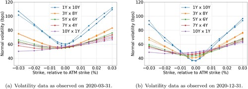
We consider data from two different market conditions. The first data-set is observed on 31 March 2020. This is during the peak of the Covid-19 pandemic, during which markets were stressed. The second data-set is observed nine months later, on 31 December 2020. On this date, markets were significantly less volatile. The solid lines in Figure 1 represent the implied volatility smiles extracted from the EUR 6M swaption market, for different co-terminal swaptions. The normal volatilities are displayed in basis-points as a function of the strike relative to the ATM strike in percentage points $(K=K_{\mathrm{A}\mathrm{T}\mathrm{M}}+x\mathrm{\%})$. We observe the following:

• In March 2020, the volatilities were relatively high, especially for short expiries.

• In December 2020 the ATM volatilities tend to increase as expiries increase, in March 2020 the ATM volatilities are rather invariant across expiries.

• In both periods, short expiries exhibit a strong smile, but little skew. For longer expiries the opposite is true.

• Relatively speaking, in March 2020 the skew is more profound, but in December 2020 the smile is more profound.

Figure 1. EUR 6M implied volatilities of co-terminal swaptions (solid) and Cheyette model calibration results (dashed) as a function of the strike, for different expiries and tenors. (a) Volatility data as observed on 2020-03-31 and (b) Volatility data as observed on 2020-12-31.

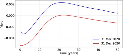
Yields as a function of maturity are for both periods displayed in Figure 2. The curves are nearly identical, apart from the fact that the yields in March were structurally higher. We observe a persistent difference of around 20 basis points.

Figure 2. EUR 6M yield curves as observed on 2020-03-31 and 2020-12-31.

4.2. Calibration Procedure

The calibration procedure is largely based on the approach described in Mikhailov and Nögel (2004). The model is calibrated to a set implied volatilities of 11 year co-terminal swaptions. That means the options used for calibration have different expiry times, but the underlying swaps will all mature in 11 years. The aim is to find the parameter set $\theta =\{\kappa ,\overline{v},ϵ,v_0,\rho \}$ that minimizes the objective function $L\left(\theta \right)$, given by (42) $L\left(\theta \right):=\sum _{(T,K)\in \mathcal{T}\times \mathcal{K}}{\left(V_{\mathrm{m}\mathrm{d}\mathrm{l}}\right(T,K;\theta )-V_{\mathrm{m}\mathrm{k}\mathrm{t}}(T,K;{\sigma }_{\mathrm{i}\mathrm{m}\mathrm{p}}\left)\phantom{|}\right)}^2$(42) with $\mathcal{T}=\left\{1\mathrm{Y},3\mathrm{Y},5\mathrm{Y},7\mathrm{Y}\right\}$ denoting the set of expiries and $\mathcal{K}=K_{\mathrm{A}\mathrm{T}\mathrm{M}}+\{-3\mathrm{\%},-1.5\mathrm{\%},-0.5\mathrm{\%},0\mathrm{\%},0.5\mathrm{\%},1.5\mathrm{\%},3\mathrm{\%}\}$ the set of strikes. We have experimented with different objective functions, including the squared distance between implied volatilities and swaption prices scaled by the reciprocal of Vega (data not shown). Each yielded a comparable fit to the market data. We selected the objective function given in (42(42) $L\left(\theta \right):=\sum _{(T,K)\in \mathcal{T}\times \mathcal{K}}{\left(V_{\mathrm{m}\mathrm{d}\mathrm{l}}\right(T,K;\theta )-V_{\mathrm{m}\mathrm{k}\mathrm{t}}(T,K;{\sigma }_{\mathrm{i}\mathrm{m}\mathrm{p}}\left)\phantom{|}\right)}^2$(42) ) for its compatibility with the analytical Vega calculations discussed in Section 3.4.2 and Appendix 6.

The market prices $V_{\mathrm{m}\mathrm{k}\mathrm{t}}$ are obtained by inserting the observed implied swaption volatilities into Bachelier's formula. The objective function is minimized using the differential evolution algorithm (Storn and Price 1997), which is a popular global optimization method. The reversion-speed parameter a of the short-rate process is fixed a priori, in correspondence with Casassus, Collin-Dufresne, and Goldstein (2005). The benchmark Hull–White model is calibrated to the same set of co-terminal swaptions, but only taking ATM strikes into account. Both models by construction allow for a perfect fit to the time-zero term-structure of interest rates observed in the market.

The calibrated parameters for the two different market states are shown in Table 1. The resulting implied model volatilities are displayed as dashed lines in Figure 1, next to the market volatilities. We observe a satisfactory fit to the market data, achieved with just a few degrees of freedom in the model parameters. The discrepancies tend to be the highest for the volatilities with the shortest maturity, where the smile is most profound and with the longest maturity, where the skew is most profound. The most accurate fit is achieved around the ATM strikes. The average relative error across strikes and maturities expressed as a percentage of the market volatility, is 3.3% for the March data and 2.4% for the December data.

Table 1. Calibrated model parameters.

	Cheyette						Hull–White
Parameter	a	κ	$\overline{v}\left({10}^{-5}\right)$	$ϵ\left({10}^{-2}\right)$	$v_0\left({10}^{-4}\right)$	ρ	a	$\sigma \left({10}^{-3}\right)$
2020-03-31	0.0825	1.7996	8.0732	3.6829	1.4301	0.1245	0.0825	8.6853
2020-12-31	0.0825	0.9952	6.4443	2.3687	0.3229	0.1714	0.0825	6.6896

5. Case Studies

In this section we present numerical results for three separate case studies: interest rate swaps, caps and vanilla swaptions. For each instrument we consider sensitivity profiles, future margin profiles and MVA charges. For each quantity we analyse the impact of including or excluding stochastic volatility for different moneyness levels of the instrument. The results are compared for two different market conditions and for backward- and forward-looking derivatives.

For the computation of the various risk metrics, we use a Monte Carlo simulation framework, such as for example presented in Zhu and Pykhtin (2007). Initial margin profiles are computed from the distribution of the future sensitivities of the derivative. The sensitivities are evaluated as described in Sections 3.3 and 3.4 and serve as input to compute forward SIMM margins. SIMM margins are calculated using the expressions and parameters provided in International Swaps and Derivatives Association, Inc (2020). Scenarios for the state-variable x are generated using an Euler discretization scheme. Scenarios for the volatility process v are generated using the QE scheme proposed in Andersen (2007). As we are dealing with volatility levels that are very close to zero, we implemented the refinement of the QE scheme as described in the appendix of Andersen (2007), to avoid a large number of zeros in the realizations of v. The scenarios are generated at equidistant time-points with monthly spacing. The sensitivity- and margin-profiles presented in the following sections are based on 100,000 paths. The MVA estimates for various levels of moneyness are based on 10,000 paths each and expressed in basis points relative to the notional. For the MVA computation, a constant funding spread of 100 basis points per annum is assumed (i.e., $\mathrm{F}\mathrm{S}\left(t\right)=0.01$).

5.1. Interest Rate Swaps

We start by analysing the interest rate swap. A distinction is made between the classic backward-looking swap written on the 6M LIBOR benchmark and the backward-looking swap written on RFR term rates. We consider a 1Yx10Y payer swap, exchanging annual fixed rate payments versus 6 months floating payments. To perform an intrinsic comparison between the forward- and backward-looking derivatives, experiments from the same period have been performed with the same model parameters and time-zero yield curve (see Section 4.1). In practice, the model calibration would be performed to RFR swaption data if RFR derivatives were considered. As RFR swaptions were not yet liquid on the selected dates, this is omitted for this study.

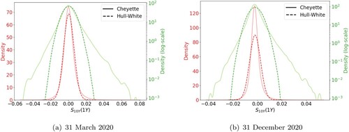
Figure 3 shows the risk-neutral probability densities for the 10Y swap rate, one year in the future. We consider the density under two market conditions on an linear scale and on a log scale. The densities on a linear scale reveal that the stochastic volatility exhibits higher peaks that are slightly shifted to the left. In March 2020 the shift is most profound, corresponding to the stronger skew. In December 2020 the peak is more profound corresponding to the stronger smile. Furthermore, the densities on a log scale indicate that the stochastic volatility induces fatter tails, assigning higher probability to tail events.

Figure 3. Risk-neutral densities of the 10Y swap rate after 1 year, displayed on a linear scale and a log scale. Plots are generated by calibrating the stochastic volatility Cheyette (solid) and the Hull–White (dashed) model to March 2020 (left) and December 2020 (right) data. (a) 31 March 2020 and (b) 31 December 2020.

The swap is a linear derivative, without optionality. In relation to SIMM it is therefore only exposed to Delta risk. Figure 4 presents the term-structure of the expected market value sensitivities of an ATM swap to the various SIMM interest rate risk factors. The sensitivities correspond to a basis point shift in the market rate with a standard SIMM tenor. The instrument is the most sensitive to changes in market rates with tenors corresponding to the swap maturity. Hence a sensitivity peaks at time t if the market rate tenor ${\tau }_k$ equals the time to maturity $T_M-t$, which can be explained by the $C_k$ coefficients. The sensitivity decays to zero as time approaches the maturity of the swap. The main difference between the forward- and backward-looking profile is the presence of the small negative sensitivities to the short-term market rates. A LIBOR swap will have negative peaks associated with rate tenors close to the next coupon fixing. These sensitivity peaks originate from the $\frac{P(t,T_i)}{P(T_{i-1},T_i)}$ term in (11(11) $V\left(t\right)=\{\begin{array}{ll}{\displaystyle \frac{P(t,T_i)}{P(T_{i-1},T_i)}-P(t,T_M)-\sum _{m=j}^{M^{\mathrm{\prime }}}{\tau }_j^{\mathrm{\prime }}KP(t,T_m^{\mathrm{\prime }})}& \mathrm{L}\mathrm{I}\mathrm{B}\mathrm{O}\mathrm{R}\mathrm{s}\mathrm{w}\mathrm{a}\mathrm{p}\\ {\displaystyle \frac{M_t}{M_{T_{i-1}}}-P(t,T_M)-\sum _{m=j}^{M^{\mathrm{\prime }}}{\tau }_j^{\mathrm{\prime }}KP(t,T_m^{\mathrm{\prime }})}& \mathrm{R}\mathrm{F}\mathrm{R}\mathrm{s}\mathrm{w}\mathrm{a}\mathrm{p}\end{array}$(11) ). The RFR coupons on the other hand gradually compound overnight during the accrual period, which is why the negative sensitivities are absent in subfigure (b). Furthermore, note that the difference between the Hull–White and Cheyette model is virtually zero. The dashed and solid lines in Figure 4 perfectly overlap, indicating a negligible impact of stochastic volatility on the Delta profiles.

Figure 4. Delta Sensitivities under Hull–White (dashed) and Cheyette (solid) for a 1Yx10Y forward-looking (left) and backward-looking (right) interest rate swap. The results for the ATM derivative on 31 March 2020 are shown. (a) Forward-looking swap and (b) Backward-looking swap.

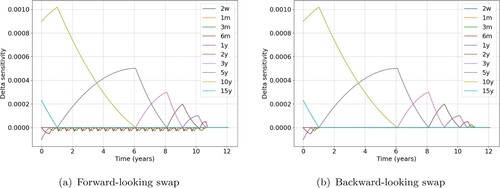
Figure 5 shows the Delta margin profile of the ATM swap for the two market conditions. We observe a ‘staircase’ profile for the forward-looking swap. After each coupon fixing, the instrument becomes less sensitive to the interest rate risk factors, which results in a discrete decay of the Delta-risk. The RFR term rates compound gradually, resulting in a continuous decay of the Delta-risk. The difference between the two periods can foremost be attributed to the expected yields, which were nearly identical in absolute terms. Hence the similarity between the March and December profile. We additionally investigated for different levels of moneyness and found that the margin profile hardly changes with different fixed rates.

Figure 5. Delta margin under Hull–White (blue) and Cheyette (red) for a 1Yx10Y forward-looking (dark) and backward-looking (light) interest rate swap. Results for 31 March 2020 (left) and 31 December 2020 (right) are shown. (a) ATM – March 2020 and (b) ATM – December 2020.

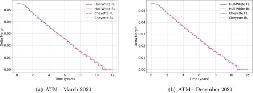
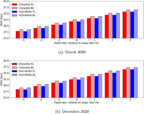
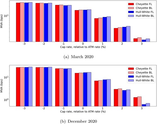
Figure 6 presents MVA charges related to the swap instrument for different levels of moneyness. MVA tends to increase as the fixed rate gets higher, which can be attributed to the valuation of the fixed flows. They yield a positive contribution to the Delta sensitivity and are scaled with the fixed rate K. We also note a difference of roughly one basis point between the charges for forward- and backward-looking swaps.

Figure 6. MVA charges under Hull–White and Cheyette for a 1Yx10Y forward-looking (dark) and backward-looking (light) interest rate swap. Results for 31 March 2020 (up) and 31 December 2020 (down) are shown for different levels of moneyness ($K=K_{\mathrm{A}\mathrm{T}\mathrm{M}}+x\mathrm{\%}$). (a) March 2020 and (b) December 2020.

5.2. Interest Rate Caps

Secondly we analyse a 1Yx10Y interest rate cap, with equidistant tenor structure of 6 months. Again a distinction is made between a cap written on the LIBOR and on the RFR benchmark. Experiments from the same period are performed with the same model parameters.

By the nature of a cap contract, it is exposed to Delta-, Curvature- and Vega-risk. As the Delta-risk is dominant in the IM valuation of a cap, we restrict the analysis to Delta margin and Delta implied MVA. Figure 7 presents the term-structure of the expected Delta sensitivities of an OTM cap to the various SIMM interest rate risk factors. Similar to the swap case, the instrument is the most sensitive to changes in market rates with tenors corresponding to the final cap maturity. Hence a sensitivity peaks at time t if the market rate tenor ${\tau }_k$ equals the time to maturity $T_M-t$. These peaks decay to zero as time approaches the maturity of the cap. Note that in contrast to the swap case, here the sensitivities tend to be slightly negative before they start to peak. In the expression for a swap price, many terms related to the floating flows cancel due to a telescoping sum, reflecting the symmetry of each floating payment. Due to the nonlinearity of each caplet, this is not the case for a cap, which results in these additional non-zero Delta sensitivities. Comparing the forward- to the backward-looking contract we note for the latter the absence of the small negative peaks corresponding to the short-term market rates. A LIBOR caplet that expires at $T_{j-1}$, guarantees a payment of $\mathrm{C}\mathrm{F}={\tau }_j\left(L\right(T_{j-1},T_j)-K{)}^{+}$ at time $T_j$. If $T_{j-1}<t<T_j$, the risk-neutral value of this cashflow (i.e., $P(t,T_j)\cdot \mathrm{C}\mathrm{F}$) has a strictly negative Delta sensitivity to changes in the short-term market rates, hence resulting in the small negative peaks. The RFR caplets on the other hand do not expire until the end of the accrual period, when the payment is executed.

Figure 7. Delta sensitivities under Hull–White (dashed) and Cheyette (solid) for a 1Yx10Y forward-looking (left) and backward-looking (right) interest rate cap. The results for the OTM derivative ($K=K_{\mathrm{A}\mathrm{T}\mathrm{M}}+1.5\mathrm{\%}$) on 31 March 2020 are shown. (a) Forward-looking cap and (b) Backward-looking cap.

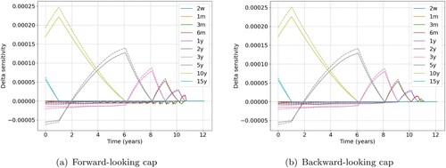
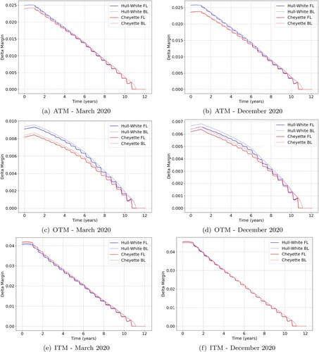
Figure 8 shows the Delta margin profiles of a cap for different levels of moneyness under the two market conditions. We again observe a ‘staircase’ profile for the forward-looking derivative versus a smooth profile for the backward-looking derivative. This reflects the fact that the Delta-risk of a LIBOR cap decays discretely with each instantaneous caplet fixing. The Delta-risk of an RFR cap however, decays continuously as the caplet fixings compounds gradually overnight during the accrual period. The impact of incorporating the volatility skew appears more pronounced for the cap compared to the swap. The Delta margin for ATM and OTM trades is tyically distinctively higher if modelled with a constant volatility. Analogously to the Black-Scholes model, the Delta can be thought of as the T-forward probability of the event that a caplet expires in-the-money. The peak of the Cheyette term rate density is shifted to the left, which explains the higher Delta-risks for the Hull–White model. The effect is most pronounced in March 2020, as this period exhibited the strongest skew. Only for far out-of-the-money trades, the fat tail property of the Cheyette model is dominant to the shifted peak, leading to higher Delta-risks with stochastic volatility.

Figure 8. Delta margin under Hull–White and Cheyette for a 1Yx10Y forward-looking (dark) and backward-looking (light) interest rate cap. Results for 31 March 2020 (left) and 31 December 2020 (right) are shown for three different moneyness levels, namely ATM, OTM ($K=K_{\mathrm{A}\mathrm{T}\mathrm{M}}+1.5\mathrm{\%}$) and ITM ($K=K_{\mathrm{A}\mathrm{T}\mathrm{M}}-1.5\mathrm{\%}$). (a) ATM – March 2020. (b) ATM – December 2020. (c) OTM – March 2020. (d) OTM – December 2020. (e) ITM – March 2020 and (f) ITM – December 2020.

The observations above are confirmed in Figure 9, which displays MVA charges associated to the Delta margin for different levels of moneyness. We note that MVA charges are mostly higher if modelled with constant volatility. The relative difference is at most around 10% for a moderately OTM cap rate. Only for $K=K_{\mathrm{A}\mathrm{T}\mathrm{M}}+3\mathrm{\%}$ (and above) we see the difference reversed. The MVA charge for a backward-looking cap is structurally higher than the forward-looking case, but this difference is only in the order of half a basis point.

Figure 9. MVA charges associated with Delta margin under Hull–White and Cheyette for a 1Yx10Y forward-looking (dark) and backward-looking (light) interest rate cap. Results for 31 March 2020 (up) and 31 December 2020 (down) are shown for different levels of moneyness ($K=K_{\mathrm{A}\mathrm{T}\mathrm{M}}+x\mathrm{\%}$). (a) March 2020 and (b) December 2020.

5.3. Swaptions

Lastly we analyse a 1Yx10Y payer swaption. The option is written on a fixed-floating payer swap, exchanging annual fixed rate payments versus 6 months floating payments. We assume the contract to be cash-settled, which means it terminates upon the option's expiry. The valuation of a forward-looking swaption is equivalent to that of a backward-looking one. As we use the same model parameters for the LIBOR and the RFR curve, we will not distinguish between the two derivative types. To value the swaption at some future simulation date t>0, we set $\overline{t}=t$ and let ${\tilde{S}}_t=S_t$, ${\tilde{v}}_t=v_t$. Then we proceed by valuing the contract based on the parameter-freezing approach as described in Section 3.2.

For a complete analysis we consider Delta-, Curvature- and Vega-risk for the swaption instrument. To obtain the various margin profiles we modelled both forward Delta and forward Vega sensitivities. The Vegas are evaluated by the approximation method described in Section 3.4.1. Figure 10 presents the term-structures of the expected swaption sensitivities, with the Deltas on the left and Vegas on the right. The instrument's sensitivity to changes in market rates is maximal for tenors corresponding to the maturity of the underlying swap. Hence a Delta sensitivity peaks at time t if the market rate tenor ${\tau }_k$ equals the time to the swap maturity $T_M-t$. Simultaneously the instrument has a negative sensitivity to changes in market rates with tenors corresponding to the expiry of the option. The Vega sensitivities are strictly positive and bucketed according to the time to expiry. The presented term-structures correspond to an ATM trade, corresponding to the March 2020 data.

Figure 10. Delta (left) and Vega (right) sensitivities under Hull–White (dashed) and Cheyette (solid) for a 1Yx10Y swaption. The results for the ATM derivative on 31 March 2020 are shown. (a) Delta sensitivities and (b) Vega sensitivities.

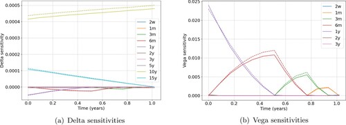
Figure 11 shows the swaption Delta margin profiles on the left, Curvature margin profiles in the middle and Vega margin profiles on the right, for different levels of moneyness. Results for the different market conditions are displayed in the same graph, with solid lines corresponding to March 2020 and dashed lines corresponding to December 2020. Delta and Curvature profiles show to be fairly persistent over time, whereas Vega margins show a smooth decay as it scales with the time to maturity of the option. Striking is that the Delta margin only exhibits a large difference between the two models for OTM trades. The Curvature and Vega margins exhibit large differences for both OTM and ITM trades. These results can be explained by an analogy to the Bachelier (or even Black-Scholes) model. The Delta is more or less proportional to the cumulative probability that the option expires in-the-money. Gamma and Vega on the other hand are more or less proportional to the probability density of the swap rate evaluated at the strike. Therefore the fat tail property of the Cheyette model has a large relative impact on the Delta if the strike is high and on the Gamma and Vega if the strike is either low or high. The relative differences for these levels of moneyness show to be in the order of a factor 10. We also note that for these trades the margins were significantly higher in March 2020, which can be attributed to the fatter tails of the swap rate distribution corresponding to that time.

Figure 11. Delta (left), Curvature (middle) and Vega (right) margin under Hull–White and Cheyette for a 1Yx10Y swaption. Results for 31 March 2020 (solid) and 31 December 2020 (dashed) are shown for three different moneyness levels, namely ATM, OTM ($K=K_{\mathrm{A}\mathrm{T}\mathrm{M}}+1.5\mathrm{\%}$) and ITM ($K=K_{\mathrm{A}\mathrm{T}\mathrm{M}}-1.5\mathrm{\%}$). (a) Delta margin – ATM. (b) Curvature margin – ATM. (c) Vega margin – ATM. (d) Delta margin – OTM. (e) Curvature margin – OTM. (f) Vega margin – OTM. (g) Delta margin – ITM. (h) Curvature margin – ITM and (i) Vega margin – ITM.

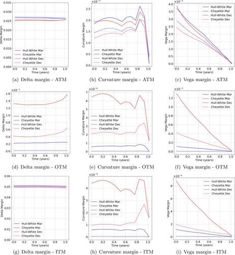
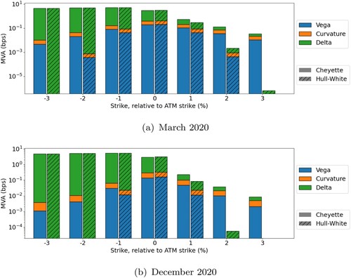
Figure 12 presents MVA charges, which are obtained by aggregating Delta-, Curvature- and Vega margins for different levels of moneyness. Carefully note that the charts are displayed on a log-scale. The contribution of the Delta-risk is dominant for most contracts. The contributions of Vega- and Curvature-risk are in the same order of magnitude, but typically several orders of magnitude smaller than Delta. We therefore note that the discrepancies of Curvature- and Vega Margin for ITM trades is of minor impact on the total MVA charge. Incorporation of the volatility skew does impact the MVA for OTM trades. For $K=K_{\mathrm{A}\mathrm{T}\mathrm{M}}+1\mathrm{\%}$, the MVA is already approximately two times higher for the stochastic volatility model. This relative difference only grows as the strike further increases, although the absolute MVA value sharply decreases with the strike. The impact is a result from the fat tail property of the swap rate distribution under the Cheyette model. We performed experiments for swaptions with longer expiries and noted that the impact of a stochastic volatility component decreases as the time to expiry grows. This also explains the difference in results between the cap and the swaption. A swaption expires instantly at the first fixing date of the swap, yielding a small probability that the option expires in-the-money. Therefore the impact of the fat tail property is dominant over the shifted peak of the risk factor density. The caplets that constitute a cap however have increasingly longer expiries, yielding higher and higher probabilities that such a caplet will expire in-the-money. Therefore, for most caplets the impact of the shifted peak is dominant over the fat tail property, yielding higher Delta margin with a constant volatility model. Overall the results suggest that a constant volatility model cannot capture the smile effects that influence MVA modelling, particularly for OTM swaptions.

Figure 12. MVA charges under Hull–White (striped) and Cheyette (non-striped) for a 1Yx10Y swaption. Results for 31 March 2020 (up) and 31 December 2020 (down) are shown for different levels of moneyness ($K=K_{\mathrm{A}\mathrm{T}\mathrm{M}}+x\mathrm{\%}$). (a) March 2020 and (b) December 2020.

6. Conclusion

In this research we studied the impact of a stochastic volatility on the computation of future initial margin and MVA for frequently traded interest rate derivatives. This impact is analysed by considering a Markovian short-rate model of Cheyette type, which is extended with a stochastic volatility component. The popular Hull–White model with constant volatility served as a benchmark. To perform a representative study, the models are calibrated to real market-data extracted under different market conditions. We considered case studies including interest rate swaps, caps and vanilla swaptions. The risk-metrics related to these derivatives are generated with a Monte Carlo simulation framework, where prices and sensitivities are obtained using Fourier transform techniques. The routines have been adapted to accommodate negative rates and the recent RFR benchmark, which has been selected to replace LIBOR. The expressions derived in this study are applied to model future ISDA SIMM quantities, but could also be used in broader risk management applications.

Linear contracts, such as the interest rate swap are only exposed to Delta-risk. We found that the margin profiles under the Cheyette and Hull–White are practically indistinguishable. A more significant impact is observed for nonlinear instruments. A striking result is that the Delta-risk modelled with a constant volatility turned out higher in most cases. This can be attributed to the shifted term rate distribution as a result from the calibration to the volatility smiles. Therefore, the effect is most distinct if implied volatilities are substantially skewed. Additionally, the transition from LIBOR to the overnight compounding RFR has transformed the ‘staircase’ margin profiles of both swaps and caps into a smoothly decaying profiles. By the backward-looking nature of the new term rates, cashflows remain sensitive to market changes until the end of the accrual period, yielding a persistently higher MVA. The most profound results were found for swaption contracts, for which Delta-, Curvature- and Vega-risk have been analysed. The latter two are substantially higher with stochastic volatility for both ITM and OTM trades. The Delta-risk is higher only for the OTM trades. As the Delta margin contribution to IM and MVA is dominant, only the OTM swaptions persist to be significantly affected in terms of MVA charges. We attribute this to the fat tails of the swap rate distribution under the Cheyette model. For the same reason the effect is weakened if the time to expiry is longer. With more time to expiry, the event of expiring in-the-money becomes less and less a ‘tail-event’.

Concluding, we have confirmed that stochastic volatility modelling for interest rate derivatives can have significant implications to IM and MVA valuation. It is well-known from the literature (see e.g., Collin-Dufresne and Goldstein 2002; Wu and Zhang 2006; Lorig and Suaysom 2022) that constant volatility models under- or overestimate the value of OTM, nonlinear derivatives. The same holds for risk metrics such as CVA and PFE, which depend on simulated future values of a derivative (see e.g., De Graaf et al. 2014; Simaitis et al. 2016). In this work we have shown that this effect extends to SIMM-IM and MVA, in particular for far out-of-the-money options. For a financial institution that has a uniform representation of moneyness levels in its portfolios, this may not be of direct concern. The IM volume for far out-of-the-money derivatives is relatively low, limiting the absolute material impact of an under- or overestimation. However, a substantial impact should be expected if OTM derivatives dominate the portfolio, for example after a sudden drop or sharp increase in the underlying market rates. In that case, a constant volatility model could significantly misprice future IM and its funding costs, which may have severe consequences in terms of risk management.

We have shown that extending a Cheyette short-rate model with a stochastic volatility component allows for a satisfactory fit to the market smiles, while remaining computationally tractable in a small number of state-variables and model parameters. Fourier transform techniques allow us to perform semi-closed form pricing and sensitivity calculation for common derivatives such as caps and swaptions. On top of that, the model and valuation routines have proven to be very suitable to accommodate the new set-in-arrears term rates.

Disclosure statement

The opinions expressed in this work are solely those of the authors and do not represent in any way those of their current and past employers. No potential conflict of interest was reported by the authors.

Additional information

Funding

This project has received funding from the NWO under the Industrial Doctorates grant.

Appendices

Appendix 1.

Proof of Proposition 3.1

Proof.

Consider the process $X\left(t\right)={\mathrm{e}}^{-{\int }_0^t{r}_u\mathrm{d}u}\exp \left\{C\right(t)+D(t)v_t+\omega \log P(t,T_{j-1})+(1-\omega )\log P(t,T_j\left)\right\}$ If $X\left(t\right)$ is a $\mathbb{Q}$-martingale, it follows that $\begin{array}{rl}\psi (\omega ,t)& ={\mathrm{e}}^{{\int }_0^t{r}_u\mathrm{d}u}{\mathbb{E}}^{\mathbb{Q}}\left[X\right(T_j\left)|{\mathcal{F}}_t\right]\\ & ={\mathrm{e}}^{{\int }_0^t{r}_u\mathrm{d}u}X\left(t\right)\\ & =\exp \left\{C\right(t)+D(t)v_t+\omega \log P(t,T_{j-1})+(1-\omega )\log P(t,T_j\left)\right\}\end{array}$ Now consider the process $y_i\left(t\right):=\log \left({\mathrm{e}}^{-{\int }_0^{t}r\left(s\right)ds}P\right(t,T_i\left)\right)$, which by Itô's lemma satisfies the SDE $d{y}_i\left(t\right)=-\sqrt{v_t}B(t,T_i){\mathbb{1}}_{\{t\le T_i\}}\mathrm{d}{W}_t-\frac{1}{2}{v}_t{B}^2(t,T_i){\mathbb{1}}_{\{t\le T_i\}}\mathrm{d}t$ To show that $X\left(t\right)$ is a martingale, note that it can be rewritten as $X\left(t\right)=\exp \left\{C\right(t)+D(t)v_t+\omega y_{j-1}(t)+(1-\omega \left)y_j\right(t\left)\right\}$ For ease of notation, denote $\overline{B}(t,T):=B(t,T){\mathbb{1}}_{\{t\le T\}}$. Applying Itô's lemma, yields the following dynamics $\begin{array}{rl}\frac{\mathrm{d}X\left(t\right)}{X\left(t\right)}& =(\dots )\mathrm{d}{W}_t+(\dots )\mathrm{d}{Z}_t+\left(\phantom{|}{C}^{\mathrm{\prime }}\right(t)+D(t\left)\kappa \overline{v}\right)\mathrm{d}t\\ & +\left(\phantom{|}{D}^{\mathrm{\prime }}\right(t)+\frac{1}{2}{ϵ}^2{D}^2(t)-(\kappa +ϵ\rho \omega \overline{B}(t,T_{j-1})+ϵ\rho (1-\omega \left)\overline{B}\right(t,T_j\left)\right)D(t)\\ & \phantom{|}-\frac{1}{2}\omega (1-\omega ){\left(\overline{B}\right(t,T_{j-1})-\overline{B}(t,T_j\left)\right)}^2)v_t\mathrm{d}t\end{array}$ It follows that $X\left(t\right)$ is $\mathbb{Q}$-martingale if $C(\cdot ),D(\cdot )$ satisfy the given ODEs.

Appendix 2.

Proof of Proposition 3.2

Proof.

To change the measure from $\mathbb{Q}$ to ${\mathbb{Q}}^{0,M}$, we consider the Radon–Nikodym derivative given by Geman, El Karoui, and Rochet (1995): $z_t:=\frac{\mathrm{d}\mathbb{Q}}{\mathrm{d}{\mathbb{Q}}^{A_{0,M}}}\left(t\right)=\frac{A_{0,M}\left(t\right)}{A_{0,M}\left(0\right)}\frac{M_0}{M_t}$ where $M_t$ denotes the money-market account and $A_{0,M}\left(t\right):=\sum _{m=1}^{M^{\mathrm{\prime }}}{\tau }_m^{\mathrm{\prime }}P(t,T_m^{\mathrm{\prime }})$ the annuity. To work out the differential of z, first note that $\mathrm{d}{A}_{0,M}\left(t\right)=r_t{A}_{0,M}\left(t\right)\mathrm{d}t-\sum _{m=1}^{M^{\mathrm{\prime }}}{\tau }_m^{\mathrm{\prime }}P(t,T_m^{\mathrm{\prime }})B(t,T_m^{\mathrm{\prime }})\sqrt{v_t}\mathrm{d}{W}_t$ and $d\left(\frac{1}{M_t}\right)=-\frac{r_t}{M_t}\mathrm{d}t$ Therefore, it follows by Itô's product rule that $\begin{array}{rl}d{z}_t& =\frac{M_0}{A_{0,M}\left(0\right)}\left(A_{0,M}\right(t)d\left(\frac{1}{M_t}\right)+\frac{1}{M_t}\mathrm{d}{A}_{0,M}(t\left)\right)\\ & =\frac{M_0}{A_{0,M}\left(0\right)}(-A_{0,M}(t)\frac{r_t}{M_t}\mathrm{d}t+\frac{r_t}{M_t}{A}_{0,M}(t)\mathrm{d}t-\sum _{m=1}^{M^{\mathrm{\prime }}}{\tau }_m^{\mathrm{\prime }}\frac{P(t,T_m^{\mathrm{\prime }})}{M_t}B(t,T_m^{\mathrm{\prime }}\left)\sqrt{v_t}\mathrm{d}{W}_t\right)\\ & =-z_t\sum _{m=1}^{M^{\mathrm{\prime }}}{\tau }_m^{\mathrm{\prime }}\frac{P(t,T_m^{\mathrm{\prime }})}{A_{0,M}\left(t\right)}B(t,T_m^{\mathrm{\prime }})\sqrt{v_t}\mathrm{d}{W}_t\end{array}$ Now, define $\mathrm{\Theta }\left(t\right):=\sum _{m=1}^{M^{\mathrm{\prime }}}{\tau }_m^{\mathrm{\prime }}\frac{P(t,T_m^{\mathrm{\prime }})}{A_{0,M}\left(t\right)}B(t,T_m^{\mathrm{\prime }})\sqrt{v_t}$. Note that $0\le {\tau }_m^{\mathrm{\prime }}\frac{P(t,T_m^{\mathrm{\prime }})}{A_{0,M}\left(t\right)}\le 1$ and $0\le B(t,T_m^{\mathrm{\prime }})\le \frac{1}{a}$ for all $m\in \{1,\dots ,M^{\mathrm{\prime }}\}$. Therefore, by Shirakawa (2002), the process $z_t$ is a true martingale under $\mathbb{Q}$ and satisfies the Novikov condition. As a consequence of Itô's lemma, $z_t$ solves to $z_t=\exp \{-{\int }_0^t\mathrm{\Theta }(u)\mathrm{d}{W}_u-\frac{1}{2}{\int }_0^t{\mathrm{\Theta }}^2(u\left)\mathrm{d}u\right\}$ and Θ represents Girsanov's kernel for the Radon–Nikodym process z. It follows by Girsanov's theorem that, if we denote $X\left(t\right):={\int }_0^t\mathrm{\Theta }\left(u\right)\mathrm{d}{W}_u$, then $\begin{array}{rl}\mathrm{d}{W}_t& =\mathrm{d}{W}_t^{0,M}-d{〈X,W〉}_t\\ & =\mathrm{d}{W}_t^{0,M}-\mathrm{\Theta }\left(t\right)d{〈W,W〉}_t\\ & =\mathrm{d}{W}_t^{0,M}-\mathrm{\Theta }\left(t\right)\mathrm{d}t\end{array}\begin{array}{rl}\mathrm{d}{Z}_t& =\mathrm{d}{Z}_t^{0,M}-d{〈X,Z〉}_t\\ & =\mathrm{d}{Z}_t^{0,M}-\mathrm{\Theta }\left(t\right)d{〈W,Z〉}_t\\ & =\mathrm{d}{Z}_t^{0,M}-\rho \mathrm{\Theta }\left(t\right)\mathrm{d}t\end{array}$ The swap rate is a martingale under ${\mathbb{Q}}^{0,M}$ (Jamshidian 1997). Therefore the ${\mathbb{Q}}^{0,M}$ dynamics of $S_{0,M}$ in (29(29) $\begin{array}{rl}\mathrm{d}{S}_{0,M}\left(t\right)& =\sqrt{v_t}\sum _{m=0}^{M^{\mathrm{\prime }}}{\zeta }_m\left(t\right)B(t,T_m^{\mathrm{\prime }})\mathrm{d}{W}_t^{0,M}\end{array}$(29) ) follow directly from substituting $\mathrm{d}{W}_t$. The ${\mathbb{Q}}^{0,M}$ dynamics of v are obtained as $\begin{array}{rl}\mathrm{d}{v}_t& =\kappa (\overline{v}-v_t)\mathrm{d}t+ϵ\sqrt{v\left(t\right)}\mathrm{d}{Z}_t\\ & =\kappa (\overline{v}-v_t)\mathrm{d}t+ϵ\sqrt{v_t}(\mathrm{d}{Z}_t^{0,M}-\rho \mathrm{\Theta }(t\left)\mathrm{d}t\right)\\ & =\kappa (\overline{v}-\xi (t\left)v_t\right)\mathrm{d}t+ϵ\sqrt{v_t}\mathrm{d}{Z}_t^{0,M}\end{array}$ where we denoted $\xi \left(t\right):=1+\rho \frac{ϵ\mathrm{\Theta }\left(t\right)}{\kappa \sqrt{v_t}}=1+\rho \frac{ϵ}{\kappa }\sum _{m=1}^{M^{\mathrm{\prime }}}{\tau }_m^{\mathrm{\prime }}B(t,T_m^{\mathrm{\prime }}){\xi }_m\left(t\right)$

Appendix 3.

Proof of proposition 3.3

Proof.

Consider the process $X\left(t\right)=\exp \left\{C\right(t)+D(t)v_t+i\omega S_{0,M}(t\left)\right\}$ If $X\left(t\right)$ is a ${\mathbb{Q}}^{0,M}$-martingale, it follows that $\begin{array}{rl}\psi (\omega ,t)& ={\mathbb{E}}^{0,M}\left[X\right(T_0\left)|{\mathcal{F}}_t\right]\\ & =X\left(t\right)\\ & =\exp \left\{C\right(t)+D(t)v_t+i\omega S_{0,M}(t\left)\right\}\end{array}$ Assume that $S_{0,M}$ satisfies th system of SDEs given in (31(31) $\begin{array}{rl}\mathrm{d}{\tilde{S}}_{0,M}\left(t\right)& =\sqrt{{\tilde{v}}_t}\sum _{m=0}^{M^{\mathrm{\prime }}}{\tilde{\zeta }}_{m}B(t,T_m^{\mathrm{\prime }})\mathrm{d}{W}_t^{0,M}\end{array}$(31) )–(32(32) $\begin{array}{rl}\mathrm{d}{\tilde{v}}_t& =\kappa (\overline{v}-\tilde{\xi }(t\left){\tilde{v}}_t\right)\mathrm{d}t+ϵ\sqrt{{\tilde{v}}_t}\mathrm{d}{Z}_t^{0,M}\end{array}$(32) ). Applying Itô's lemma to $X\left(t\right)$, then yields the following dynamics $\begin{array}{rl}\frac{\mathrm{d}X\left(t\right)}{X\left(t\right)}& =(\dots )\mathrm{d}{W}_t^{0,M}+(\dots )\mathrm{d}{Z}_t^{0,M}+\left(\phantom{|}{C}^{\mathrm{\prime }}\right(t)+D(t\left)\kappa \overline{v}\right)\mathrm{d}t\\ & +\left(D^{\mathrm{\prime }}\right(t)+\frac{1}{2}{ϵ}^2{D}^2(t)+\left(\rho ϵ\theta \right(t)i\omega -\kappa \tilde{\xi }(t\left)\right)D(t)-\frac{1}{2}{\omega }^2{\theta }^2(t\left)\right)v_t\mathrm{d}t\end{array}$ It follows that $X\left(t\right)$ is ${\mathbb{Q}}^{0,M}$-martingale if $C(\cdot ),D(\cdot )$ satisfy the given ODEs.

Appendix 4.

Proof of proposition 3.4

Proof.

We apply the pathwise derivative method introduced in Glasserman (2004). Note that the process $y_t:=\frac{P(t,T_{j-1})}{P(t,T_j)}$ is a martingale under the $T_j$-forward measure ${\mathbb{Q}}^{T_j}$ and satisfies the SDE $\mathrm{d}{y}_t=y_t\left(B\right(t,T_j){\mathbb{1}}_{\{t\le T_j\}}-B(t,T_{j-1}\left){\mathbb{1}}_{\{t\le T_{j-1}\}}\right)\sqrt{v_t}\mathrm{d}{W}_t^{T_j}$ where $W^{T_j}$ is a ${\mathbb{Q}}^{T_j}$ Brownian motion. Let ${\sigma }_j\left(t\right):=B(t,T_j){\mathbb{1}}_{\{t\le T_j\}}\sqrt{v_t}$. It is easy to show that conditioned on ${\mathcal{F}}_t$ the SDE above solves to (A1) $P(T_j,T_{j-1})=\{\begin{array}{ll}{\displaystyle \frac{P(t,T_{j-1})}{P(t,T_j)}{\mathrm{e}}^{{\int }_t^{T_j}\left({\sigma }_j\right(u)-{\sigma }_{j-1}(u\left)\right)\mathrm{d}{W}_u^{T_j}-\frac{1}{2}{\int }_t^{T_j}{\left({\sigma }_j\right(u)-{\sigma }_{j-1}(u\left)\right)}^2\mathrm{d}u}}& \mathrm{i}\mathrm{f}t<T_{j-1}\\ {\displaystyle \frac{{\mathrm{e}}^{{\int }_{T_{j-1}}^t{r}_u\mathrm{d}u}}{P(t,T_j)}{\mathrm{e}}^{{\int }_t^{T_j}{\sigma }_j\left(u\right)\mathrm{d}{W}_u^{T_j}-\frac{1}{2}{\int }_t^{T_j}{\sigma }_j^2\left(u\right)\mathrm{d}u}}& \mathrm{i}\mathrm{f}{T}_{j-1}\le t\le T_j\end{array}$(A1) Using this expression for $P(T_j,T_{j-1})$ allows us to compute the time-t zero-rate sensitivity of $P(T_j,T_{j-1})$, which is given by (A2) $\frac{\mathrm{\partial }P(T_j,T_{j-1})}{\mathrm{\partial }{R}_0(t,{\tau }_k)}=\{\begin{array}{ll}\left(\phantom{|}{C}_k\right(T_{j-1}-t)-C_k(T_j-t\left)\right)P(T_j,T_{j-1})& \mathrm{i}\mathrm{f}t<T_{j-1}\\ -C_k(T_j-t)P(T_j,T_{j-1})& \mathrm{i}\mathrm{f}{T}_{j-1}\le t<T_j\\ 0& \mathrm{i}\mathrm{f}t>T_j\end{array}$(A2) with the coefficients $C_k(\cdot )$ from (37(37) $C_k\left(\tau \right)=\{\begin{array}{ll}{\displaystyle \tau \frac{{\tau }_{k-1}-\tau }{{\tau }_k-{\tau }_{k-1}}}& \mathrm{i}\mathrm{f}{\tau }_{k-1}<\tau \le {\tau }_k\\ {\displaystyle \tau \frac{\tau -{\tau }_{k+1}}{{\tau }_{k+1}-{\tau }_k}}& \mathrm{i}\mathrm{f}{\tau }_k<\tau \le {\tau }_{k+1}\\ 0& \mathrm{o}\mathrm{t}\mathrm{h}\mathrm{e}\mathrm{r}\mathrm{w}\mathrm{i}\mathrm{s}\mathrm{e}\end{array}$(37) ). We proceed by computing the sensitivity of the conditional expectation $H(t,K_j):={\mathbb{E}}^{T_j}\left[\right(P(T_j,T_{j-1})-K_j{)}^{+}|{\mathcal{F}}_t]$ appearing in (18(18) $\begin{array}{rl}& =P(t,T_j){\mathbb{E}}^{T_j}\left[{\left(P\right(T_j,T_{j-1})-K_j)}^{+}|{\mathcal{F}}_t\right]\end{array}$(18) ). Application of the pathwise derivative method of Glasserman (2004) lets us take the derivative operator inside the expectation. It follows $\begin{array}{rl}\frac{\mathrm{\partial }H(t,K_j)}{\mathrm{\partial }{R}_0(t,{\tau }_k)}& ={\mathbb{E}}^{T_j}\left[\frac{\mathrm{\partial }}{\mathrm{\partial }{R}_0(t,{\tau }_k)}{\left(P\right(T_j,T_{j-1})-K)}^{+}|{\mathcal{F}}_t\right]\\ & ={\mathbb{E}}^{T_j}\left[\frac{\mathrm{\partial }{\left(P\right(T_j,T_{j-1})-K_j)}^{+}}{\mathrm{\partial }P(T_j,T_{j-1})}\frac{\mathrm{\partial }P(T_j,T_{j-1})}{\mathrm{\partial }{R}_0(t,{\tau }_k)}|{\mathcal{F}}_t\right]\\ & =\left(\phantom{|}{C}_k\right(T_{j-1}-t){\mathbb{1}}_{\{t\le T_{j-1}\}}-C_k(T_j-t\left){\mathbb{1}}_{\{t\le T_j\}}\right)\\ & \cdot {\mathbb{E}}^{T_j}\left[{\mathbb{1}}_{\{K_j<P(T_j,T_{j-1}\left)\right\}}P\right(T_j,T_{j-1}\left)|{\mathcal{F}}_t\right]\\ & =\left(\phantom{|}{C}_k\right(T_{j-1}-t){\mathbb{1}}_{\{t\le T_{j-1}\}}-C_k(T_j-t\left){\mathbb{1}}_{\{t\le T_j\}}\right){\mathrm{\Psi }}_1(t,K_j)\end{array}$ where in the third line we substituted (A2(A2) $\frac{\mathrm{\partial }P(T_j,T_{j-1})}{\mathrm{\partial }{R}_0(t,{\tau }_k)}=\{\begin{array}{ll}\left(\phantom{|}{C}_k\right(T_{j-1}-t)-C_k(T_j-t\left)\right)P(T_j,T_{j-1})& \mathrm{i}\mathrm{f}t<T_{j-1}\\ -C_k(T_j-t)P(T_j,T_{j-1})& \mathrm{i}\mathrm{f}{T}_{j-1}\le t<T_j\\ 0& \mathrm{i}\mathrm{f}t>T_j\end{array}$(A2) ). We finalize by an application of the product rule of differentiation to $V\left(t\right)$. Thus: $\begin{array}{rl}\frac{\mathrm{\partial }V\left(t\right)}{\mathrm{\partial }{R}_0(t,{\tau }_k)}& =H(t,K_j)\frac{\mathrm{\partial }P(t,T_j)}{\mathrm{\partial }{R}_0(t,{\tau }_k)}+P(t,T_j)\frac{\mathrm{\partial }H(t,K_j)}{\mathrm{\partial }{R}_0(t,{\tau }_k)}\\ & =\left(\phantom{|}{\mathrm{\Psi }}_1\right(t,K_j)-K_j{\mathrm{\Psi }}_0(t,K_j\left)\right)C_k(T_j-t){\mathbb{1}}_{\{t\le T_j\}}P(t,T_j)\\ & +P(t,T_j)\left(\phantom{|}{C}_k\right(T_{j-1}-t){\mathbb{1}}_{\{t\le T_{j-1}\}}-C_k(T_j-t\left){\mathbb{1}}_{\{t\le T_j\}}\right){\mathrm{\Psi }}_1(t,K_j)\\ & ={\mathbb{1}}_{\{t\le T_{j-1}\}}{C}_k(T_{j-1}-t){\mathrm{\Psi }}_1(t,K_j)-{\mathbb{1}}_{\{t\le T_j\}}{C}_k(T_j-t)K_j{\mathrm{\Psi }}_0(t,K_j)\end{array}$ This concludes the proof.

Appendix 5.

Proof of proposition 3.5

Proof.

We again apply the pathwise derivative method introduced in Glasserman (2004). It is assumed that the swap rate follows an arithmetic Brownian motion with adapted volatility ${\sigma }_S(\cdot )$. That means that conditioned on ${\mathcal{F}}_t$, the process $S_{0,M}$ above solves to (A3) $S_{0,M}\left(T_0\right)=S_{0,M}\left(t\right)+{\int }_t^{T_0}{\sigma }_S\left(u\right)\mathrm{d}{W}_u^{0,M}$(A3) Using the expression in (A3(A3) $S_{0,M}\left(T_0\right)=S_{0,M}\left(t\right)+{\int }_t^{T_0}{\sigma }_S\left(u\right)\mathrm{d}{W}_u^{0,M}$(A3) ) allows us to compute the time-t zero-rate sensitivity of $S_{0,M}\left(T_0\right)$. Application of the chain rules yields (A4) $\begin{array}{rl}\frac{\mathrm{\partial }{S}_{0,M}\left(T_0\right)}{\mathrm{\partial }{R}_0(t,{\tau }_k)}& =\frac{\mathrm{\partial }{S}_{0,M}\left(T_0\right)}{\mathrm{\partial }{S}_{0,M}\left(t\right)}\frac{\mathrm{\partial }{S}_{0,M}\left(t\right)}{\mathrm{\partial }{R}_0(t,{\tau }_k)}=1\cdot \frac{\mathrm{\partial }}{\mathrm{\partial }{R}_0(t,{\tau }_k)}\left(\frac{P(t,T_0)-P(t,T_M)}{\sum _{m=1}^{M^{\mathrm{\prime }}}{\tau }_m^{\mathrm{\prime }}P(t,T_m^{\mathrm{\prime }})}\right)\end{array}$(A4) (A5) $\begin{array}{rl}& =\frac{C_k(T_0-t)P(t,T_0)-C_k(T_M-t)P(t,T_M)}{\sum _{m=1}^{M^{\mathrm{\prime }}}{\tau }_m^{\mathrm{\prime }}P(t,T_m^{\mathrm{\prime }})}\end{array}$(A5) (A6) $\begin{array}{rl}& -S_{0,M}\left(t\right)\frac{\sum _{m=1}^{M^{\mathrm{\prime }}}{\tau }_m^{\mathrm{\prime }}{C}_k(T_m^{\mathrm{\prime }}-t)P(t,T_m^{\mathrm{\prime }})}{\sum _{m=1}^{M^{\mathrm{\prime }}}{\tau }_m^{\mathrm{\prime }}P(t,T_m^{\mathrm{\prime }})}\end{array}$(A6) with the coefficients $C_k(\cdot )$ from (37(37) $C_k\left(\tau \right)=\{\begin{array}{ll}{\displaystyle \tau \frac{{\tau }_{k-1}-\tau }{{\tau }_k-{\tau }_{k-1}}}& \mathrm{i}\mathrm{f}{\tau }_{k-1}<\tau \le {\tau }_k\\ {\displaystyle \tau \frac{\tau -{\tau }_{k+1}}{{\tau }_{k+1}-{\tau }_k}}& \mathrm{i}\mathrm{f}{\tau }_k<\tau \le {\tau }_{k+1}\\ 0& \mathrm{o}\mathrm{t}\mathrm{h}\mathrm{e}\mathrm{r}\mathrm{w}\mathrm{i}\mathrm{s}\mathrm{e}\end{array}$(37) ). We proceed by computing the sensitivity of the conditional expectation $\mathrm{\Psi }(t,K):={\mathbb{E}}^{0,M}\left[\right(S_{0,M}\left(T_0\right)-K{)}^{+}|{\mathcal{F}}_t]$ appearing in (19(19) $V\left(t\right)=\sum _{m=1}^{M^{\mathrm{\prime }}}{\tau }_m^{\mathrm{\prime }}P(t,T_m^{\mathrm{\prime }}){\mathbb{E}}^{0,M}\left[{\left(S_{0,M}\right(T_0)-K)}^{+}|{\mathcal{F}}_t\right]$(19) ). Application of the pathwise derivative method of Glasserman (2004) lets us take the derivative operator inside the expectation. Let ${\mathrm{\Psi }}_0(t,K):={\mathbb{E}}^{0,M}\left[{\mathbb{1}}_{\left\{S_{0,M}\right(T_0)>K\}}|{\mathcal{F}}_t\right]$. It follows $\begin{array}{rl}\frac{\mathrm{\partial }\mathrm{\Psi }(t,K)}{\mathrm{\partial }{R}_0(t,{\tau }_k)}& ={\mathbb{E}}^{0,M}\left[\frac{\mathrm{\partial }}{\mathrm{\partial }{R}_0(t,{\tau }_k)}{\left(S_{0,M}\right(T_0)-K)}^{+}|{\mathcal{F}}_t\right]\\ & ={\mathbb{E}}^{0,M}\left[\frac{\mathrm{\partial }{\left(S_{0,M}\right(T_0)-K)}^{+}}{\mathrm{\partial }{S}_{0,M}\left(T_0\right)}\frac{\mathrm{\partial }{S}_{0,M}\left(T_0\right)}{\mathrm{\partial }{R}_0(t,{\tau }_k)}|{\mathcal{F}}_t\right]\\ & =\frac{C_k(T_0-t)P(t,T_0)-C_k(T_M-t)P(t,T_M)}{\sum _{m=1}^{M^{\mathrm{\prime }}}{\tau }_m^{\mathrm{\prime }}P(t,T_m^{\mathrm{\prime }})}{\mathrm{\Psi }}_0(t,K)\\ & -S_{0,M}\left(t\right)\frac{\sum _{m=1}^{M^{\mathrm{\prime }}}{\tau }_m^{\mathrm{\prime }}{C}_k(T_m^{\mathrm{\prime }}-t)P(t,T_m^{\mathrm{\prime }})}{\sum _{m=1}^{M^{\mathrm{\prime }}}{\tau }_m^{\mathrm{\prime }}P(t,T_m^{\mathrm{\prime }})}{\mathrm{\Psi }}_0(t,K)\end{array}$ where in the third line we substituted (A5(A5) $\begin{array}{rl}& =\frac{C_k(T_0-t)P(t,T_0)-C_k(T_M-t)P(t,T_M)}{\sum _{m=1}^{M^{\mathrm{\prime }}}{\tau }_m^{\mathrm{\prime }}P(t,T_m^{\mathrm{\prime }})}\end{array}$(A5) )–(A6(A6) $\begin{array}{rl}& -S_{0,M}\left(t\right)\frac{\sum _{m=1}^{M^{\mathrm{\prime }}}{\tau }_m^{\mathrm{\prime }}{C}_k(T_m^{\mathrm{\prime }}-t)P(t,T_m^{\mathrm{\prime }})}{\sum _{m=1}^{M^{\mathrm{\prime }}}{\tau }_m^{\mathrm{\prime }}P(t,T_m^{\mathrm{\prime }})}\end{array}$(A6) ). We finalize by an application of the product rule of differentiation to $V\left(t\right)$. Thus: $\begin{array}{rl}\frac{\mathrm{\partial }V\left(t\right)}{\mathrm{\partial }{R}_0(t,{\tau }_k)}& =\mathrm{\Psi }(t,K)\frac{\mathrm{\partial }\sum _{m=1}^{M^{\mathrm{\prime }}}{\tau }_m^{\mathrm{\prime }}P(t,T_m^{\mathrm{\prime }})}{\mathrm{\partial }{R}_0(t,{\tau }_k)}+\sum _{m=1}^{M^{\mathrm{\prime }}}{\tau }_m^{\mathrm{\prime }}P(t,T_m^{\mathrm{\prime }})\frac{\mathrm{\partial }\mathrm{\Psi }(t,K)}{\mathrm{\partial }{R}_0(t,{\tau }_k)}\\ & =\left(\phantom{|}{C}_k\right(T_0-t\left)P\right(t,T_0)-C_k(T_M-t\left)P\right(t,T_M\left)\right){\mathrm{\Psi }}_0(t,K)\\ & +\sum _{m=1}^{M^{\mathrm{\prime }}}{\tau }_m^{\mathrm{\prime }}{C}_k(T_m^{\mathrm{\prime }}-t)P(t,T_m)\left(\phantom{|}\mathrm{\Psi }\right(t,K)-S_{0,M}(t\left){\mathrm{\Psi }}_0\right(t,K\left)\right)\end{array}$ This concludes the proof.

Appendix 6.

Vega computation for general nonlinear instruments

Denote by θ the vector of model parameters, and denote by ${\sigma }_{\mathrm{i}\mathrm{m}\mathrm{p}}=({\sigma }_{2\mathrm{W}},\dots ,{\sigma }_{30\mathrm{Y}}{)}^{\mathrm{\top }}$ the vector of implied swaption volatilities. The model parameters are chosen such that the model output matches the (observed) implied volatilities as good as possible. In that sense, θ depends on the implied volatilities through the objective function L given in (42(42) $L\left(\theta \right):=\sum _{(T,K)\in \mathcal{T}\times \mathcal{K}}{\left(V_{\mathrm{m}\mathrm{d}\mathrm{l}}\right(T,K;\theta )-V_{\mathrm{m}\mathrm{k}\mathrm{t}}(T,K;{\sigma }_{\mathrm{i}\mathrm{m}\mathrm{p}}\left)\phantom{|}\right)}^2$(42) ), which is minimized during the calibration procedure. Assume that for the parameter set θ the objective function L is indeed minimized. Then according to the first-order optimality condition, the following relation is satisfied (Beinker and Schlenkrich 2017) $\frac{\mathrm{\partial }L(\theta ,{\sigma }_{\mathrm{i}\mathrm{m}\mathrm{p}})}{\mathrm{\partial }\theta }:={\left(\begin{array}{ccc}{\displaystyle \frac{\mathrm{\partial }L(\theta ,{\sigma }_{\mathrm{i}\mathrm{m}\mathrm{p}})}{\mathrm{\partial }{\theta }_1}}& \cdots & {\displaystyle \frac{\mathrm{\partial }L(\theta ,{\sigma }_{\mathrm{i}\mathrm{m}\mathrm{p}})}{\mathrm{\partial }{\theta }_d}}\end{array}\right)}^{\mathrm{\top }}=\overrightarrow{0}$ for our particular objective function, the derivative above is given by $\frac{\mathrm{\partial }L(\theta ,{\sigma }_{\mathrm{i}\mathrm{m}\mathrm{p}})}{\mathrm{\partial }{\theta }_j}=\sum _{(\tau ,K)\in \mathcal{T}\times \mathcal{K}}2\frac{\mathrm{\partial }{V}_{\mathrm{m}\mathrm{d}\mathrm{l}}(\tau ,K;\theta )}{\mathrm{\partial }{\theta }_j}\left(V_{\mathrm{m}\mathrm{d}\mathrm{l}}\right(\tau ,K;\theta )-V_{\mathrm{m}\mathrm{k}\mathrm{t}}(\tau ,K;{\sigma }_{\mathrm{i}\mathrm{m}\mathrm{p}}\left)\phantom{|}\right)$ where $V_{\mathrm{m}\mathrm{d}\mathrm{l}}$ denotes the model-implied swaption price and $V_{\mathrm{m}\mathrm{k}\mathrm{t}}$ the swaption price associated to the (observed) implied volatility. Now write $\lambda (\theta ,{\sigma }_{\mathrm{i}\mathrm{m}\mathrm{p}}):=\frac{\mathrm{\partial }L(\theta ,{\sigma }_{\mathrm{i}\mathrm{m}\mathrm{p}})}{\mathrm{\partial }\theta }$, then it follows by the implicit function theorem that $\frac{\mathrm{\partial }\theta }{\mathrm{\partial }{\sigma }_{\mathrm{i}\mathrm{m}\mathrm{p}}}=-\frac{\mathrm{\partial }\lambda }{\mathrm{\partial }{\sigma }_{\mathrm{i}\mathrm{m}\mathrm{p}}}(\frac{\mathrm{\partial }\lambda }{\mathrm{\partial }\theta }{)}^{-1}$. Now let $V(\cdot )$ (without mkt or mdl subscript) denote the risk-neutral value of the product under consideration. A subsequent application of the the multi-dimensional chain rule, yields the desired sensitivity vector: (A7) $\left(\begin{array}{c}{\displaystyle \frac{\mathrm{\partial }V}{\mathrm{\partial }{\sigma }_{2\mathrm{W}}}}\\ ⋮\\ {\displaystyle \frac{\mathrm{\partial }V}{\mathrm{\partial }{\sigma }_{30\mathrm{Y}}}}\end{array}\right)=-\left(\begin{array}{ccc}{\displaystyle \frac{{\mathrm{\partial }}^{2}L}{\mathrm{\partial }{\sigma }_{2\mathrm{W}}\mathrm{\partial }{\theta }_1}}& \cdots & {\displaystyle \frac{{\mathrm{\partial }}^{2}L}{\mathrm{\partial }{\sigma }_{2\mathrm{W}}\mathrm{\partial }{\theta }_d}}\\ ⋮& \ddots & ⋮\\ {\displaystyle \frac{{\mathrm{\partial }}^{2}L}{\mathrm{\partial }{\sigma }_{30\mathrm{Y}}\mathrm{\partial }{\theta }_1}}& \cdots & {\displaystyle \frac{{\mathrm{\partial }}^{2}L}{\mathrm{\partial }{\sigma }_{30\mathrm{Y}}\mathrm{\partial }{\theta }_d}}\end{array}\right){\left(\begin{array}{ccc}{\displaystyle \frac{{\mathrm{\partial }}^{2}L}{\mathrm{\partial }{\theta }_1^2}}& \cdots & {\displaystyle \frac{{\mathrm{\partial }}^{2}L}{\mathrm{\partial }{\theta }_1\mathrm{\partial }{\theta }_d}}\\ ⋮& \ddots & ⋮\\ {\displaystyle \frac{{\mathrm{\partial }}^{2}L}{\mathrm{\partial }{\theta }_d\mathrm{\partial }{\theta }_1}}& \cdots & {\displaystyle \frac{{\mathrm{\partial }}^{2}L}{\mathrm{\partial }{\theta }_d^2}}\end{array}\right)}^{-1}\left(\begin{array}{c}{\displaystyle \frac{\mathrm{\partial }V}{\mathrm{\partial }{\theta }_1}}\\ ⋮\\ {\displaystyle \frac{\mathrm{\partial }V}{\mathrm{\partial }{\theta }_d}}\end{array}\right)$(A7) An exact derivation of the matrix entries above is tedious and falls outside the scope of this paper.

References

- Andersen Leif B. G. 2007. “Efficient Simulation of the Heston Stochastic Volatility Model.” SSRN 946405.
- Andersen Leif, and Andreasen Jesper. 2000. “Volatility Skews and Extensions of the LIBOR Market Model.” Applied Mathematical Finance 7 (1): 1–32. doi:10.1080/135048600450275
- Andersen Leif B. G., and Brotherton-Ratcliffe Rupert. 2001. “Extended LIBOR market models with stochastic volatility.” SSRN 294853.
- Andersen Leif B. G., and Piterbarg Vladimir V.. 2010. Interest Rate Modeling, Volume II: Term Structure Models. London: Atlantic Financial Press.
- Antonov Alexandre, Issakov Serguei, and McClelland Andy. 2017. “Efficient SIMM-MVA Calculations for Callable Exotics.” SSRN 3040061.
- Bank for International Settlements. 2021. “OTC Derivatives Statistics.” Accessed October 08. http://stats.bis.org/statx/.
- Basel Committee on Banking Supervision. 2010. “Basel III: A Global Framework for More Resilient Banks and Banking System”.
- Beinker Mark, and Schlenkrich Sebastian. 2017. “Accurate Vega Calculation for Bermudan Swaptions.” In Novel Methods in Computational Finance, 65–82. Springer.
- Biagini Francesca, Gnoatto Alessandro, and Oliva Immacolata. 2019. “Pricing of Counterparty Risk and Funding With CSA Discounting, Portfolio Effects and Initial Margin.” arXiv preprint arXiv:1905.11328.
- Biagini Francesca, Gnoatto Alessandro, and Oliva Immacolata. 2021. “A Unified Approach to xVA With CSA Discounting and Initial Margin.” SSRN 3394928.
- Brigo Damiano, and Mercurio Fabio. 2006. Interest Rate Models-Theory and Practice: With Smile, Inflation and Credit. Vol. 2. Berlin: Springer.
- Burgard Christoph, and Kjaer Mats. 2013. “Funding Strategies, Funding Costs.” Risk (Concord, NH) 26 (12): 82.
- Carr Peter, and Madan Dilip. 1999. “Option Valuation Using the Fast Fourier Transform.” Journal of Computational Finance 2 (4): 61–73. doi:10.21314/JCF.1999.043
- Casassus Jaime, Collin-Dufresne Pierre, and Goldstein Bob. 2005. “Unspanned Stochastic Volatility and Fixed Income Derivatives Pricing.” Journal of Banking & Finance 29 (11): 2723–2749. doi:10.1016/j.jbankfin.2005.02.007
- Caspers Peter, and Lichters Roland. 2018. “Initial Margin Forecast-Bermudan Swaption Methodology and Case Study.” SSRN 3132008.
- Cheyette Oren. 2001. “Markov Representation of the Heath-Jarrow-Morton Model.” SSRN 6073.
- Collin-Dufresne Pierre, and Goldstein Robert S.. 2002. “Do Bonds Span the Fixed Income Markets? Theory and Evidence for Unspanned Stochastic Volatility.” The Journal of Finance 57 (4): 1685–1730. doi:10.1111/1540-6261.00475
- De Graaf Cornelis S. L., Feng Qian, Kandhai Drona, and Oosterlee Cornelis W.. 2014. “Efficient Computation of Exposure Profiles for Counterparty Credit Risk.” International Journal of Theoretical and Applied Finance 17 (04): Article ID 1450024. doi:10.1142/S0219024914500241
- Filipovic Damir. 2009. Term-Structure Models. A Graduate Course. Berlin: Springer.
- Fries Christian P. 2019. “Fast Stochastic Forward Sensitivities in Monte Carlo Simulations Using Stochastic Automatic Differentiation (with Applications to Initial Margin Valuation Adjustments).” Journal of Computational Finance 22 (4): 103–125. doi:10.21314/JCF.2018.359
- Garcia Trillos Camilo A., Henrard Marc, and Macrina Andrea. 2016. “Estimation of Future Initial Margins in a Multi-Curve Interest Rate Framework.” SSRN 2682727.
- Geman Helyette, El Karoui Nicole, and Rochet Jean-Charles. 1995. “Changes of Numeraire, Changes of Probability Measure and Option Pricing.” Journal of Applied Probability 32 (2): 443–458. doi:10.2307/3215299
- Glasserman Paul. 2004. Monte Carlo Methods in Financial Engineering. Vol. 53. New York: Springer.
- Green Andrew. 2015. XVA: Credit, Funding and Capital Valuation Adjustments. Chichester: John Wiley & Sons.
- Green Andrew David, and Kenyon Chris. 2015. “MVA: Initial Margin Valuation Adjustment by Replication and Regression.” SSRN 2432281.
- Gregory Jon. 2020. The XVA Challenge: Counterparty Risk, Funding, Collateral, Capital and Initial Margin. Chichester: John Wiley & Sons.
- Harrison J. Michael, and Pliska Stanley R.. 1981. “Martingales and Stochastic Integrals in the Theory of Continuous Trading.” Stochastic Processes and Their Applications 11 (3): 215–260. doi:10.1016/0304-4149(81)90026-0
- Hull John, and White Alan. 1990. “Pricing Interest-rate-derivative Securities.” The Review of Financial Studies 3 (4): 573–592. doi:10.1093/rfs/3.4.573
- International Swaps and Derivatives Association, Inc. 2016. “ISDA SIMM: From Principles to Model Specification”.
- International Swaps and Derivatives Association, Inc. 2020. “ISDA SIMM: Methodology, Version 2.3”.
- International Swaps and Derivatives Association, Inc. 2021. “ISDA Margin Survey Year-End 2020”.
- Jäckel Peter. 2017. “Implied Normal Volatility.” Wilmott 2017 (90): 54–57. doi:10.1002/wilm.2017.2017.issue-90
- Jamshidian Farshid. 1997. “LIBOR and Swap Market Models and Measures.” Finance and Stochastics 1 (4): 293–330. doi:10.1007/s007800050026
- Lakhany Asif, and Zhang Amber. 2021. “Efficient ISDA Initial Margin Calculations Using Least Squares Monte-Carlo.” arXiv preprint arXiv:2110.13296.
- Lee Roger W. 2004. “Option Pricing by Transform Methods: Extensions, Unification and Error Control.” Journal of Computational Finance 7 (3): 51–86. doi:10.21314/JCF.2004.121
- Lorig Matthew, and Suaysom Natchanon. 2022. “Options on Bonds: Implied Volatilities From Affine Short-rate Dynamics.” Annals of Finance 18 (2): 1–34.
- Lyashenko Andrei, and Mercurio Fabio. 2019. “Looking Forward to Backward-Looking Rates: A Modeling Framework for Term Rates Replacing LIBOR.” SSRN 3330240.
- Ma Xun, Spinner Sogee, Venditti Alex, Li Zhao, and Tang Strong. 2019. “Initial Margin Simulation with Deep Learning.” SSRN 3357626.
- McWalter Thomas, Kienitz Jörg, Nowaczyk Nikolai, Rudd Ralph, and Acar Sarp Kaya. 2018. “Dynamic Initial Margin Estimation Based on Quantiles of Johnson Distributions.” SSRN 3147811.
- Mercurio Fabio. 2018. “A Simple Multi-Curve Model for Pricing Sofr Futures and Other Derivatives.” SSRN 3225872.
- Mikhailov Sergei, and Nögel Ulrich. 2004. Heston's Stochastic Volatility Model: Implementation, Calibration and Some Extensions. Chichester: John Wiley and Sons.
- Munk Claus. 1999. “Stochastic Duration and Fast Coupon Bond Option Pricing in Multi-factor Models.” Review of Derivatives Research 3 (2): 157–181. doi:10.1023/A:1009654427422
- Musiela Marek, and Rutkowski Marek. 1997. Martingale Methods in Financial Modeling. 2nd ed. Berlin: Springer.
- Ritchken Peter, and Sankarasubramanian L.. 1995. “Volatility Structures of Forward Rates and the Dynamics of the Term Structure 1.” Mathematical Finance 5 (1): 55–72. doi:10.1111/mafi.1995.5.issue-1
- Schrager David F, and Pelsser Antoon A. J.. 2006. “Pricing Swaptions and Coupon Bond Options in Affine Term Structure Models.” Mathematical Finance 16 (4): 673–694. doi:10.1111/mafi.2006.16.issue-4
- Shirakawa Hiroshi. 2002. “Squared Bessel Processes and Their Applications to the Square Root Interest Rate Model.” Asia-Pacific Financial Markets 9 (3): 169–190. doi:10.1023/A:1024173313448
- Simaitis S., de Graaf C. S. L., Hari N., and Kandhai D.. 2016. “Smile and Default: The Role of Stochastic Volatility and Interest Rates in Counterparty Credit Risk.” Quant. Finance 16 (11): 1725–1740. doi:10.1080/14697688.2016.1176240
- Storn Rainer, and Price Kenneth. 1997. “Differential Evolution–a Simple and Efficient Heuristic for Global Optimization Over Continuous Spaces.” Journal of Global Optimization 11 (4): 341–359. doi:10.1023/A:1008202821328
- Trolle Anders B., and Schwartz Eduardo S.. 2009. “A General Stochastic Volatility Model for the Pricing of Interest Rate Derivatives.” The Review of Financial Studies 22 (5): 2007–2057. doi:10.1093/rfs/hhn040
- Vierkoetter Matthias. 2019. “The Impact of Initial Margin on Derivatives Pricing with an Application of Machine Learning.” SSRN 3427230.
- Wei Jason Z. 1997. “A Simple Approach to Bond Option Pricing.” Journal of Futures Markets: Futures, Options, and Other Derivative Products 17 (2): 131–160. doi:10.1002/(ISSN)1096-9934
- Wu Lixin, and Zhang Fan. 2006. “LIBOR Market Model with Stochastic Volatility.” Journal of Industrial & Management Optimization 2 (2): 199. doi:10.3934/jimo.2006.2.199
- Zeron Mariano, and Ruiz Ignacio. 2018. Dynamic Initial Margin via Chebyshev Spectral Decomposition. Technical Report. Working paper (24 August).
- Zhu Steven H., and Pykhtin Michael. 2007, July/August. “A Guide to Modeling Counterparty Credit Risk.” GARP Risk Review.