Optimal Execution: A Review

Abstract

This review article is intended to collect and summarize many of the results in the field of optimal execution over the last twenty years. In doing so, we describe the general workings of the limit order book so that the sources of costs and risks which need to be optimized are understood. The initial models considered propose simple dynamics for prices which allow easily computable strategies which maximize risk-adjusted profits. Subsequently, the review is divided into two major parts. The first explores several works which investigate how optimal liquidation strategies are modified to account for more complex dynamics, namely other stochastic or non-linear factors. The second presents optimal trading strategies when the agent utilizes benchmarks in addition to risk-adjusted wealth, or when she has objectives beyond optimal liquidation.

Keywords:

• Algorithmic trading
• price impact
• stochastic optimization

1. Introduction

In the last few decades, the actions taken by participants in financial markets have become increasingly based on quantitative analysis and algorithms rather than any human decision making process. The motivation for this shift comes from attempting to minimize costs associated with trading, or to minimize risks involved in holding financial assets, or both. Establishing a mathematical framework that models the setting of trading in a financial market allows one to quantify the trade-off between minimizing costs and minimizing risks, thereby tailoring a trading strategy to one's preferences optimally. In this review article, we provide an overview of many developments and results related to optimal execution of trades.

We begin with a description of the limit order book (LOB), and then proceed with a summary of some preliminary models in discrete time, in particular those of Bertsimas and Lo (1998) and R. Almgren and Chriss (2001). These pieces will provide a groundwork for the type of problems considered in this review, but most of the focus will be on analogous models and results in continuous time. After this groundwork is established, we review developments which take more realistic or generalized underlying dynamics, different or more general performance criteria, and other aspects of financial trading and optimization.

The primary mathematical tools that are used to solve many of the problems contained herein are the Dynamic Programming Principle (DPP) and the Hamilton–Jacobi–Bellman (HJB) equation, although sometimes other approaches such as variational techniques are necessary. The full solutions to optimizations are omitted, but the original sources of the results or standard references on stochastic optimal control should provide any details which are skipped (see for example Yong and Zhou 1999; Fleming and Soner 2006).

We focus on modelling and optimization results of a theoretical nature, but many of the primary sources that are cited contain empirical analysis to motivate modelling choices. Some of these motivational empirical results will be provided when warranted, but the discussion about these results and their interpretation will be limited.

2. The Limit Order Book

This section describes the general mechanisms of the LOB. An understanding of how transactions take place within LOBs motivates some of the modelling choices in the next section. Many of these modelling choices may still be appropriate in other market settings that do not employ a LOB, nevertheless a specific context may help with interpretation of results that we present later.

Most electronic exchanges allow participants to submit several different types of orders, but these can be categorized broadly as either passive limit orders (LOs) or aggressive market orders (MOs), so for clarity we describe a simplified form of LOB mechanisms containing only the most basic of these two types of orders.

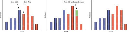
LOs consist of a price, a volume, and an indicator to either buy or sell the asset. After an LO is submitted, it sits in the LOB until it is either cancelled or filled against an MO at a later time. The cancellation or filling of an LO can be either full or partial, meaning either the entire volume of the order is removed from the LOB or some amount of the original volume remains in the LOB. If a subsequent LO is placed with the same price, then both of these orders will exist simultaneously in the LOB at this price, and the order of execution of the orders depends on the matching rules of the exchange. The matching rules we describe below correspond to a price-time priority of orders, meaning the LOs form a queue at each price and the LOs to be filled are determined according to their position in this queue, known as the First In First Out (FIFO) rule.¹ When several LOs of different types (buys and sells) are sitting in the LOB, there are two price levels which correspond to the highest price across all buy LOs and the lowest price across all sell LOs, referred to as the best bid and best ask, respectively. The average of the best bid and best ask is referred to as the midprice of the asset. Figure 1 shows a graphical representation of the state of the LOB at a single point in time, followed by the state of the LOB after a single LO is placed.

Figure 1. Blue bars represent buy LOs, red bars represent sell LOs. Left panel: the highest price of all buy LOs and the lowest price of all sell LOs are the best bid and ask, respectively. Middle panel: a new LO is placed at a price where orders already exist at the back of the queue. Right panel: the volume at this price is increased. Analogous changes would result from an order cancellation, and thus the state of the LOB may change through time, even if no trades are taking place.

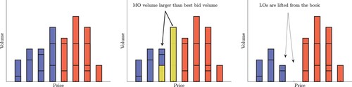
An MO consists of a volume and indicator to either buy or sell the asset. When an MO is submitted it is matched against resting LOs of the opposite buy/sell type, and the price of the transaction is determined by the price level of all filled LOs up to the volume specified by the MO. In Figure 2 we show a graphical representation of an MO filling several LOs to illustrate how the volume of the MO and the volumes and prices of the LOs determine the overall transaction price of this trade.

Figure 2. Left panel: the LOB immediately before an MO is submitted. Middle panel: a sell MO is submitted with volume greater than that of the best bid, so it must ‘walk the book’ into the next best price. Right panel: the MO has filled LOs in the book, so there is now less volume available at the two relevant prices.

With this structure of the LOB in mind, it is clear that the midprice of the asset may change through time as LOs are placed and cancelled near the best bid and ask. Additionally, the effect that MOs have on prices can be interpreted in multiple ways. We generally divide the impact of MOs into temporary and permanent, although they are not fully distinct and there may be other impact phenomena which don't fall into either category. Temporary price impact refers to the relationship between the volume of the MO and the average execution price of the trade. For larger MOs, multiple LOs at different levels are executed, thus the average price of the trade is a function of volume. Permanent price impact refers to the relationship between the volume of the MO and the midprice process at future times after the execution. For larger MOs, more LOs are removed from the LOB resulting in a greater change of the midprice which will persist into the future, affecting the price of subsequent trades.

The LOB structure discussed above is an idealization of real markets where there are several types of orders that can be submitted. Usually, order types can be loosely grouped by whether they add or remove liquidity from the market, and we think of them as LOs or MOs, respectively, in our idealized framework. These other order types include stop-loss, stop-limit, immediate-or-cancel, fill-or-kill, and all-or-none.

For extensive analysis on LOB dynamics, including and beyond price-impact effects, see Biais, Hillion, and Spatt (1995), Ranaldo (2004), R. Almgren et al. (2005), Cont (2011), Cont, Kukanov, and Stoikov (2014), Cartea, Jaimungal, and Penalva (2015), Lehalle and Mounjid (2017), Bechler and Ludkovski (2017), Cartea, Donnelly, and Jaimungal (2018a), and Sirignano (2019). For more in depth outline of the operation of LOBs in financial markets and of advanced order types, see Cartea, Jaimungal, and Penalva (2015) and Guéant (2016).

3. Modeling Trades, Price Impact, and Objectives

3.1. Discrete-Time Model

The discrete time model that we present here is adapted from the models first established in Bertsimas and Lo (1998) and R. Almgren and Chriss (2001), and which have consistently formed the basis for most models in discrete time optimal execution since then. While Bertsimas and Lo (1998) takes into account additional considerations such as informed price changes and more realistic dynamics, the initial model they propose to get intuition about optimal execution is equivalent to what we give below.

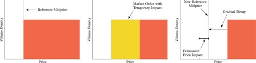
We make a conceptual change to the description of the LOB in the previous section to motivate many of the assumptions made in this model. The main change we make is that we consider the LOB to be based on a continuum of prices rather than a discrete set, and the LOs form a volume density, rather than a collection of individual queues at each price. Thus, our graphical representation including the arrival of an MO changes to that of Figure 3.

Figure 3. Left panel: the LOB as volume density. Middle panel: a sell MO is submitted with volume equal to the area of the yellow region. Right panel: the MO has filled LOs in the book, and both buy and sell LOs are shortly thereafter placed to establish a new impacted midprice.

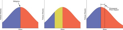
Note that in the right-hand panel of Figure 3, the new midprice is located between (not necessarily at the midpoint) the old midprice and the lowest executed price of the MO from the middle panel. We assume that immediately after the MO, there is a flurry of activity in the LOB which includes many new LO placements to establish this new midprice. This activity could potentially also include LO cancellations resulting in a new midprice beyond the lowest executed price. In addition, there is no gap left in the LOB and indeed the overall shape is merely a translation of the original shape. This will be reflected in the model below through the fact that our impact functions depend only on the size of the MO.

We work on a finite time horizon equal to N and index time by $n\in \{0,\dots ,N\}$. Let $Q=\{Q_n{\}}_{n=0}^N$ be the agent's inventory process at each point in time. Denote by $V_n$ the size of the agent's submitted MO at time n, so we have the relation (1) $Q_{n+1}=Q_n+V_n.$(1) Let $S=\{S_n{\}}_{n=0}^N$ be the midprice observable in the LOB at each time. In specifying the dynamics of this process, we wish to include a component contributed by the MOs submitted by the agent, as well as a component which comprises the actions of all other agents participating in the market. To this end, let $ϵ=\{{ϵ}_n{\}}_{n=1}^N$ be a sequence of independent random variables with mean zero, and let f be an increasing function with $f\left(0\right)=0$. Then we set (2) $S_{n+1}=S_n+f\left(V_n\right)+{ϵ}_{n+1}.$(2) Thus, if the agent does not trade ($V_n=0$), the midprice changes randomly by ${ϵ}_{n+1}$ from the perspective of the agent, where this change is due to the actions of other agents. If the agent submits a buy order ($V_n>0$) then the next midprice is still random, but will tend to be greater than if there were no trade, and larger buy orders will have a larger effect on increasing this future midprice. Similar effects hold as a result of the agent submitting a sell order, and so the function f captures the permanent price impact effects of the agent's trades.

Let $X=\{X_n{\}}_{n=0}^N$ be the amount of cash held by the agent through time. In specifying the dynamics of X we include a term which represents a temporary price impact effect as discussed in Figure 2. Let g be an increasing function with $g\left(0\right)=0$ and set (3) $\begin{array}{rl}{X}_{n+1}& =X_n-{\hat{S}}_n{V}_n,\end{array}$(3) (4) $\begin{array}{rl}{\hat{S}}_n& =S_n+g\left(V_n\right).\end{array}$(4) The quantity ${\hat{S}}_n$ represents the average price per share of the agent's executed MO, given that the volume of the MO is $V_n$. A larger MO volume will result in executions farther from the midprice with buy orders executing at higher prices and sell orders at lower prices, and so the function g captures temporary price impact as desired. With an average execution price of ${\hat{S}}_n$ and a total volume of $V_n$, the change in the agent's cash account is $-{\hat{S}}_n{V}_n$, hence the relation in (3(3) $\begin{array}{rl}{X}_{n+1}& =X_n-{\hat{S}}_n{V}_n,\end{array}$(3) ). It is straightforward to show that if the shape of the LOB is given by a curve as in Figure 3, then the function g is uniquely determined by this shape.

3.2. Continuous-Time Model

Although many of the problems we summarize in this survey can be formulated and solved in discrete-time, most recent work is conducted in continuous-time. Here we replace Equations (1(1) $Q_{n+1}=Q_n+V_n.$(1) ) to (4(4) $\begin{array}{rl}{\hat{S}}_n& =S_n+g\left(V_n\right).\end{array}$(4) ) with analogous continuous time dynamics. Equivalently, this could be done by considering the limiting behaviour of the discrete time model as the number of time steps $N\to \mathrm{\infty }$ (the functions f and g, and the distributions of ${ϵ}_n$ would also have to be scaled appropriately, see R. Almgren and Chriss 2001).

We work on a complete filtered probability space $(\mathrm{\Omega },\mathcal{F},\{{\mathcal{F}}_t{\}}_{0\le t\le T},\mathbb{P})$ over the finite time interval $[0,T]$. The inventory, midprice, and cash processes are now represented by their continuous-time counterparts $Q^{\nu }=\{Q_t^{\nu }{\}}_{0\le t\le T}$, $S^{\nu }=\{S_t^{\nu }{\}}_{0\le t\le T}$, and $X^{\nu }=\{X_t^{\nu }{\}}_{0\le t\le T}$, and we replace their discrete time dynamics with (5) $\begin{array}{rl}\mathrm{d}{Q}_t^{\nu }& ={\nu }_t\mathrm{d}t,\end{array}$(5) (6) $\begin{array}{rl}\mathrm{d}{S}_t^{\nu }& =f\left({\nu }_t\right)\mathrm{d}t+\mathrm{d}{M}_t,\end{array}$(6) (7) $\begin{array}{rl}\mathrm{d}{X}_t^{\nu }& =-{\hat{S}}_t^{\nu }{\nu }_t\mathrm{d}t,\end{array}$(7) (8) $\begin{array}{rl}{\hat{S}}_t^{\nu }& =S_t^{\nu }+g\left({\nu }_t\right),\end{array}$(8) where $M=\{M_t{\}}_{0\le t\le T}$ is a martingale with respect to the filtration $\{{\mathcal{F}}_t{\}}_{0\le t\le T}$. With these dynamics the trading strategy $\nu =\{{\nu }_t{\}}_{0\le t\le T}$ represents the speed of trading, not the volume of a sequence of trades as in Section 3.1.

The form of Equations (5(5) $\begin{array}{rl}\mathrm{d}{Q}_t^{\nu }& ={\nu }_t\mathrm{d}t,\end{array}$(5) ) to (8(8) $\begin{array}{rl}{\hat{S}}_t^{\nu }& =S_t^{\nu }+g\left({\nu }_t\right),\end{array}$(8) ) does not constrain the midprice to be necessarily positive. While this is usually a desirable feature in a model, the time scales for which typical optimal executions are implemented are short enough that the probability of observing large price deviations into negative values is very small. If the time scale is long enough to warrant a positive price restriction, then geometric dynamics may be more appropriate and realistic. See Gatheral and Schied (2011), Becherer, Bilarev, and Frentrup (2018), and Colaneri et al. (2020) for analysis of optimal execution problems with geometric dynamics for the price process. In addition, neither the midprice nor inventory will be constrained to lie on a grid as they would be in reality. This assumption will have little consequence if the typical inventory and midprice that we consider are large. If the relevant inventory levels are typically close to zero for a particular execution, a properly discretized model would be more appropriate over the continuous rate of trading implied by (5(5) $\begin{array}{rl}\mathrm{d}{Q}_t^{\nu }& ={\nu }_t\mathrm{d}t,\end{array}$(5) ).

3.3. Performance Criterion

Now that we have specified the dynamics of price changes and the agent's inventory and wealth, we must propose a goal for the agent so that she may seek an optimal trading strategy. One of the most common types of goals we have in mind is an agent that holds a block of shares and wishes to liquidate them before time T. In doing so, she will have to consider the effect that her trades will have on the immediate transaction price due to temporary price impact, as well as future prices due to permanent price impact. Additionally, we may impose a penalty on the agent if she does not fulfil her goal of full liquidation by time T. Thus, we specify that the agent attempts to maximize her expected terminal wealth at time T subject to a liquidation penalty. In Bertsimas and Lo (1998), the authors frame the liquidation problem in terms of minimizing execution costs. While the objective function in (9(9) $H^{\nu }(x_0,q_0,S_0)=\mathbb{E}[X_T^{\nu }+Q_T^{\nu }(S_T^{\nu }-\ell \left(Q_T^{\nu }\right)\left)\right].$(9) ) below is framed in terms of maximizing wealth, it is equivalent to minimizing costs.

Let the initial cash holdings, inventory, and midprice be $x_0$, $q_0$, and $S_0$ respectively. Given a trading strategy $\nu =\{{\nu }_t{\}}_{0\le t\le T}$ which is sufficiently integrable and adapted to the filtration $\{{\mathcal{F}}_t{\}}_{0\le t\le T}$, and an increasing function ℓ with $\ell \left(0\right)=0$, we define the agent's performance criterion as (9) $H^{\nu }(x_0,q_0,S_0)=\mathbb{E}[X_T^{\nu }+Q_T^{\nu }(S_T^{\nu }-\ell \left(Q_T^{\nu }\right)\left)\right].$(9) The terminal wealth in (9(9) $H^{\nu }(x_0,q_0,S_0)=\mathbb{E}[X_T^{\nu }+Q_T^{\nu }(S_T^{\nu }-\ell \left(Q_T^{\nu }\right)\left)\right].$(9) ) consists of the agent's accumulated cash, $X_T^{\nu }$, as well as the value of the remaining $Q_T^{\nu }$ shares of the asset which must be liquidated at the prevailing midprice $S_T^{\nu }$ with an associated penalty $\ell \left(Q_T^{\nu }\right)$. This liquidation penalty is akin to the temporary price impact effect which arises from walking the book as discussed previously.

Although we are taking the perspective of an agent liquidating her holdings, this framework can also be applied to an agent wishing to acquire a block of shares. This can be done by setting her initial inventory holdings equal to $Q_0=-N$, where N is the number of shares she is trying to acquire by time T. This is based on the realization that liquidating a negative position requires the agent to purchase the shares so that her terminal position is zero.

With this performance criterion in mind, define the agent's value function (10) $H(x_0,q_0,S_0)=\underset{\nu \in \mathcal{A}}{sup}{H}^{\nu }(x_0,q_0,S_0),$(10) where the supremum is taken over an admissible set $\mathcal{A}$ of sufficiently integrable $\left\{{\mathcal{F}}_t\right\}$-adapted processes. We would like to determine a specific control ${\nu }^{\ast }$ such that the agent's performance function is maximized over all possible controls. That is, we desire a trading speed ${\nu }^{\ast }$ such that (11) $H(x_0,q_0,S_0)=H^{{\nu }^{\ast }}(x_0,q_0,S_0).$(11) One common method to solve such an optimization problem is to introduce the dynamic value function (with a slight abuse of notation) (12) $H(t,X_t,Q_t,S_t)=\underset{\nu \in \mathcal{A}}{sup}\mathbb{E}[X_T^{\nu }+Q_T^{\nu }(S_T^{\nu }-\ell \left(Q_T^{\nu }\right)\left)|{\mathcal{F}}_t\right],$(12) and then resort to methods of dynamic programming to solve for both H and ${\nu }^{\ast }$. For more details on these methods, see Pham (2009), Björk (2009), Touzi and Tourin (2013), and Cartea, Jaimungal, and Penalva (2015).

In order to make these methods more tractable and allow for easier analysis, we assume for now that all of the relevant price impact functions are linear in the speed of trading. That is (13) $f\left(\nu \right)=b\nu ,g\left(\nu \right)=k\nu ,\ell \left(\nu \right)=\alpha \nu ,$(13) with b>0, k>0, and $\alpha >0$. Regarding the visualization in Figure 3, this makes the implicit assumption that the shape of the LOB is a flat line.

Proposition 3.1

The dynamic value function in (12(12) $H(t,X_t,Q_t,S_t)=\underset{\nu \in \mathcal{A}}{sup}\mathbb{E}[X_T^{\nu }+Q_T^{\nu }(S_T^{\nu }-\ell \left(Q_T^{\nu }\right)\left)|{\mathcal{F}}_t\right],$(12) ) is given by (14) $\begin{array}{rl}H(t,x,q,S)& =x+qS+h_2\left(t\right)q^2,\end{array}$(14) (15) $\begin{array}{rl}{h}_2\left(t\right)& =\frac{-k(2\alpha -b)}{2k+(2\alpha -b)(T-t)}-\frac{b}{2},\end{array}$(15) and the optimal trading strategy in feedback form is (16) ${\nu }^{\ast }(t,q)=\frac{-(2\alpha -b)}{2k+(2\alpha -b)(T-t)}q.$(16)

We should assume $2\alpha >b$ for otherwise there will be values of T and t which make the expression in (16(16) ${\nu }^{\ast }(t,q)=\frac{-(2\alpha -b)}{2k+(2\alpha -b)(T-t)}q.$(16) ) undefined.² Henceforth, we always assume parameter values are chosen so that the resulting expressions are well defined.

If we substitute the liquidation strategy from Proposition 3.1 into Equation (5(5) $\begin{array}{rl}\mathrm{d}{Q}_t^{\nu }& ={\nu }_t\mathrm{d}t,\end{array}$(5) ), we arrive at an ordinary differential equation (ODE) governing the dynamics of the agent's inventory, which can be solved to give (17) $Q_t^{{\nu }^{\ast }}=\frac{2k+(2\alpha -b)(T-t)}{2k+(2\alpha -b)T}{q}_0,$(17) and we see that the resulting inventory process is deterministic, decreasing linearly through time towards a terminal value of (18) $Q_T^{{\nu }^{\ast }}=\frac{2k}{2k+(2\alpha -b)T}{q}_0.$(18) We can ensure that the agent fully liquidates the initial position of shares by placing an infinitely large penalty on remaining inventory represented by the limit $\alpha \to \mathrm{\infty }$. In this case the optimal strategy in (16(16) ${\nu }^{\ast }(t,q)=\frac{-(2\alpha -b)}{2k+(2\alpha -b)(T-t)}q.$(16) ) and the resulting inventory path in (17(17) $Q_t^{{\nu }^{\ast }}=\frac{2k+(2\alpha -b)(T-t)}{2k+(2\alpha -b)T}{q}_0,$(17) ) become (19) $\begin{array}{rl}\underset{\alpha \to \mathrm{\infty }}{lim}{\nu }^{\ast }(t,q)& =-q\end{array}$(19) (20) $\begin{array}{rl}\underset{\alpha \to \mathrm{\infty }}{lim}{Q}_t^{{\nu }^{\ast }}& =\frac{T-t}{T}{q}_0.\end{array}$(20) The trading strategy and resulting inventory in (19(19) $\begin{array}{rl}\underset{\alpha \to \mathrm{\infty }}{lim}{\nu }^{\ast }(t,q)& =-q\end{array}$(19) ) and (20(20) $\begin{array}{rl}\underset{\alpha \to \mathrm{\infty }}{lim}{Q}_t^{{\nu }^{\ast }}& =\frac{T-t}{T}{q}_0.\end{array}$(20) ) can be thought of as a benchmark called time-weighted average price (TWAP). If the trades of this strategy, which occur at a constant speed over the trading interval, are marked to the midprice, S, rather than the execution price, $\hat{S}$, then the average price of all trades by the agent is the average of the midprice process given by $\frac{1}{T}{\int }_0^T{S}_t^{\nu }\mathrm{d}t$. Many of the trading strategies which appear later can be thought of as incorporating a correction to the TWAP strategy.

While the strategy in (16(16) ${\nu }^{\ast }(t,q)=\frac{-(2\alpha -b)}{2k+(2\alpha -b)(T-t)}q.$(16) ) is the strategy which minimizes expected costs, there is no consideration of risk involved in the execution. In R. Almgren and Chriss (2001), the authors allow the agent to also account for the variance of her performance in addition to the expectation. This allows the agent to tailor her performance by managing the trade-off between maximizing expected wealth and minimizing variance of wealth. This mean-variance approach is incompatible with dynamic programming methods, but the authors only consider deterministic trading strategies allowing solutions to be found more easily.

We incorporate risk considerations with a different approach to the mean-variance analysis, but with the additional assumption that price innovations are Gaussian. Under this assumption the class of optimal trading strategies coincide with R. Almgren and Chriss (2001). To this end, we assume $M=\sigma W$ in Equation (6(6) $\begin{array}{rl}\mathrm{d}{S}_t^{\nu }& =f\left({\nu }_t\right)\mathrm{d}t+\mathrm{d}{M}_t,\end{array}$(6) ) where W is a Brownian motion. We also suppose the agent adopts a constant absolute risk-aversion (CARA) utility function so that her dynamic value function is (21) $H(t,X_t,Q_t,S_t)=\underset{\nu \in \mathcal{A}}{sup}\mathbb{E}[-\exp \{-\gamma (X_T^{\nu }+Q_T^{\nu }(S_T^{\nu }-\alpha Q_T^{\nu }\left)\right)\}|{\mathcal{F}}_t],$(21) for some value of risk-aversion parameter $\gamma >0$.

Proposition 3.2

The dynamic value function in (21(21) $H(t,X_t,Q_t,S_t)=\underset{\nu \in \mathcal{A}}{sup}\mathbb{E}[-\exp \{-\gamma (X_T^{\nu }+Q_T^{\nu }(S_T^{\nu }-\alpha Q_T^{\nu }\left)\right)\}|{\mathcal{F}}_t],$(21) ) is given by (22) $\begin{array}{rl}H(t,x,q,S)& =-\exp \{-\gamma (x+qS+h_2(t\left)q^2\right)\},\end{array}$(22) (23) $\begin{array}{rl}{h}_2\left(t\right)& =\frac{\text{β}}{2}\frac{{\psi }^{-}{e}^{-\omega (T-t)}-{\psi }^{+}{e}^{\omega (T-t)}}{{\psi }^{-}{e}^{-\omega (T-t)}+{\psi }^{+}{e}^{\omega (T-t)}}-\frac{b}{2},\end{array}$(23) with $\text{β}=\sqrt{2k\gamma {\sigma }^2},\omega =\sqrt{\frac{\gamma {\sigma }^2}{2k}},{\psi }^{\pm }=\text{β}\pm 2\alpha \mp b,$ and the optimal trading strategy in feedback form is (24) ${\nu }^{\ast }(t,q)=\frac{\left(2h_2\right(t)+b)}{2k}q.$(24)

The optimal trading strategy in Proposition 3.2 is equivalent to one which maximizes an alternative performance criteria given by (25) $\mathbb{E}[X_T^{\nu }+Q_T^{\nu }(S_T^{\nu }-\alpha Q_T^{\nu })-\frac{\gamma }{2}{\int }_0^T{\sigma }^2(Q_t^{\nu }{)}^2\mathrm{d}t].$(25) The running quadratic inventory penalty in (25(25) $\mathbb{E}[X_T^{\nu }+Q_T^{\nu }(S_T^{\nu }-\alpha Q_T^{\nu })-\frac{\gamma }{2}{\int }_0^T{\sigma }^2(Q_t^{\nu }{)}^2\mathrm{d}t].$(25) ) is a popular choice to incorporate in optimal execution problems rather than using a utility function as in (21(21) $H(t,X_t,Q_t,S_t)=\underset{\nu \in \mathcal{A}}{sup}\mathbb{E}[-\exp \{-\gamma (X_T^{\nu }+Q_T^{\nu }(S_T^{\nu }-\alpha Q_T^{\nu }\left)\right)\}|{\mathcal{F}}_t],$(21) ) (see for example Guilbaud and Pham (2013), Barger and Lorig (2019), and Cartea, Gan, and Jaimungal (2019)). However, these two approaches would not be equivalent if the random innovations in price were not given by a Brownian motion or if there are other stochastic factors in the model. When there are more factors, this running penalty term can be considered to contribute inventory risk, while the agent remains risk-neutral towards other dynamics (see Cartea, Donnelly, and Jaimungal 2017).

Substituting the optimal strategy from Proposition 3.2 into Equation (5(5) $\begin{array}{rl}\mathrm{d}{Q}_t^{\nu }& ={\nu }_t\mathrm{d}t,\end{array}$(5) ) yields again an ODE which can be solved, resulting in the agent's inventory process through time (26) $Q_t^{{\nu }^{\ast }}=\frac{{\psi }^{-}{e}^{-\omega (T-t)}+{\psi }^{+}{e}^{\omega (T-t)}}{{\psi }^{-}{e}^{-\omega T}+{\psi }^{+}{e}^{\omega T}}{q}_0.$(26) If we wish to consider an agent who must finish the full liquidation by time T, we can enforce this by taking the limit $\alpha \to \mathrm{\infty }$ which results in (27) $\begin{array}{rl}\underset{\alpha \to \mathrm{\infty }}{lim}{\nu }^{\ast }(t,q)& =-\omega \coth \left(\omega \right(T-t\left)\right)q,\end{array}$(27) (28) $\begin{array}{rl}\underset{\alpha \to \mathrm{\infty }}{lim}{Q}_t^{{\nu }^{\ast }}& =\frac{\sinh \left(\omega \right(T-t\left)\right)}{\sinh \left(\omega T\right)}{q}_0.\end{array}$(28) I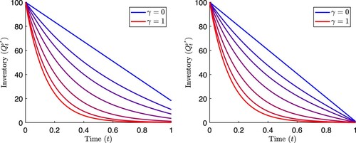n Figure 4 we show the optimal inventory process for several values of the risk-aversion parameter γ. We note that for larger values of γ, the agent uses a trading strategy which liquidates faster towards the beginning of the time interval. This is because the agent's risk is largest when her inventory is largest, and to lower that risk she desires to lower her inventory quickly. This comes at an increased cost due to the temporary price impact. When the agent is risk-neutral (and has a resulting inventory path from (17(17) $Q_t^{{\nu }^{\ast }}=\frac{2k+(2\alpha -b)(T-t)}{2k+(2\alpha -b)T}{q}_0,$(17) )), she trades at a constant rate through time which is determined only by the trade-offs between temporary price impact, permanent price impact, and the liquidation penalty. The optimal strategies of Propositions 3.1 and 3.2 are the result of many simplifying assumptions regarding the dynamics of trading in a market as well as the agent's goals, but they still offer a benchmark to which many other strategies may be compared. In the following sections, we explore work that expands upon the previous results by considering more realistic market dynamics, alternate goals of market participants, or the inclusion of other phenomena.

Figure 4. Optimal inventory process for various values of risk-aversion parameter γ. The curve corresponding to $\gamma =0$ is from Equation (17(17) $Q_t^{{\nu }^{\ast }}=\frac{2k+(2\alpha -b)(T-t)}{2k+(2\alpha -b)T}{q}_0,$(17) ), the remaining curves are from Equation (26(26) $Q_t^{{\nu }^{\ast }}=\frac{{\psi }^{-}{e}^{-\omega (T-t)}+{\psi }^{+}{e}^{\omega (T-t)}}{{\psi }^{-}{e}^{-\omega T}+{\psi }^{+}{e}^{\omega T}}{q}_0.$(26) ). Left panel: $\alpha =0.05$. Right panel: $\alpha =1$. Other parameter values are T = 1, $\sigma =1$, k = 0.01, and b = 0.01.

4. Alternative Dynamics

We begin our further exploration by considering works which make alternative assumptions about the dynamics proposed in Equations (5(5) $\begin{array}{rl}\mathrm{d}{Q}_t^{\nu }& ={\nu }_t\mathrm{d}t,\end{array}$(5) ) to (8(8) $\begin{array}{rl}{\hat{S}}_t^{\nu }& =S_t^{\nu }+g\left({\nu }_t\right),\end{array}$(8) ) in order to model more general or more realistic market settings.

4.1. Stochastic Temporary and Permanent Price Impact

First we revisit one of our assumptions on the nature of price impact, both permanent and temporary. In Equations (6(6) $\begin{array}{rl}\mathrm{d}{S}_t^{\nu }& =f\left({\nu }_t\right)\mathrm{d}t+\mathrm{d}{M}_t,\end{array}$(6) ) and (8(8) $\begin{array}{rl}{\hat{S}}_t^{\nu }& =S_t^{\nu }+g\left({\nu }_t\right),\end{array}$(8) ), the relation between the agent's trading and price dynamics are homogeneous in time – identical actions and different points in time will have identical effects on the asset price. In terms of the graphical representation of the (idealized continuous) LOB, this means that its general shape is always the same, albeit translated horizontally as the midprice changes. In reality, market liquidity varies through time meaning the shape of our graphical representation should also fluctuate. We consider in some detail the work Barger and Lorig (2019) which allows price impact effects to be stochastic, replacing price and wealth dynamics with (29) $\begin{array}{rl}\mathrm{d}{S}_t^{\nu }& =\hat{f}\left(b_t\right){\nu }_t\mathrm{d}t+\sigma \mathrm{d}{W}_t,\mathrm{d}{b}_t={\mu }_b\left(b_t\right)\mathrm{d}t+{\eta }_b\left(b_t\right)\mathrm{d}{B}_t^{\left(1\right)},\end{array}$(29) (30) $\begin{array}{rl}\mathrm{d}{X}_t^{\nu }& =-{\hat{S}}_t^{\nu }{\nu }_t\mathrm{d}t,\end{array}$(30) (31) $\begin{array}{rl}{\hat{S}}_t^{\nu }& =S_t^{\nu }+\hat{g}\left(k_t\right){\nu }_t,\mathrm{d}{k}_t={\mu }_k\left(k_t\right)\mathrm{d}t+{\eta }_k\left(k_t\right)\mathrm{d}{B}_t^{\left(2\right)},\end{array}$(31) where $B^{\left(1\right)}$ and $B^{\left(2\right)}$ are Brownian motions independent of W, but have instantaneous correlation with each other equal to $\rho \in [-1,1]$. Furthermore, the functions $\hat{g}$, ${\mu }_k$, and ${\eta }_k$ should be chosen so that $\hat{g}\left(k_t\right)>0$ for all t (otherwise temporary price impact would work in the agent's favour and she could make unbounded profits). In this model, price impact depends linearly on trading speed (as was assumed in Propositions 3.1 and 3.2), but the magnitude of the effect is driven by the stochastic processes b and k. The graphical LOB representation is therefore given by a flat line which fluctuates through time in the vertical direction. When $\hat{f}\left(b_t\right)$ and $\hat{g}\left(k_t\right)$ decrease, indicating a low impact state, the flat line level of the LOB moves up and there is high liquidity in the market.

The agent's performance criterion is taken as stated in (25(25) $\mathbb{E}[X_T^{\nu }+Q_T^{\nu }(S_T^{\nu }-\alpha Q_T^{\nu })-\frac{\gamma }{2}{\int }_0^T{\sigma }^2(Q_t^{\nu }{)}^2\mathrm{d}t].$(25) ) with a running penalty on inventory, and so as discussed earlier this can be interpreted as the agent being sensitive to the risk associated with midprice changes, but when considering the stochastic nature of price impact she only accounts for the potential benefit and detriment in terms of expected wealth. These changes to the assumed dynamics complicate the HJB analysis which was used to arrive at the conclusions of our previous propositions, so the authors resort to asymptotic approximations of the dynamic value function and optimal trading speed. The authors show that a zeroth order approximation in this setting can be obtained by the same expression as in (24(24) ${\nu }^{\ast }(t,q)=\frac{\left(2h_2\right(t)+b)}{2k}q.$(24) ) by making the substitutions $b\mapsto \hat{f}\left(b\right)$ and $k\mapsto \hat{g}\left(k\right)$. This means the agent acts according to the previously examined optimal strategy, but replaces the price impact parameters with the corresponding value of what is observed at any particular time.

The first order correction to this strategy does not have a simple expression in general. But if the agent is forced to liquidate her position by time T ($\alpha \to \mathrm{\infty }$) and if she does not impose the running inventory penalty ($\gamma =0$), then a first order approximation is given by (32) ${\hat{\nu }}_1^{\ast }(t,q,b,k)={\hat{\nu }}_0^{\ast }(t,q,b,k)-\frac{1}{2}\frac{{\mu }_k\left(k\right){\hat{g}}^{\prime }\left(k\right)}{\hat{g}\left(k\right)}q-\frac{1}{6}\frac{{\mu }_b\left(b\right){\hat{f}}^{\prime }\left(b\right)}{\hat{g}\left(k\right)}(T-t)q,$(32) where the term ${\hat{\nu }}_0^{\ast }$ is understood to be the strategy in (24(24) ${\nu }^{\ast }(t,q)=\frac{\left(2h_2\right(t)+b)}{2k}q.$(24) ) along with the substitutions $b\mapsto \hat{f}\left(b\right)$ and $k\mapsto \hat{g}\left(k\right)$. Note that at any fixed time t with given impact parameters $\hat{f}\left(b_t\right)$ and $\hat{g}\left(k_t\right)$, this first order strategy still liquidates the asset at a speed proportional to the remaining inventory. The two correction terms stem from the two different types of impact and can be interpreted in terms of what the agent expects the impact to be in the future, thereby acting accordingly. If we suppose ${\mu }_k\left(k\right)$ and ${\hat{g}}^{\prime }\left(k\right)$ are both positive, then in the short term, the temporary price impact is expected to increase, so the agent is incentivized to trade faster now to avoid higher transaction costs. Similarly, if we suppose ${\mu }_b\left(b\right)$ and ${\hat{f}}^{\prime }\left(b\right)$ are both positive, then permanent price impact is expected to increase, and the agent should trade faster now so that her remaining pool of shares does not have their value negatively affected. This term depends on the remaining trading time T−t because the effects of permanent price impact as modelled here accumulate over time, and so become insignificant at the end of the trading horizon. Similar arguments hold accordingly if there are changes in sign of ${\mu }_k\left(k\right)$ and ${\hat{g}}^{\prime }\left(k\right)$. Both of these terms are scaled by the instantaneous temporary impact $1/\hat{g}\left(k\right)$ because any expected benefits from trading faster must be weighed against the instantaneous costs of acquiring those benefits.

Numerous other works have also investigated the effects of stochastic liquidity on optimal execution. A similar model is proposed in R. Almgren (2012) where there is no permanent price impact, but the midprice volatility is allowed to be stochastic rather than constant. This work also recognizes that substituting appropriate parameters into a strategy such as (24(24) ${\nu }^{\ast }(t,q)=\frac{\left(2h_2\right(t)+b)}{2k}q.$(24) ) with the observed stochastic counterparts at time t ($k\mapsto k_t$ and $\sigma \mapsto {\sigma }_t$) is a plausible strategy. In general, it is found that the agent trades quickly when price impact is low, volatility is high, or the end of the trading period approaches. Both Cheridito and Sepin (2014) and Ackermann, Kruse, and Urusov (2021) take a fully discrete-time approach to this problem, each considering different aspects of the dynamics to be stochastic and classifying the optimal trading strategies in terms of recursion equations. Other works with elements of stochastic price impact are Ishitani and Kato (2014), Becherer, Bilarev, and Frentrup (2018), Fruth, Schöneborn, and Urusov (2019), Fouque, Jaimungal, and Saporito (2022), and Cartea, Drissi, and Monga (2022), some of which will be discussed in a subsequent section on resilience and transient price impact.

4.2. Stochastic Volatility of Midprice

In the models described in Section 3, the only exogenous source of randomness comes from the midprice innovations which were assumed to have constant volatility. In reality, the volatility will change through time due to a variety of factors in the LOB. There is generally increased activity at the beginning and end of the trading day, both in terms of the number of LOs being placed and cancelled, and in the number of MOs submitted. Each of these events can change the midprice, so we end up with seasonality of volatility in the LOB over the course of the day. Additionally, many events in the LOB are self-exciting, in particular there is a large spike in the intensity of events for a short time after MOs, and so spikes in volatility may also be observed around these times.³ The changing volatility results in different levels of risk for any given inventory level, and accounting for this can help a risk-averse agent improve her performance.

We have already made brief mention of R. Almgren (2012) and Cheridito and Sepin (2014) which consider models with stochastic volatility of the midprice. Here we provide some discussion of Chan and Sircar (2015) which gives approximations to the optimal trading strategy in fast or slow variation volatility regimes, which correspond to the seasonality and spike effects described previously. To this end, we replace the midprice dynamics in Equation (6(6) $\begin{array}{rl}\mathrm{d}{S}_t^{\nu }& =f\left({\nu }_t\right)\mathrm{d}t+\mathrm{d}{M}_t,\end{array}$(6) ) with (33) $\mathrm{d}{S}_t=\sigma \left(Z_t^{ϵ}\right)\mathrm{d}{W}_t,$(33) where σ is a function of the stochastic process $Z^{ϵ}$, which determines the instantaneous volatility of the midprice. Permanent price impact is not considered in Chan and Sircar (2015), but an additional drift term representing an observable signal is included which we have suppressed in our present discussion. We return to the modelling of observable signals in Section 5.1.

When analysing a slow volatility factor, the dynamics of Z are taken as (34) $\mathrm{d}{Z}_t^{ϵ}=ϵ{\mu }_Z\left(Z_t^{ϵ}\right)\mathrm{d}t+\sqrt{ϵ}{\eta }_Z\left(Z_t^{ϵ}\right)\mathrm{d}{B}_t,$(34) where B is a standard Brownian motion independent of W, whereas the fast volatility factor uses dynamics (35) $\mathrm{d}{Z}_t^{ϵ}=\frac{1}{ϵ}{\mu }_Z\left(Z_t^{ϵ}\right)\mathrm{d}t+\frac{1}{\sqrt{ϵ}}{\eta }_Z\left(Z_t^{ϵ}\right)\mathrm{d}{B}_t.$(35) In each case ϵ will act as a parameter of asymptotic expansion which allows for approximations of the optimal strategy when the value of the parameter is small. Chan and Sircar (2015) consider multiscale stochastic volatility with slow and fast factors simultaneously, but we only discuss the resulting effects individually. Additionally, they have assumed an infinitely long trading horizon with a performance criterion of the form (36) $\mathbb{E}[{\int }_0^{\mathrm{\infty }}-\frac{\gamma }{2}{\sigma }^2(Z_t^{ϵ}\left)\right(Q_t^{\nu }{)}^2-k{\nu }_t^2\mathrm{d}t],$(36) which results in a trading strategy that does not explicitly depend on time and brings more focus to the effects of stochastic volatility. Otherwise, the general behaviour of the optimal strategy is largely unchanged from what would arise in a finite horizon. As may be expected after the discussion in Section 4.1, the approximations are largely based on the strategy which maximizes (36(36) $\mathbb{E}[{\int }_0^{\mathrm{\infty }}-\frac{\gamma }{2}{\sigma }^2(Z_t^{ϵ}\left)\right(Q_t^{\nu }{)}^2-k{\nu }_t^2\mathrm{d}t],$(36) ) when volatility is assumed constant. This can be shown to be ${\nu }_0^{\ast }(q;{\sigma }^2)=-\sqrt{\frac{\gamma {\sigma }^2}{2k}}q,$ which is equivalent to (24(24) ${\nu }^{\ast }(t,q)=\frac{\left(2h_2\right(t)+b)}{2k}q.$(24) ) in the limit $T\to \mathrm{\infty }$.

Under slow scale volatility, the approximation of the optimal strategy is found through perturbation analysis of the HJB equation. The resulting strategy in feedback form is ${\hat{\nu }}^{\ast }(q,z)={\nu }_0^{\ast }(q;{\sigma }^2(z\left)\right)=-\sqrt{\frac{\gamma {\sigma }^2\left(z\right)}{2k}}q,$ which we note involves a similar substitution to previously discussed approximations, where parameters are replaced with their currently observed values through time. We also see that this approximation does not include an explicit dependence on the parameter ϵ. The smallest order corrections considered in Chan and Sircar (2015) involves a stochastic drift correlated to the slow scale volatility. In this case the appropriate correction is proportional to $\sqrt{ϵ}$ as well as the correlation between the drift and volatility.

The fast scale volatility is treated with singular perturbation analysis to arrive at an approximate optimal control, with resulting approximation given by (37) ${\hat{\nu }}^{\ast }(q,z)={\nu }_0^{\ast }(q;〈{\sigma }^2〉)-\frac{\gamma q}{2k}{\int }_t^{\mathrm{\infty }}\mathbb{E}\left[{\sigma }^2\right(Z_u^{ϵ})-〈{\sigma }^2〉|Z_t^{ϵ}=z]\mathrm{d}u,$(37) where $〈{\sigma }^2〉$ is the long-term expected variance. This expression has contributions from two terms which represent a zeroth order approximation and first order correction. The zeroth order approximation makes a familiar parameter substitution ${\sigma }^2\mapsto 〈{\sigma }^2〉$, but the first order correction involves future expected deviations of the variance from its long-term expected value. If future variance is expected to be larger than the long-term expected variance, then the agent desires faster liquidation of her shares to avoid the associated inventory risk.

Other work of interest is Colaneri et al. (2020) where the authors assume that innovations in asset price are driven by a regime switching pure jump process of the form (38) $\mathrm{d}{S}_t=S_{t^{-}}\mathrm{d}{R}_t,$(38) where R has compensating random measure $\eta (t,Y_{t^{-}},{\nu }_{t^{-}};\mathrm{d}z)\mathrm{d}t$ with Y a finite state Markov chain. While this is not strictly a stochastic volatility model because it lacks a diffusive term, the price innovations $\mathrm{d}{R}_t$ being driven by a Markov chain means that the price process will share some qualitative features of a stochastic volatility model. The dependence of the compensating measure on the trading strategy ν also captures permanent price impact effects. In this case, the more complicated nature of the model leads to numerical methods for computing the optimal strategy.

4.3. Resilience and Transient Impact

Thus far we have only described two types of price impact effects (permanent and temporary) which are included in the models of many algorithmic trading works. But when discussing the nature of price changes after the occurrence of a transaction, there are other dynamical effects at play. In particular, when multiple LOs are filled in the LOB due to a transaction, the resulting gap in the LOB is not replenished instantaneously as Figure 3 suggests. Instead it takes time for LOs to be submitted in place of those that were filled. The rate at which these orders are replenished is called resilience, and thus Figure 3 suggests a market with infinite resilience.

In Figure 5 we show (from the ask side of the book) how resilience might be interpreted in an idealized continuous LOB. After a transaction takes place (filling sell orders in the book), if no further transactions were to occur then these sell orders may gradually be replenished until a new stable best ask price is established. However, if a subsequent transaction were performed after only a short time, then it would be subjected to higher prices than if it had occurred after a long time. This difference in transaction price which depends on the amount of time between trades is called transient price impact.

Figure 5. Ask side of the LOB showing resilience and transient price impact after a trade. The left panel shows minimal spread (best ask price coincides with reference price). In the middle panel, an MO walks the book and exhibits temporary price impact. Immediately after the MO in the right panel, the orders are filled, a new reference price is established due to permanent impact, and the new best ask price will gradually decay back to the new reference price. A subsequent order submitted immediately will be subjected to higher prices than an order submitted after waiting some time.

We focus on describing Chen, Horst, and Tran (2019) in more detail, as the framework is most similar to what has been presented here so far. A general formulation of transient price impact can be incorporated into the dynamics by introducing an impact function and decay kernel, denoted by a strictly increasing function h and a non-increasing function G, respectively, and defining the inventory, midprice, and cash processes by (39) $\begin{array}{rl}{Q}_t^{\nu }& =Q_0+{\int }_0^t{\nu }_u\mathrm{d}u,\end{array}$(39) (40) $\begin{array}{rl}{S}_t^{\nu }& =S_0+{\int }_0^{t}b{\nu }_u\mathrm{d}u+{\int }_0^{t}h\left({\nu }_u\right)G(|t-u|)\mathrm{d}u+\sigma W_t,\end{array}$(40) (41) $\begin{array}{rl}{X}_t^{\nu }& =X_0-{\int }_0^t{\hat{S}}_u^{\nu }{\nu }_u\mathrm{d}u,\end{array}$(41) (42) $\begin{array}{rl}{\hat{S}}_t^{\nu }& =S_t^{\nu }+k{\nu }_t.\end{array}$(42) Here we have taken the permanent and temporary price impacts to be linear with proportionality constants b and k. The function h determines the magnitude of transient price impact and the decay kernel G controls how quickly the impact of trading decays through time. In Chen, Horst, and Tran (2019) the transient impact is linear with $h\left(\nu \right)=\lambda \nu$ and the decay is exponential with $G(|t-u|)=\exp (-\rho |t-u|)$. Thus, the parameter λ determines the distance from the new reference midprice to the best ask in the right panel of Figure 5, and the distance between the best ask and the new reference midprice decays exponentially. See Gatheral (2010) for some detailed discussion of other impact functions and decay kernels, and consequences of different models with respect to statistical arbitrage opportunities.

The agent is risk-neutral, but with the additional constraint that the inventory process must satisfy $Q_T^{\nu }=0$. Thus, the performance criterion reduces to (43) $H^{\nu }(x_0,q_0,S_0)=\mathbb{E}\left[X_T^{\nu }\right],$(43) and the agent attempts to maximize this over trading speeds $\{{\nu }_t{\}}_{t\in [0,T]}$ which fully liquidate the inventory by time T. Recall that this type of constraint can be applied formally to the strategy given in Proposition 3.1 by taking $\alpha \to \mathrm{\infty }$, and it is to the trading strategies in this limit that we shall compare the optimal strategy with transient impact. Other works mentioned at the end of this section allow for strategies that do not fully liquidate the position by incorporating a liquidation penalty.

Proposition 4.1

The trading strategy which maximizes (43(43) $H^{\nu }(x_0,q_0,S_0)=\mathbb{E}\left[X_T^{\nu }\right],$(43) ) is given by (44) ${\nu }_t^{\ast }=-\frac{\varphi \left(\right({\varphi }^{2}k-\lambda \rho )(\rho \cosh \left(\frac{\varphi T}{2}\right)+\varphi \sinh \left(\frac{\varphi T}{2}\right))+\lambda {\rho }^2\cosh \left(\varphi (t-\frac{T}{2})\right))}{\varphi \rho T\cosh \left(\frac{\varphi T}{2}\right)({\varphi }^{2}k-\lambda \rho )+\sinh \left(\frac{\varphi T}{2}\right)\left(\lambda \rho \right(2\rho -{\varphi }^{2}T)+{\varphi }^{4}kT)}{q}_0,$(44) which results in the inventory process (45) $Q_t^{{\nu }^{\ast }}=q_0-q_0\left(\frac{A+Bt+C\sinh \left(\varphi (t-\frac{T}{2})\right)}{2A+BT}\right),$(45) where (46) $\begin{array}{rl}\varphi & =\sqrt{\rho (\rho +\frac{\lambda }{k})},\end{array}$(46) (47) $\begin{array}{rl}A& =\frac{\lambda }{k}\sinh \left(\frac{\varphi T}{2}\right),\end{array}$(47) (48) $\begin{array}{rl}B& =\varphi \rho \cosh \left(\frac{\varphi T}{2}\right)+{\varphi }^2\sinh \left(\frac{\varphi T}{2}\right),\end{array}$(48) (49) $\begin{array}{rl}C& =\frac{\lambda }{k}.\end{array}$(49)

In Figure 6 we show the optimal trading speed and resulting inventory for various values of the transient impact parameter λ (top row) and decay rate ρ (bottom row). When $\lambda =0$ the optimal rate of trading is constant at $q_0/T$ which is the TWAP strategy in (19(19) $\begin{array}{rl}\underset{\alpha \to \mathrm{\infty }}{lim}{\nu }^{\ast }(t,q)& =-q\end{array}$(19) ). This is expected because $\lambda =0$ corresponds to the same dynamics given in Equations (5(5) $\begin{array}{rl}\mathrm{d}{Q}_t^{\nu }& ={\nu }_t\mathrm{d}t,\end{array}$(5) ) to (8(8) $\begin{array}{rl}{\hat{S}}_t^{\nu }& =S_t^{\nu }+g\left({\nu }_t\right),\end{array}$(8) ). When $\rho =0$ we also obtain the TWAP strategy, which is consistent with intuition because if there is no resilience, the transient price impact becomes a permanent price impact, so the dynamics are equivalent to Equations (5(5) $\begin{array}{rl}\mathrm{d}{Q}_t^{\nu }& ={\nu }_t\mathrm{d}t,\end{array}$(5) ) to (8(8) $\begin{array}{rl}{\hat{S}}_t^{\nu }& =S_t^{\nu }+g\left({\nu }_t\right),\end{array}$(8) ) with the substitution $b\mapsto b+\lambda$. The last case in which the optimal trading speed is constant is in the limit $\rho \to \mathrm{\infty }$ which again corresponds to the dynamics of (5(5) $\begin{array}{rl}\mathrm{d}{Q}_t^{\nu }& ={\nu }_t\mathrm{d}t,\end{array}$(5) ) to (8(8) $\begin{array}{rl}{\hat{S}}_t^{\nu }& =S_t^{\nu }+g\left({\nu }_t\right),\end{array}$(8) ).

Figure 6. Optimal trading speed and inventory process with transient price impact for various values of transient impact parameter λ and decay coefficient ρ. Top row panels: other parameter values are k = 0.01, b = 0.01, $\rho =1$. Bottom row panels: other parameter values are k = 0.01, b = 0.01, $\lambda =0.3$.

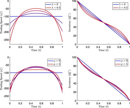
For parameter values which do not give rise to the TWAP strategy, the typical optimal behaviour is to trade at faster speeds closer to the beginning and end of the trading period, and at slower speeds closer to the middle of the trading period (compared to the constant rate of $q_0/T$). The reason for this is because the agent wants to minimize the time when they are trading under significant effect of transient price impact. A single large trade will suffer from temporary price impact, but it is not until subsequent trades are submitted that the effects of transient impact are encountered. By trading quickly early on, there will be more time spent in a state where the exponential resilience has brought the price back towards its unaffected level. Then, when the transient price impact has decayed significantly, the agent can again place large trades to complete the liquidation.

For other descriptions and works which model resilience and transient price impact, see Gatheral (2010), Alfonsi, Fruth, and Schied (2010), Predoiu, Shaikhet, and Shreve (2011), Obizhaeva and Wang (2013), Guo and Zervos (2015), Graewe and Horst (2017), Becherer, Bilarev, and Frentrup (2018), Bank and Voß (2019), Fruth, Schöneborn, and Urusov (2019), Ekren and Muhle-Karbe (2019), Horst and Xia (2019), Forde, Sánchez-Betancourt, and Smith (2021), and Neuman and Voß (2022).

4.4. Non-linear Price Impact

Most of the results in previous sections rely on assuming that price impact functions are linear with respect to the rate of trading, even though the original models proposed in Sections 3.1 and 3.2 have general impact functions. In this section we explore an optimization in which impact functions may be non-linear with respect to the rate of trading, with a focus on R. F. Almgren (2003).

This work begins with a model in discrete time which is based on that of Section 3.1, where the nature of temporary price impact is modified so that Equations (1(1) $Q_{n+1}=Q_n+V_n.$(1) ) to (4(4) $\begin{array}{rl}{\hat{S}}_n& =S_n+g\left(V_n\right).\end{array}$(4) ) become (50) $\begin{array}{rl}{Q}_{n+1}& =Q_n+V_n,\end{array}$(50) (51) $\begin{array}{rl}{S}_{n+1}& =S_n+f\left(V_n\right)+{ϵ}_{n+1},\end{array}$(51) (52) $\begin{array}{rl}{X}_{n+1}& =X_n-{\hat{S}}_n{V}_n,\end{array}$(52) (53) $\begin{array}{rl}{\hat{S}}_n& =S_n+g\left(V_n\right)+h\left(V_n\right){\xi }_{n+1},\end{array}$(53) where $\{\xi {\}}_{n=1}^N$ is a sequence of independent random variables with mean zero, unit variance, and which are also independent from $\{{ϵ}_n{\}}_{n=1}^N$. Thus, the temporary price impact is composed of the usual term, $g\left(V_n\right)$, which depends only on the trade submitted at time n, but also has a stochastic component given by $h\left(V_n\right){\xi }_{n+1}$. This type of stochastic dependence of temporary impact could be the result of several factors, for example the latency between the time that a trade decision is made and the time at which it is matched against passive orders during which the depth of available orders may have changed. See Cartea and Sánchez-Betancourt (2021a) which considers this stochastic delay directly.

The agent attempts to maximize a mean-variance style criterion with respect to her terminal wealth subject to the constraints $Q_N=0$ and that the sequence $\{V_n{\}}_{n=0}^{N-1}$ is deterministic. The agent's terminal wealth is given by (54) $X_N=X_0+S_0{Q}_0+\sum _{n=0}^{N-1}{Q}_{n}f\left(V_n\right)+\sum _{n=0}^{N-1}{Q}_n{ϵ}_{n+1}-\sum _{n=0}^{N-1}{V}_{n}g\left(V_n\right)-\sum _{n=0}^{N-1}{V}_{n}h\left(V_n\right){\xi }_{n+1},$(54) which, under deterministic trading strategies, has expectation and variance (55) $\begin{array}{rl}\mathbb{E}\left[X_N\right]& =X_0+S_0{Q}_0+\sum _{n=0}^{N-1}{Q}_{n}f\left(V_n\right)-\sum _{n=0}^{N-1}{V}_{n}g\left(V_n\right),\end{array}$(55) (56) $\begin{array}{rl}\mathbb{V}\left[X_N\right]& =\sum _{n=0}^{N-1}{\sigma }^2{Q}_n^2+\sum _{n=0}^{N-1}{V}_n^2{h}^2\left(V_n\right),\end{array}$(56) where ${\sigma }^2=\mathbb{E}\left[{ϵ}_n^2\right]$. Before optimizing the trade-off between these two terms, they are both replaced by their continuous-time analogues (57) $\begin{array}{rl}\mathbb{E}\left[X_T\right]& =X_0+S_0{Q}_0+{\int }_0^T\left(Q_{t}f\right({\nu }_t)-{\nu }_{t}g({\nu }_t\left)\right)\mathrm{d}t,\end{array}$(57) (58) $\begin{array}{rl}\mathbb{V}\left[X_T\right]& ={\int }_0^T({\sigma }^2{Q}_t^2+{\nu }_t^2{h}^2({\nu }_t\left)\right)\mathrm{d}t.\end{array}$(58) The objective of the agent is to maximize the mean-variance criterion (59) $H_0^{\nu }=\mathbb{E}\left[X_T\right]-\frac{\gamma }{2}\mathbb{V}\left[X_T\right].$(59) Recognizing that ${\nu }_t=Q_t^{\prime }$ frames this computation into a standard problem of the calculus of variations. After classifying optimality in R. F. Almgren (2003), closed-form expressions for the strategy are found by allowing the horizon T to approach infinity. First, we investigate the effect of non-linear temporary impact with zero stochastic impact such that (60) $f\left(\nu \right)=b\nu ,g\left(\nu \right)=k{\nu }^m,h\left(\nu \right)=0,$(60) with m>0. In this case the optimal inventory path is given by (61) $Q_t^{{\nu }^{\ast }}=\{\begin{array}{ll}{\displaystyle q_0{(1+\frac{1-m}{1+m}\frac{t}{T^{\ast }})}^{-\frac{1+m}{1-m}},}& \text{if}0<m<1,\\ {\displaystyle q_0\exp \{-\frac{t}{T^{\ast }}\},}& \text{if}m=1,\\ {\displaystyle q_0{(1-\frac{m-1}{m+1}\frac{t}{T^{\ast }})}^{\frac{m+1}{m-1}},}& \text{if}m>1\text{ and }t\le \frac{m+1}{m-1}{T}^{\ast },\end{array}$(61) where (62) $T^{\ast }={\left(\frac{2mk{q}_0^{m-1}}{\gamma {\sigma }^2}\right)}^{\frac{1}{m+1}}.$(62) A comparison with (26(26) $Q_t^{{\nu }^{\ast }}=\frac{{\psi }^{-}{e}^{-\omega (T-t)}+{\psi }^{+}{e}^{\omega (T-t)}}{{\psi }^{-}{e}^{-\omega T}+{\psi }^{+}{e}^{\omega T}}{q}_0.$(26) ) in the limit $T\to \mathrm{\infty }$ shows that it coincides with the optimal strategy above when m = 1. 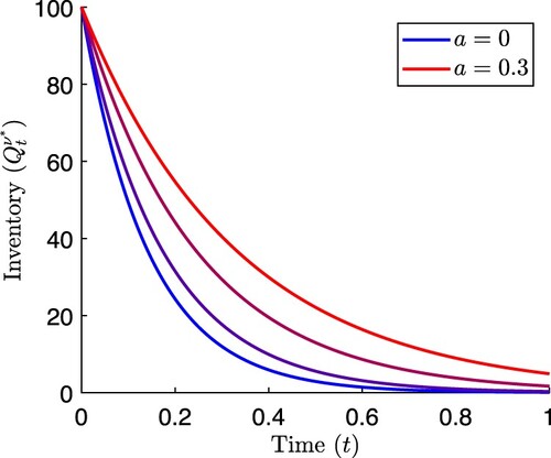This is expected because the price impact functions are the same and the optimal strategy which results from (21(21) $H(t,X_t,Q_t,S_t)=\underset{\nu \in \mathcal{A}}{sup}\mathbb{E}[-\exp \{-\gamma (X_T^{\nu }+Q_T^{\nu }(S_T^{\nu }-\alpha Q_T^{\nu }\left)\right)\}|{\mathcal{F}}_t],$(21) ) is deterministic. The effects of the non-linear impact function g on the optimal strategy are shown in Figure 7. The other case which yields a closed-form expression for the inventory path is (63) $f\left(\nu \right)=b\nu ,g\left(\nu \right)=k\nu ,h\left(\nu \right)=a,$(63) with a>0. The corresponding optimal inventory path is given by (64) $q_0\exp \{-\frac{t}{T^{\ast }}\},$(64) where (65) $T^{\ast }=\sqrt{\frac{2k+\gamma a^2}{\gamma {\sigma }^2}}.$(65) The effect of the stochastic component of price impact can be seen in Figure 8, which is to slow the rate of trading compared to the benchmark of (26(26) $Q_t^{{\nu }^{\ast }}=\frac{{\psi }^{-}{e}^{-\omega (T-t)}+{\psi }^{+}{e}^{\omega (T-t)}}{{\psi }^{-}{e}^{-\omega T}+{\psi }^{+}{e}^{\omega T}}{q}_0.$(26) ). This is because trading quickly magnifies the risks associated with uncertainties in temporary price impact caused by the term $a{V}_n{\xi }_{n+1}$ in (53(53) $\begin{array}{rl}{\hat{S}}_n& =S_n+g\left(V_n\right)+h\left(V_n\right){\xi }_{n+1},\end{array}$(53) ). The agent is willing to accept more risk associated with the uncertainty in future price in order to lower the certain costs and riskiness associated with temporary price impact by trading slower.

Figure 7. Optimal inventory paths from (61(61) $Q_t^{{\nu }^{\ast }}=\{\begin{array}{ll}{\displaystyle q_0{(1+\frac{1-m}{1+m}\frac{t}{T^{\ast }})}^{-\frac{1+m}{1-m}},}& \text{if}0<m<1,\\ {\displaystyle q_0\exp \{-\frac{t}{T^{\ast }}\},}& \text{if}m=1,\\ {\displaystyle q_0{(1-\frac{m-1}{m+1}\frac{t}{T^{\ast }})}^{\frac{m+1}{m-1}},}& \text{if}m>1\text{ and }t\le \frac{m+1}{m-1}{T}^{\ast },\end{array}$(61) ) for various values of parameter m in temporary impact function $g\left(\nu \right)=k{\nu }^m$. Other parameter values are $\sigma =1$, $k=0.01$, b = 0.01, $\gamma =1$.

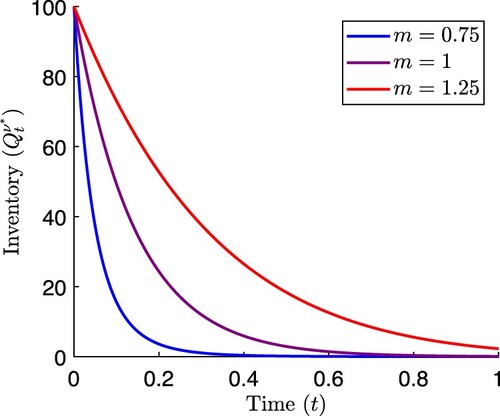
Figure 8. Optimal inventory paths from (64(64) $q_0\exp \{-\frac{t}{T^{\ast }}\},$(64) ) for various values of parameter a in stochastic temporary impact function $h\left(\nu \right)=a$. Other parameter values are $\sigma =1$, $k=0.01$, b = 0.01, $\gamma =1$.

Additional work related to optimal trading with non-linear impact functions can be found in Bouchard, Dang, and Lehalle (2011) and Colaneri et al. (2020). Various discussions are given in Gatheral and Schied (2013) related to the form of impact function and midprice dynamics.

5. Alternative Objectives

In each of the previous sections, the perspective of the optimization problem was that of an agent wishing to liquidate a position subject to various effects related to market dynamics. Within this section, we consider agents who are not necessarily attempting to liquidate some initial holdings, but instead behave according to an alternative objective. Inspection of the optimal trading strategies in previous sections shows that if the agent's inventory begins at zero, then she will do nothing over the course of the trading interval (as her position is already liquidated, any further trading will only be subjected to costs without benefit). Due to the alternative objectives we now consider, this result no longer holds.

5.1. Speculation, Trade Signals, and Statistical Arbitrage

From a modelling perspective, a straightforward method of introducing statistical arbitrage and the ability of an agent to speculate is to assume that the unaffected midprice of the asset is no longer a martingale. In each of the models considered in previous sections, if the agent doesn't trade then the midprice process is a martingale. If instead the unaffected price has non-zero expected change in value over some time interval, then any non-zero inventory position will also be expected to change in value. The essence of a profitable strategy in this situation is to hold inventory positions which take advantage of these non-zero expected price changes, but to do so in an efficient manner so as to not suffer from price impact effects or a future change in the asset's expected drift.

We focus on Cartea and Jaimungal (2016b) which introduces a stochastic drift into the midprice process. The interpretation of the drift in this work is that it arises from the permanent price impact of total order flow of all market participants, but it is statistically equivalent to having a short term price predictor. Let $\mu =\{{\mu }_t{\}}_{0\le t\le T}$ be a stochastic process which satisfies the Markov property, and assume it is adapted to the filtration $\{{\mathcal{F}}_t{\}}_{0\le t\le T}$ we are working with. We specify the dynamics of the relevant processes to be (66) $\begin{array}{rl}\mathrm{d}{Q}_t^{\nu }& ={\nu }_t\mathrm{d}t,\end{array}$(66) (67) $\begin{array}{rl}\mathrm{d}{S}_t^{\nu }& =({\mu }_t+b{\nu }_t)\mathrm{d}t+\sigma \mathrm{d}{W}_t,\end{array}$(67) (68) $\begin{array}{rl}\mathrm{d}{X}_t^{\nu }& =-{\hat{S}}_t^{\nu }{\nu }_t\mathrm{d}t,\end{array}$(68) (69) $\begin{array}{rl}{\hat{S}}_t^{\nu }& =S_t^{\nu }+k{\nu }_t,\end{array}$(69) where b>0 and k>0 are constants. Other than the inclusion of the drift ${\mu }_t$ in (67(67) $\begin{array}{rl}\mathrm{d}{S}_t^{\nu }& =({\mu }_t+b{\nu }_t)\mathrm{d}t+\sigma \mathrm{d}{W}_t,\end{array}$(67) ), these equations are equivalent to (5(5) $\begin{array}{rl}\mathrm{d}{Q}_t^{\nu }& ={\nu }_t\mathrm{d}t,\end{array}$(5) ) to (8(8) $\begin{array}{rl}{\hat{S}}_t^{\nu }& =S_t^{\nu }+g\left({\nu }_t\right),\end{array}$(8) ) (with f and g replaced by linear functions). The value function of our agent will correspond to the performance criterion given in (25(25) $\mathbb{E}[X_T^{\nu }+Q_T^{\nu }(S_T^{\nu }-\alpha Q_T^{\nu })-\frac{\gamma }{2}{\int }_0^T{\sigma }^2(Q_t^{\nu }{)}^2\mathrm{d}t].$(25) ), that is (70) $H(t,X_t,Q_t,S_t,{\mu }_t)=\underset{\nu \in \mathcal{A}}{sup}\mathbb{E}[X_T^{\nu }+Q_T^{\nu }(S_T^{\nu }-\alpha Q_T^{\nu })-\frac{\gamma }{2}{\int }_t^T{\sigma }^2(Q_u^{\nu }{)}^2\mathrm{d}u|{\mathcal{F}}_t],$(70) with $\alpha >0$ and $\gamma >0$ constant. As discussed shortly after (25(25) $\mathbb{E}[X_T^{\nu }+Q_T^{\nu }(S_T^{\nu }-\alpha Q_T^{\nu })-\frac{\gamma }{2}{\int }_0^T{\sigma }^2(Q_t^{\nu }{)}^2\mathrm{d}t].$(25) ), this performance criterion can be interpreted as the agent expressing risk-aversion with respect to the random midprice changes, but risk-neutrality with respect to randomness associated with the stochastic drift process µ.

At this point, no specific dynamics for the process µ have been specified. As long as this stochastic drift term satisfies some technical integrability conditions, the value function and optimal trading strategy can be expressed in terms of expected future drift, as shown in the following Proposition.

Proposition 5.1

The value function in (70(70) $H(t,X_t,Q_t,S_t,{\mu }_t)=\underset{\nu \in \mathcal{A}}{sup}\mathbb{E}[X_T^{\nu }+Q_T^{\nu }(S_T^{\nu }-\alpha Q_T^{\nu })-\frac{\gamma }{2}{\int }_t^T{\sigma }^2(Q_u^{\nu }{)}^2\mathrm{d}u|{\mathcal{F}}_t],$(70) ) is given by (71) $\begin{array}{rl}H(t,x,q,S,\mu )& =x+qS+h_0(t,\mu )+h_1(t,\mu )q+h_2\left(t\right)q^2,\end{array}$(71) (72) $\begin{array}{rl}{h}_2\left(t\right)& =\frac{\text{β}}{2}\frac{{\psi }^{-}{e}^{-\omega (T-t)}-{\psi }^{+}{e}^{\omega (T-t)}}{{\psi }^{-}{e}^{-\omega (T-t)}+{\psi }^{+}{e}^{\omega (T-t)}}-\frac{b}{2},\end{array}$(72) (73) $\begin{array}{rl}{h}_1(t,\mu )& ={\int }_t^T\frac{{\psi }^{-}{e}^{-\omega (T-u)}+{\psi }^{+}{e}^{\omega (T-u)}}{{\psi }^{-}{e}^{-\omega (T-t)}+{\psi }^{+}{e}^{\omega (T-t)}}\mathbb{E}\left[{\mu }_u|{\mathcal{F}}_t\right]\mathrm{d}u,\end{array}$(73) (74) $\begin{array}{rl}{h}_0(t,\mu )& =\frac{1}{4k}{\int }_t^T\mathbb{E}\left[h_1^2\right(t,{\mu }_u\left)|{\mathcal{F}}_t\right]\mathrm{d}u\end{array}$(74) with $\text{β}=\sqrt{2k\gamma {\sigma }^2},\omega =\sqrt{\frac{\gamma {\sigma }^2}{2k}},{\psi }^{\pm }=\text{β}\pm 2\alpha \mp b,$ and the optimal strategy in feedback form is (75) ${\nu }^{\ast }(t,q,\mu )=\frac{h_1(t,\mu )}{2k}+\frac{\left(2h_2\right(t)+b)}{2k}q.$(75)

A comparison of the optimal strategy (75(75) ${\nu }^{\ast }(t,q,\mu )=\frac{h_1(t,\mu )}{2k}+\frac{\left(2h_2\right(t)+b)}{2k}q.$(75) ) to the liquidation strategy without signals given in (24(24) ${\nu }^{\ast }(t,q)=\frac{\left(2h_2\right(t)+b)}{2k}q.$(24) ) shows that the inventory component of the feedback form is identical, but the strategy with signals has an additional component which comes from the agent's forecast of the expected future asset price built into the term $h_1(t,\mu )$. This term could naturally be compared with the more straightforward quantity ${\int }_t^T\mathbb{E}\left[{\mu }_u|{\mathcal{F}}_t\right]\mathrm{d}u$, which represents the expected change in the unaffected midprice from time t to T. While this itself yields a forecast of how much each unit of the agent's inventory is expected to change in value, there are other considerations that the agent must take into account (namely price impact effects, liquidation penalties, and risk) when taking advantage of this signal. This gives rise to the complicated discount factor within the integral which balances the trade-off between taking advantage of the signal while acknowledging that this position will be partially liquidated close to time T and that any inventory holdings have inherent risk of price changes. If we assume $2\alpha >b$,⁴ then inspection of this discount factor shows that it is decreasing from 1 as u ranges from t to T and remains positive. This indicates that the expected price changes in the immediate future as assigned more weight towards the trading strategy compared to expected price changes in the distant future. This arises because the agent would like to enter a position as early as possible to take advantage price changes over as long a time horizon as possible, but also because there is less risk associated with acting on immediate forecasts compared to distant ones.

There are numerous other works in which some form of trade signal or price predictor are incorporated. See for example Chan and Sircar (2015), Cartea, Donnelly, and Jaimungal (2018a), Casgrain and Jaimungal (2019), Lehalle and Neuman (2019), Donnelly and Lorig (2020), Forde, Sánchez-Betancourt, and Smith (2021), Bergault, Drissi, and Guéant (2022), and Neuman and Voß (2022).

5.2. Hedging

The main focus of the previous section was not about optimally liquidating an asset position, but rather attempting to maximize profits that could be extracted from knowledge about expected price changes. Nevertheless, both optimal liquidation and speculative trading have the common theme that they try to minimize costs, or equivalently maximize profits. Here we consider an agent who has an additional objective which is not directly related to cost minimization, although that will still be a consideration which will influence her trading strategy.

In Bank, Soner, and Voß (2017), the authors consider an agent who is tasked with optimally tracking a hedge ratio which arises from attempting to minimize the risk associated with holding another security. Mathematically, they assume that there is a stochastic process $\xi =\{{\xi }_t{\}}_{0\le t\le T}$ which indicates an inventory level which the agent intends to track efficiently. The dynamics of specified processes and the performance criterion used by the agent are given by (76) $\begin{array}{rl}\mathrm{d}{Q}_t^{\nu }& ={\nu }_t\mathrm{d}t,\end{array}$(76) (77) $\begin{array}{rl}\mathrm{d}{X}_t^{\nu }& =-(S_t+k{\nu }_t){\nu }_t\mathrm{d}t,\end{array}$(77) (78) $\begin{array}{rl}{H}^{\nu }(x_0,q_0,S_0)& =\mathbb{E}[X_T^{\nu }+Q_T^{\nu }{S}_T-\frac{1}{2}{\int }_0^T(Q_t^{\nu }-{\xi }_t{)}^2\mathrm{d}t],\end{array}$(78) where the midprice process S is a martingale which is not subject to the effects of permanent price impact. Within the performance criterion, the first two terms reward the agent for trading optimally subject to temporary price impact. The second term gives incentive for the agent to closely track the indicated inventory level ξ.

With an optimization criterion in hand, the authors characterize the optimal trading strategy and value function. For this it is convenient to introduce the notation (79) $\begin{array}{rl}\tau \left(t\right)& =\frac{T-t}{\sqrt{2k}},\end{array}$(79) (80) $\begin{array}{rl}{\hat{\xi }}_t& =\frac{1}{\sqrt{2k}}\mathbb{E}\left[{\int }_t^T\frac{e^{\tau \left(u\right)}+e^{-\tau \left(u\right)}}{e^{\tau \left(t\right)}-e^{-\tau \left(t\right)}}{\xi }_u\mathrm{d}u|{\mathcal{F}}_t\right].\end{array}$(80) Note the similarity between Equations (80(80) $\begin{array}{rl}{\hat{\xi }}_t& =\frac{1}{\sqrt{2k}}\mathbb{E}\left[{\int }_t^T\frac{e^{\tau \left(u\right)}+e^{-\tau \left(u\right)}}{e^{\tau \left(t\right)}-e^{-\tau \left(t\right)}}{\xi }_u\mathrm{d}u|{\mathcal{F}}_t\right].\end{array}$(80) ) and (73(73) $\begin{array}{rl}{h}_1(t,\mu )& ={\int }_t^T\frac{{\psi }^{-}{e}^{-\omega (T-u)}+{\psi }^{+}{e}^{\omega (T-u)}}{{\psi }^{-}{e}^{-\omega (T-t)}+{\psi }^{+}{e}^{\omega (T-t)}}\mathbb{E}\left[{\mu }_u|{\mathcal{F}}_t\right]\mathrm{d}u,\end{array}$(73) ). In Equation (73(73) $\begin{array}{rl}{h}_1(t,\mu )& ={\int }_t^T\frac{{\psi }^{-}{e}^{-\omega (T-u)}+{\psi }^{+}{e}^{\omega (T-u)}}{{\psi }^{-}{e}^{-\omega (T-t)}+{\psi }^{+}{e}^{\omega (T-t)}}\mathbb{E}\left[{\mu }_u|{\mathcal{F}}_t\right]\mathrm{d}u,\end{array}$(73) ), the relevant quantity at any point in time is not the trade signal ${\mu }_t$ itself, but instead the optimal strategy depends on the expected value of the signal at all times in the future, modified according to an integration kernel. A similar theme occurs in (80(80) $\begin{array}{rl}{\hat{\xi }}_t& =\frac{1}{\sqrt{2k}}\mathbb{E}\left[{\int }_t^T\frac{e^{\tau \left(u\right)}+e^{-\tau \left(u\right)}}{e^{\tau \left(t\right)}-e^{-\tau \left(t\right)}}{\xi }_u\mathrm{d}u|{\mathcal{F}}_t\right].\end{array}$(80) ) where the relevant quantity to the optimal efficient hedging strategy is not the intended hedging target ${\xi }_t$, but a weighted average of the expected future value of the target. The precise way that the target hedge ratio enters the optimal trading strategy is summarized by the following proposition.

Proposition 5.2

The value function corresponding to the performance criterion in (78(78) $\begin{array}{rl}{H}^{\nu }(x_0,q_0,S_0)& =\mathbb{E}[X_T^{\nu }+Q_T^{\nu }{S}_T-\frac{1}{2}{\int }_0^T(Q_t^{\nu }-{\xi }_t{)}^2\mathrm{d}t],\end{array}$(78) ) is given by (81) $\begin{array}{rl}H(x_0,q_0,S_0)& =x_0+q_0{S}_0-\sqrt{\frac{k}{2}}\tanh \left(\tau \right(0\left)\right)(q-{\hat{\xi }}_0{)}^2\\ & -\frac{1}{2}\mathbb{E}\left[{\int }_0^T\right(\xi -{\hat{\xi }}_t{)}^2\mathrm{d}t]-\sqrt{\frac{k}{2}}\mathbb{E}[{\int }_0^T\tanh (\tau \left(t\right))d〈\hat{\xi }{〉}_t],\end{array}$(81) and the trading strategy which achieves this performance yields an inventory process that satisfies (82) $\mathrm{d}{Q}_t=\frac{\tanh \left(\tau \right(t\left)\right)}{\sqrt{2k}}({\hat{\xi }}_t-Q_t)\mathrm{d}t,Q_0=q_0.$(82)

In Equation (82(82) $\mathrm{d}{Q}_t=\frac{\tanh \left(\tau \right(t\left)\right)}{\sqrt{2k}}({\hat{\xi }}_t-Q_t)\mathrm{d}t,Q_0=q_0.$(82) ) we see that at any time, the agent will trade such that her inventory moves towards the weighted target ${\hat{\xi }}_t$ with speed being proportional to the current hedging error, with the coefficient being a function depending on the remaining time T−t and the temporary price impact parameter k. This function increases with respect to the remaining time, indicating that the agent puts more effort into tracking the hedge ratio when there is a long amount of time remaining in the trading interval. Indeed, when close to the end of the trading horizon, the performance criterion has relatively small penalty associated with the remaining tracking error, so the agent deems it more efficient to minimize the losses due to trading rather than holding an accurate hedge.

In Bank, Soner, and Voß (2017) the authors also solve this hedge tracking problem when a terminal inventory constraint is imposed of the form $Q_T^{\nu }={\mathrm{\Xi }}_T$, for a given ${\mathrm{\Xi }}_T\in L^2(\mathrm{\Omega },{\mathcal{F}}_T,\mathbb{P})$. Other works related to efficient hedging include R. Almgren and Li (2016), Guéant and Pu (2017), and Ekren and Nadtochiy (2022) in which an agent holds a European option on the traded asset and attempts to maximize the expected utility or mean-variance performance of her terminal wealth. The work Cartea, Donnelly, and Jaimungal (2020) is similar except the agent holds a contingent claim on a non-traded risky quantity which is hedged by a correlated asset, and provide closed form trading strategies which approximate the optimal hedge.

5.3. Targeting VWAP

Each of the previous sections considers an agent that measures her performance using a criterion which is internal. That is, there is no sense of measuring performance relative to other market participants or market state. In this section, we consider an agent who wishes to employ a trading strategy with performance measured by the average execution price of her trades relative to the volume weighted average price (VWAP). The time weighted average price (TWAP) can be captured by any trading strategy which trades at a constant speed over the time interval of interest, and such a strategy has already been seen in Equations (19(19) $\begin{array}{rl}\underset{\alpha \to \mathrm{\infty }}{lim}{\nu }^{\ast }(t,q)& =-q\end{array}$(19) ) and (20(20) $\begin{array}{rl}\underset{\alpha \to \mathrm{\infty }}{lim}{Q}_t^{{\nu }^{\ast }}& =\frac{T-t}{T}{q}_0.\end{array}$(20) ). Unlike TWAP, VWAP depends on the actions of all market participants and measures the average transaction price of all trades over a time period, and the uncertainty in the actions of all other market participants makes it a more difficult quantity to target.

Suppose that all trades over our time period of interest occur at a sequence of times denoted $\tau =\{{\tau }_n{\}}_{n=1}^N$, and that the trade at time ${\tau }_n$ has volume $V_n$ which is executed when the midprice is $S_{{\tau }_n}$.⁵ Then the VWAP for this time period is (83) $\frac{\sum _{n=1}^N{V}_n{S}_{{\tau }_n}}{\sum _{n=1}^N{V}_n}.$(83) Working in continuous time, if we denote total order-flow in the market by $\mu =\{{\mu }_t{\}}_{0\le t\le T}$, then the appropriate expression for VWAP is (84) $\frac{{\int }_0^T{\mu }_t{S}_t\mathrm{d}t}{{\int }_0^T{\mu }_t\mathrm{d}t}.$(84) VWAP is a frequently used benchmark for a trading strategy because it represents the trade performance across the entire market, and additionally is easy to compute. When an agent is trying to optimally liquidate a block of shares with performance measured relative to VWAP, she must time her trades throughout the trading interval so that her average trade price is close to this target. The main difficulty is that VWAP is uncertain because there is randomness in future market order-flow. This difficulty is present in addition to trying to maintaining trade efficiency regarding price impact considerations. One method of attempting to target VWAP is to instead target the percentage of volume (POV) at each point in time. This is the approach taken in Cartea and Jaimungal (2016a) which we now focus on.

Let ${\mu }^{\pm }=\{{\mu }_t^{\pm }{\}}_{0\le t\le T}$ denote the order-flow of buy and sell orders in the market, both assumed to be positive. Then the total order-flow at time t including the agent's trading is given by ${\mu }^{+}+{\mu }^{-}+|{\nu }_t|$. The midprice is assumed to be linearly impacted by all order-flow, and so its dynamics are (85) $\mathrm{d}{S}_t^{\nu }=b({\mu }_t^{+}-{\mu }_t^{-}+{\nu }_t)\mathrm{d}t+\mathrm{d}{M}_t,$(85) where M is a martingale independent of ${\mu }^{\pm }$. Similar to Section 5.1 we assume that ${\mu }^{\pm }$ have the Markov property with respect to our filtration. Instead of directly trying to target VWAP, the agent will attempt to track POV through time. Let $\rho \in (0,1)$ be fixed and define ${\chi }_t^{\nu }=\rho ({\mu }^{+}+{\mu }^{-}+|{\nu }_t|)$, and specify the agent's dynamic value function to be (86) $H(t,X_t,Q_t,S_t,{\mu }_t^{\pm })=\underset{\nu \in \mathcal{A}}{sup}\mathbb{E}[X_T^{\nu }+Q_T^{\nu }(S_T^{\nu }-\alpha Q_T^{\nu })-\phi {\int }_t^T(|{\nu }_u|-{\chi }_u^{\nu }{)}^2\mathrm{d}t|{\mathcal{F}}_t],$(86) where $\phi >0$ is a penalty parameter for deviating from POV. To see why the inclusion of the POV target assists in targeting VWAP, suppose that the agent is only selling, meaning ${\nu }_t\le 0$, and that her trading speed exactly matches the percentage of total order-flow, giving ${\nu }_t=-\rho ({\mu }_t^{+}+{\mu }_t^{-}+|{\nu }_t|)$. Then the agent's trades, marked to the midprice as in (84(84) $\frac{{\int }_0^T{\mu }_t{S}_t\mathrm{d}t}{{\int }_0^T{\mu }_t\mathrm{d}t}.$(84) ), are executed at an average value of (87) $\frac{{\int }_0^T{\nu }_t{S}_t^{\nu }\mathrm{d}t}{{\int }_0^T{\nu }_t\mathrm{d}t}=\frac{{\int }_0^T({\mu }_t^{+}+{\mu }_t^{-}+|{\nu }_t|)S_t^{\nu }\mathrm{d}t}{{\int }_0^T({\mu }_t^{+}+{\mu }_t^{-}+|{\nu }_t|)\mathrm{d}t},$(87) and thus she has exactly targeted VWAP. Unfortunately, by following this strategy she will likely fail to liquidate her initial inventory position, and so inclusion of the penalty term in (86(86) $H(t,X_t,Q_t,S_t,{\mu }_t^{\pm })=\underset{\nu \in \mathcal{A}}{sup}\mathbb{E}[X_T^{\nu }+Q_T^{\nu }(S_T^{\nu }-\alpha Q_T^{\nu })-\phi {\int }_t^T(|{\nu }_u|-{\chi }_u^{\nu }{)}^2\mathrm{d}t|{\mathcal{F}}_t],$(86) ) initiates a trade-off between targeting VWAP and efficiently liquidating her inventory as represented by the other terms in the performance criterion.

For the remainder of this analysis we assume that the agent's optimal trading strategy will consist only of selling, meaning we may replace occurrences of $|{\nu }_t|$ with $-{\nu }_t$, resulting in simplified computations. This assumption will likely be the case when the agent's initial inventory is large and positive and when the need for liquidation outweighs the potential benefits from buying shares of the asset due to price forecasts similar to the treatment in Section 5.1. Under this assumption, the value function and optimal strategy are given by the following Proposition.

Proposition 5.3

The value function in (86(86) $H(t,X_t,Q_t,S_t,{\mu }_t^{\pm })=\underset{\nu \in \mathcal{A}}{sup}\mathbb{E}[X_T^{\nu }+Q_T^{\nu }(S_T^{\nu }-\alpha Q_T^{\nu })-\phi {\int }_t^T(|{\nu }_u|-{\chi }_u^{\nu }{)}^2\mathrm{d}t|{\mathcal{F}}_t],$(86) ) is given by (88) $\begin{array}{rl}H(t,x,Q,S,{\mu }^{\pm })& =h_0(t,{\mu }^{\pm })+h_1(t,{\mu }^{\pm })q+h_2\left(t\right)q^2,\end{array}$(88) (89) $\begin{array}{rl}{h}_2\left(t\right)& =-(\hat{\phi }+k){\left(\right(T-t)+\zeta )}^{-1}-\frac{b}{2}\end{array}$(89) (90) $\begin{array}{rl}{h}_1(t,{\mu }^{\pm })& =b{\int }_t^T\frac{(T-s)+\zeta }{(T-t)+\zeta }\mathbb{E}[{\mu }_s^{+}-{\mu }_s^{-}|{\mathcal{F}}_t]\mathrm{d}s\\ & +\frac{2\hat{\phi }\hat{\rho }}{(T-t)+\zeta }{\int }_t^T\mathbb{E}[{\mu }_s^{+}+{\mu }_s^{-}|{\mathcal{F}}_t]\mathrm{d}s\end{array}$(90) (91) $\begin{array}{rl}{h}_0(t,{\mu }^{\pm })& ={\int }_t^T\mathbb{E}[\frac{\left(h_1\right(s,{\mu }_s^{\pm })-2\hat{\phi }\hat{\rho }({\mu }_s^{+}+{\mu }_s^{-}){)}^2}{4(\hat{\phi }+k)}-\hat{\phi }{\hat{\rho }}^2({\mu }_s^{+}+{\mu }_s^{-}{)}^2|{\mathcal{F}}_t]\end{array}$(91) with $\zeta =\frac{2(\hat{\phi }+k)}{2\alpha -b},\hat{\phi }=\phi (1-\rho {)}^2,\hat{\rho }=\rho /(1-\rho ),$ and the optimal trading strategy in feedback form is (92) ${\nu }^{\ast }(t,q,{\mu }^{\pm })=-{\left(\right(T-t)+\zeta )}^{-1}q+\frac{h_1(t,{\mu }^{\pm })-2\hat{\phi }\hat{\rho }({\mu }^{+}+{\mu }^{-})}{2(\hat{\phi }+k)}.$(92)

In (92(92) ${\nu }^{\ast }(t,q,{\mu }^{\pm })=-{\left(\right(T-t)+\zeta )}^{-1}q+\frac{h_1(t,{\mu }^{\pm })-2\hat{\phi }\hat{\rho }({\mu }^{+}+{\mu }^{-})}{2(\hat{\phi }+k)}.$(92) ) the first term which depends on inventory resembles a strategy that targets TWAP, and the remaining term is an adjustment that attempts to profit from expected future price forecasts (as seen from the term which includes $\mathbb{E}[{\mu }_s^{+}-{\mu }_s^{-}|{\mathcal{F}}_t]$) and the desire to closely target POV (as seen in all terms including ${\mu }^{+}+{\mu }^{-}$). Further intuition about the optimal strategy can be gathered when considering first the limit $\alpha \to \mathrm{\infty }$, then the limit $\phi \to \mathrm{\infty }$. The first of these limits ensures that the agent fully liquidates her position by time T, and the second limit drives her to match POV as closely as possible under the full liquidation constraint. Evaluating these limits gives (93) $\underset{\phi \to \mathrm{\infty }}{lim}\underset{\alpha \to \mathrm{\infty }}{lim}{\nu }^{\ast }(t,q,{\mu }^{\pm })=-\frac{1}{T-t}q-\hat{\rho }\left(\right({\mu }^{+}+{\mu }^{-})-\frac{1}{T-t}{\int }_t^T\mathbb{E}[{\mu }_s^{+}+{\mu }_s^{-}|{\mathcal{F}}_t\left]\mathrm{d}s\right).$(93) The dependence on expected future price has disappeared because of the infinite weight associated with full liquidation and volume tracking. The form of makes it clear that the agent's trading strategy has a component which directly depends on the current total order flow ${\mu }^{+}+{\mu }^{-}$, but the influence is adjusted downward due to the influence of future trades.

In Cartea and Jaimungal (2016a) it is also shown how an agent may target VWAP by tracking percentage of cumulative volume (POCV) rather than POV. Other works which consider an agent attempting to match her trade executions to market VWAP are Konishi (2002) and Frei and Westray (2015). Both derive expressions for strategies which minimize the VWAP targeting error, but rely on future knowledge of the total market volume. A study of guaranteed VWAP contracts is conducted in Guéant and Royer (2014), in which an agent guarantees to provide an execution service at VWAP prices, but then mitigates the risk of having entered this contract. See Białkowski, Darolles, and Fol (2008) and Mitchell, Białkowski, and Tompaidis (2020) for empirical studies of strategies which target VWAP.

5.4. Other Objectives

There are numerous other criteria that an agent could consider for the purposes of evaluating the performance of her trading strategy. Here we briefly mention some lines of research that do not explicitly fall into any of the categories of the previous few sections.

In Neuman et al. (2020) the agent is considered to be a central bank, and she is tasked with maintaining a currency peg or currency target zone, the goal of which is to make sure that a particular foreign exchange rate remains within a specified domain. This is done by trading in the underlying currencies and utilizing the permanent price impact from the trades in such a way as to move the exchange rate to its desired value. This task has significant inventory risk associated with it which the central bank wishes to manage. In Neuman and Schied (2022), a similar currency peg context is considered, but in addition to a central bank maintaining the peg there is a strategic investor attempting to disrupt the bank's objective. This is modelled as a stochastic differential game and a Stackelberg equilibrium is established.

The operation of modern markets is strongly dependent on technology, and the frequency at which events occur mean that latency can have an affect on the performance of an execution strategy. From the time that an agent submits her intention to trade until that signal arrives at the matching engine of the exchange, the state of the limit order book may have changed in such a way that the agent's order cannot be filled. In Cartea and Sánchez-Betancourt (2021b) the agent acknowledges that latency can affect whether her submitted orders are executed as expected, and adjusts her performance criterion to account for the fraction of her trades that are filled. See also Moallemi and Sağlam (2013) for some empirical analysis of the effects of latency on optimal execution strategies.

6. Other Phenomena

Below is a small number of other styles of model which do not explicitly fall into any of the previous categories. Many of the ideas explored in the following sections could be adapted in conjunction with the topics explored already. The referenced material should be consulted for the mathematical details used to approach these phenomena.

6.1. Multiple Agents

Each setting considered so far has incorporated the strategic actions of only one agent. Some of the previous models have incorporated total order flow of the market within the dynamics, but any such model does not arise as a result of an optimization procedure carried out by other agents. In reality, no single agent acts in isolation, and their actions will have an effect on the state of the market, thereby altering the actions of other agents. When modelling several agents simultaneously, we move from a stochastic optimization into a stochastic game setting.

In Schied and Zhang (2019) a competitive game is considered between a finite number of agents where they are restricted to trading at discrete times. Continuous-time counterparts ares studied in Strehle (2017) and Neuman and Voß (2021), and in Voß (2022) a two agent setting is considered in which they must both efficiently track an inventory target.

Finite player stochastic differential games generally result in a set of coupled differential equations which can prove to be intractable. Modeling the problem as a mean-field game, appropriate for a large number of agents, often reduces the complexity of the computations. The optimal liquidation problem in a mean field setting is detailed in Huang, Jaimungal, and Nourian (2019) and Fu et al. (2021). In Casgrain and Jaimungal (2020) and Donnelly and Lorig (2020) a mean-field game is used to consider agents who have different methods of speculation about the future price of the asset.

6.2. Robustness

Each of the optimal trading strategies from previous sections depend on a specification of a dynamic model for the price process and other relevant quantities. But the performance of any trading strategy is subject to risks arising from using a misspecified model, thus it is desirable to account for these risks and attempt to formulate a trading strategy which is robust to model error.

In Schied (2013) the optimality of a trading strategy with respect to the underlying model is studied. In Nyström, Aly, and Zhang (2014), Cartea, Donnelly, and Jaimungal  (2018b), and Horst, Xia, and Zhou (2022), the agent's performance criterion accounts for the possibility that the dynamics evolve according to a different model, and she thereby adjusts her trading strategy to compensate.

6.3. Market Making and Liquidation with Limit Orders

The results which have been outlined in previous sections frame a trading strategy in terms of the speed or volume of trades. Keeping in mind the discussion about the LOB structure, an agent can only guarantee that a particular volume of trades be executed if she employs MOs. Here we give references which study the strategic placement of LOs instead of or in conjunction with MOs.

An agent who simultaneously places buy and sell LOs and attempts to maximize profits is considered in Avellaneda and Stoikov (2008). Further work on optimal market making is considered in Guilbaud and Pham (2013), Guéant, Lehalle, and Fernandez-Tapia (2013), Cartea, Jaimungal, and Ricci (2014), Cartea and Jaimungal (2015b), and Cartea, Donnelly, and Jaimungal (2018a).

The incorporation of LOs on only one side of the LOB for use in optimal liquidation is considered in Guéant, Lehalle, and Fernandez-Tapia (2012), Bayraktar and Ludkovski (2014), Guéant and Lehalle (2015), and Cartea and Jaimungal (2015a).

Acknowledgments

The author would like to thank Fayçal Drissi, Matthew Lorig, and Álvaro Cartea for their comments and suggestions which have improved this manuscript.

Disclosure statement

No potential conflict of interest was reported by the author(s).

Notes

1 Other matching rules such as Pro Rata are also used, but the intricate details of how they differ from FIFO will not be necessary for the types of models considered here.

2 The opposite inequality means the original optimization problem in (12(12) $H(t,X_t,Q_t,S_t)=\underset{\nu \in \mathcal{A}}{sup}\mathbb{E}[X_T^{\nu }+Q_T^{\nu }(S_T^{\nu }-\ell \left(Q_T^{\nu }\right)\left)|{\mathcal{F}}_t\right],$(12) ) may lack concavity, and the agent could make infinite profits through price manipulations.

3 See Cartea, Donnelly, and Jaimungal (2018a) for some empirical investigation of LOB event frequency seasonality and self-excitation.

4 Refer to the discussion after Proposition 3.1.

5 We take all of these volumes to be positive whether they are buys or sells. One could alternatively consider the VWAP of only buy or sell trades depending on whether the agent is buying or selling, but typically all trades are considered in practice. Additionally, VWAP is typically measured with respect to the midprice without taking transaction or price impact effects into account.

References

- Ackermann J., Kruse T., and Urusov M. 2021. “Optimal Trade Execution in an Order Book Model with Stochastic Liquidity Parameters.” SIAM Journal on Financial Mathematics 12 (2): 788–822. doi:10.1137/20M135409X.
- Alfonsi A., Fruth A., and Schied A. 2010. “Optimal Execution Strategies in Limit Order Books with General Shape Functions.” Quantitative Finance 10 (2): 143–157. doi:10.1080/14697680802595700.
- Almgren R. 2012. “Optimal Trading with Stochastic Liquidity and Volatility.” SIAM Journal on Financial Mathematics 3 (1): 163–181. doi:10.1137/090763470.
- Almgren R., and Chriss N. 2001. “Optimal Execution of Portfolio Transactions.” The Journal of Risk 3: 5–39. doi:10.21314/JOR.2001.041.
- Almgren R., and Li T. M. 2016. “Option Hedging with Smooth Market Impact.” Market Microstructure and Liquidity 2 (1): Article ID 1650002. doi:10.1142/S2382626616500027.
- Almgren R., Thum C., Hauptmann E., and Li H. 2005. “Direct Estimation of Equity Market Impact.” Risk 18 (7): 58–62.
- Almgren R. F. 2003. “Optimal Execution with Nonlinear Impact Functions and Trading-Enhanced Risk.” Applied Mathematical Finance 10 (1): 1–18. doi:10.1080/135048602100056.
- Avellaneda M., and Stoikov S. 2008. “High-Frequency Trading in a Limit Order Book.” Quantitative Finance 8 (3): 217–224. doi:10.1080/14697680701381228.
- Bank P., Soner H. M., and Voß M. 2017. “Hedging with Temporary Price Impact.” Mathematics and Financial Economics 11 (2): 215–239. doi:10.1007/s11579-016-0178-4.
- Bank P., and Voß M. 2019. “Optimal Investment with Transient Price Impact.” SIAM Journal on Financial Mathematics 10 (3): 723–768. doi:10.1137/18M1182267.
- Barger W., and Lorig M. 2019. “Optimal Liquidation Under Stochastic Price Impact.” International Journal of Theoretical and Applied Finance 22 (2): Article ID 1850059. doi:10.1142/S0219024918500590.
- Bayraktar E., and Ludkovski M. 2014. “Liquidation in Limit Order Books with Controlled Intensity.” Mathematical Finance 24 (4): 627–650. doi:10.1111/mafi.2014.24.issue-4.
- Becherer D., Bilarev T., and Frentrup P. 2018. “Optimal Liquidation Under Stochastic Liquidity.” Finance and Stochastics 22 (1): 39–68. doi:10.1007/s00780-017-0346-2.
- Bechler K., and Ludkovski M. 2017. “Order Flows and Limit Order Book Resiliency on the Meso-Scale.” Market Microstructure and Liquidity 3 (03n04): Article ID 1850006. doi:10.1142/S2382626618500065.
- Bergault P., Drissi F., and Guéant O. 2022. “Multi-Asset Optimal Execution and Statistical Arbitrage Strategies Under Ornstein–Uhlenbeck Dynamics.” SIAM Journal on Financial Mathematics 13 (1): 353–390. doi:10.1137/21M1407756.
- Bertsimas D., and Lo A. W. 1998. “Optimal Control of Execution Costs.” Journal of Financial Markets 1 (1): 1–50. doi:10.1016/S1386-4181(97)00012-8.
- Biais B., Hillion P., and Spatt C. 1995. “An Empirical Analysis of the Limit Order Book and the Order Flow in the Paris Bourse.” The Journal of Finance 50 (5): 1655–1689. doi:10.1111/j.1540-6261.1995.tb05192.x.
- Białkowski J., Darolles S., and Fol G. Le. 2008. “Improving Vwap Strategies: A Dynamic Volume Approach.” Journal of Banking & Finance 32 (9): 1709–1722. doi:10.1016/j.jbankfin.2007.09.023.
- Björk T. 2009. Arbitrage Theory in Continuous Time. Oxford: Oxford University Press.
- Bouchard B., Dang N.-M., and Lehalle C.-A. 2011. “Optimal Control of Trading Algorithms: A General Impulse Control Approach.” SIAM Journal on Financial Mathematics 2 (1): 404–438. doi:10.1137/090777293.
- Cartea Á., Donnelly R., and Jaimungal S. 2017. “Algorithmic Trading with Model Uncertainty.” SIAM Journal on Financial Mathematics 8 (1): 635–671. doi:10.1137/16M106282X.
- Cartea Á., Donnelly R., and Jaimungal S. 2018. “Enhancing Trading Strategies with Order Book Signals.” Applied Mathematical Finance 25 (1): 1–35. doi:10.1080/1350486X.2018.1434009.
- Cartea Á., Donnelly R., and Jaimungal S. 2018. “Portfolio Liquidation and Ambiguity Aversion.” In High-Performance Computing in Finance, edited by M. Dempster, J. Kanniainen, J. Keane, and E. Vynckier, 77–114. New York: Chapman and Hall/CRC.
- Cartea Á., Donnelly R., and Jaimungal S. 2020. “Hedging Nontradable Risks with Transaction Costs and Price Impact.” Mathematical Finance 30 (3): 833–868. doi:10.1111/mafi.v30.3.
- Cartea Á., Drissi F., and Monga M. 2022. “Decentralised Finance and Automated Market Making: Predictable Loss and Optimal Liquidity Provision.” Available at SSRN 4273989.
- Cartea Á., Gan L., and Jaimungal S. 2019. “Trading Co-Integrated Assets with Price Impact.” Mathematical Finance 29 (2): 542–567. doi:10.1111/mafi.2019.29.issue-2.
- Cartea Á., and Jaimungal S. 2015. “Optimal Execution with Limit and Market Orders.” Quantitative Finance 15 (8): 1279–1291. doi:10.1080/14697688.2015.1032543.
- Cartea Á., and Jaimungal S. 2015. “Risk Metrics and Fine Tuning of High-Frequency Trading Strategies.” Mathematical Finance 25 (3): 576–611. doi:10.1111/mafi.2015.25.issue-3.
- Cartea Á., and Jaimungal S. 2016. “A Closed-Form Execution Strategy to Target Volume Weighted Average Price.” SIAM Journal on Financial Mathematics 7 (1): 760–785. doi:10.1137/16M1058406.
- Cartea Á., and Jaimungal S. 2016. “Incorporating Order-Flow into Optimal Execution.” Mathematics and Financial Economics 10 (3): 339–364. doi:10.1007/s11579-016-0162-z.
- Cartea Á., Jaimungal S., and Penalva J. 2015. Algorithmic and High-Frequency Trading. Cambridge: Cambridge University Press.
- Cartea Á., Jaimungal S., and Ricci J. 2014. “Buy Low, Sell High: A High Frequency Trading Perspective.” SIAM Journal on Financial Mathematics 5 (1): 415–444. doi:10.1137/130911196.
- Cartea A., and Sánchez-Betancourt L. 2021. “Optimal Execution with Stochastic Delay.” Available at SSRN 3812324.
- Cartea Á., and Sánchez-Betancourt L. 2021. “The Shadow Price of Latency: Improving Intraday Fill Ratios in Foreign Exchange Markets.” SIAM Journal on Financial Mathematics 12 (1): 254–294. doi:10.1137/19M1258888.
- Casgrain P., and Jaimungal S. 2019. “Trading Algorithms with Learning in Latent Alpha Models.” Mathematical Finance 29 (3): 735–772. doi:10.1111/mafi.2019.29.issue-3.
- Casgrain P., and Jaimungal S. 2020. “Mean-field Games with Differing Beliefs for Algorithmic Trading.” Mathematical Finance 30 (3): 995–1034. doi:10.1111/mafi.v30.3.
- Chan P., and Sircar R. 2015. “Optimal Trading with Predictable Return and Stochastic Volatility.” Available at SSRN 2623747.
- Chen Y., Horst U., and Tran H. H. 2019. “Portfolio Liquidation Under Transient Price Impact–Theoretical Solution and Implementation with 100 Nasdaq Stocks.” Available at SSRN 3504133.
- Cheridito P., and Sepin T. 2014. “Optimal Trade Execution Under Stochastic Volatility and Liquidity.” Applied Mathematical Finance 21 (4): 342–362. doi:10.1080/1350486X.2014.881005.
- Colaneri K., Eksi Z., Frey R., and Szölgyenyi M. 2020. “Optimal Liquidation Under Partial Information with Price Impact.” Stochastic Processes and Their Applications 130 (4): 1913–1946. doi:10.1016/j.spa.2019.06.004.
- Cont R. 2011. “Statistical Modeling of High-Frequency Financial Data.” IEEE Signal Processing Magazine 28 (5): 16–25. doi:10.1109/MSP.2011.941548.
- Cont R., Kukanov A., and Stoikov S. 2014. “The Price Impact of Order Book Events.” Journal of Financial Econometrics 12 (1): 47–88. doi:10.1093/jjfinec/nbt003.
- Donnelly R., and Lorig M. 2020. “Optimal Trading with Differing Trade Signals.” Applied Mathematical Finance 27 (4): 317–344. doi:10.1080/1350486X.2020.1847672.
- Ekren I., and Muhle-Karbe J. 2019. “Portfolio Choice with Small Temporary and Transient Price Impact.” Mathematical Finance 29 (4): 1066–1115. doi:10.1111/mafi.v29.4.
- Ekren I., and Nadtochiy S. 2022. “Utility-Based Pricing and Hedging of Contingent Claims in Almgren-Chriss Model with Temporary Price Impact.” Mathematical Finance 32 (1): 172–225. doi:10.1111/mafi.v32.1.
- Fleming W. H., and Soner H. M. 2006. Controlled Markov Processes and Viscosity Solutions. Vol. 25. New York: Springer Science & Business Media.
- Forde M., Sánchez-Betancourt L., and Smith B. 2021. “Optimal Trade Execution for Gaussian Signals with Power-Law Resilience.” Quantitative Finance 22 (3): 585–596. doi:10.1080/14697688.2021.1950919.
- Fouque J.-P., Jaimungal S., and Saporito Y. F. 2022. “Optimal Trading with Signals and Stochastic Price Impact.” SIAM Journal on Financial Mathematics 13 (3): 944–968. doi:10.1137/21M1394473.
- Frei C., and Westray N. 2015. “Optimal Execution of a VWAP Order: A Stochastic Control Approach.” Mathematical Finance 25 (3): 612–639. doi:10.1111/mafi.2015.25.issue-3.
- Fruth A., Schöneborn T., and Urusov M. 2019. “Optimal Trade Execution in Order Books with Stochastic Liquidity.” Mathematical Finance 29 (2): 507–541. doi:10.1111/mafi.2019.29.issue-2.
- Fu G., Graewe P., Horst U., and Popier A. 2021. “A Mean Field Game of Optimal Portfolio Liquidation.” Mathematics of Operations Research 46 (4): 1250–1281. doi:10.1287/moor.2020.1094.
- Gatheral J. 2010. “No-Dynamic-Arbitrage and Market Impact.” Quantitative Finance 10 (7): 749–759. doi:10.1080/14697680903373692.
- Gatheral J., and Schied A. 2011. “Optimal Trade Execution Under Geometric Brownian Motion in the Almgren and Chriss Framework.” International Journal of Theoretical and Applied Finance 14 (3): 353–368. doi:10.1142/S0219024911006577.
- Gatheral J., and Schied A. 2013. “Dynamical Models of Market Impact and Algorithms for Order Execution.” In Handbook on Systemic Risk, edited by Fouque, Jean-Pierre, and Joseph A. Langsam, 579–599. Cambridge: Cambridge University Press.
- Graewe P., and Horst U. 2017. “Optimal Trade Execution with Instantaneous Price Impact and Stochastic Resilience.” SIAM Journal on Control and Optimization 55 (6): 3707–3725. doi:10.1137/16M1105463.
- Guéant O. 2016. The Financial Mathematics of Market Liquidity: From Optimal Execution to Market Making. Vol. 33. New York: CRC Press.
- Guéant O., and Lehalle C.-A. 2015. “General Intensity Shapes in Optimal Liquidation.” Mathematical Finance 25 (3): 457–495. doi:10.1111/mafi.2015.25.issue-3.
- Guéant O., Lehalle C.-A., and Fernandez-Tapia J. 2012. “Optimal Portfolio Liquidation with Limit Orders.” SIAM Journal on Financial Mathematics 3 (1): 740–764. doi:10.1137/110850475.
- Guéant O., Lehalle C.-A., and Fernandez-Tapia J. 2013. “Dealing with the Inventory Risk: A Solution to the Market Making Problem.” Mathematics and Financial Economics 7 (4): 477–507. doi:10.1007/s11579-012-0087-0.
- Guéant O., and Pu J. 2017. “Option Pricing and Hedging with Execution Costs and Market Impact.” Mathematical Finance 27 (3): 803–831. doi:10.1111/mafi.2017.27.issue-3.
- Guéant O., and Royer G. 2014. “VWAP Execution and Guaranteed VWAP.” SIAM Journal on Financial Mathematics 5 (1): 445–471. doi:10.1137/130924676.
- Guilbaud F., and Pham H. 2013. “Optimal High-Frequency Trading with Limit and Market Orders.” Quantitative Finance 13 (1): 79–94. doi:10.1080/14697688.2012.708779.
- Guo X., and Zervos M. 2015. “Optimal Execution with Multiplicative Price Impact.” SIAM Journal on Financial Mathematics 6 (1): 281–306. doi:10.1137/120894622.
- Horst U., and Xia X. 2019. “Multi-Dimensional Optimal Trade Execution Under Stochastic Resilience.” Finance and Stochastics 23 (4): 889–923. doi:10.1007/s00780-019-00394-3.
- Horst U., Xia X., and Zhou C. 2022. “Portfolio Liquidation Under Factor Uncertainty.” The Annals of Applied Probability 32 (1): 80–123. doi:10.1214/21-AAP1672.
- Huang X., Jaimungal S., and Nourian M. 2019. “Mean-Field Game Strategies for Optimal Execution.” Applied Mathematical Finance 26 (2): 153–185. doi:10.1080/1350486X.2019.1603183.
- Ishitani K., and Kato T. 2014. “Optimal Execution for Uncertain Market Impact: Derivation and Characterization of a Continuous-Time Value Function.” In 2012 Recent Advances in Financial Engineering: Proceedings of the International Workshop on Finance 2012, edited by A. Takahashi, Y. Muromachi, and T. Shibata, 93–116. Tokyo: World Scientific.
- Konishi H. 2002. “Optimal Slice of a VWAP Trade.” Journal of Financial Markets 5 (2): 197–221. doi:10.1016/S1386-4181(01)00023-4.
- Lehalle C.-A., and Mounjid O. 2017. “Limit Order Strategic Placement with Adverse Selection Risk and the Role of Latency.” Market Microstructure and Liquidity 3 (1): 1750009. doi:10.1142/S2382626617500095.
- Lehalle C.-A., and Neuman E. 2019. “Incorporating Signals into Optimal Trading.” Finance and Stochastics 23 (2): 275–311. doi:10.1007/s00780-019-00382-7.
- Mitchell D., Białkowski J., and Tompaidis S. 2020. “Volume-Weighted Average Price Tracking: A Theoretical and Empirical Study.” IISE Transactions 52 (8): 864–889. doi:10.1080/24725854.2019.1688896.
- Moallemi C. C., and Sağlam M. 2013. “Or Forum–The Cost of Latency in High-Frequency Trading.” Operations Research 61 (5): 1070–1086. doi:10.1287/opre.2013.1165.
- Neuman E., and Schied A. 2022. “Protecting Pegged Currency Markets from Speculative Investors.” Mathematical Finance 32 (1): 405–420. doi:10.1111/mafi.v32.1.
- Neuman E., Schied A., Weng C., and Xue X. 2020. “A Central Bank Strategy for Defending a Currency Peg.” Systems & Control Letters 144: Article ID 104761. doi:10.1016/j.sysconle.2020.104761.
- Neuman E., and Voß M. 2021. Trading with the Crowd. arXiv preprint arXiv:2106.09267.
- Neuman E., and Voß M. 2022. “Optimal Signal-Adaptive Trading with Temporary and Transient Price Impact.” SIAM Journal on Financial Mathematics 13 (2): 551–575. doi:10.1137/20M1375486.
- Nyström K., Aly S. M. Ould, and Zhang C. 2014. “Market Making and Portfolio Liquidation Under Uncertainty.” International Journal of Theoretical and Applied Finance 17 (5): Article ID 1450034. doi:10.1142/S0219024914500344.
- Obizhaeva A. A., and Wang J. 2013. “Optimal Trading Strategy and Supply/Demand Dynamics.” Journal of Financial Markets 16 (1): 1–32. doi:10.1016/j.finmar.2012.09.001.
- Pham H. 2009. Continuous-Time Stochastic Control and Optimization with Financial Applications. Vol. 61. Berlin: Springer Science & Business Media.
- Predoiu S., Shaikhet G., and Shreve S. 2011. “Optimal Execution in a General One-Sided Limit-Order Book.” SIAM Journal on Financial Mathematics 2 (1): 183–212. doi:10.1137/10078534X.
- Ranaldo A. 2004. “Order Aggressiveness in Limit Order Book Markets.” Journal of Financial Markets 7 (1): 53–74. doi:10.1016/S1386-4181(02)00069-1.
- Schied A. 2013. “Robust Strategies for Optimal Order Execution in the Almgren–Chriss Framework.” Applied Mathematical Finance 20 (3): 264–286. doi:10.1080/1350486X.2012.683963.
- Schied A., and Zhang T. 2019. “A Market Impact Game Under Transient Price Impact.” Mathematics of Operations Research 44 (1): 102–121. doi:10.1287/moor.2017.0916.
- Sirignano J. A. 2019. “Deep Learning for Limit Order Books.” Quantitative Finance 19 (4): 549–570. doi:10.1080/14697688.2018.1546053.
- Strehle E. 2017. “Optimal Execution in a Multiplayer Model of Transient Price Impact.” Market Microstructure and Liquidity 3 (03n04): Article ID 1850007. doi:10.1142/S2382626618500077.
- Touzi N., and Tourin A. 2013. Optimal Stochastic Control, Stochastic Target Problems, and Backward SDE. Vol. 29. New York: Springer.
- Voß M. 2022. “A Two-Player Portfolio Tracking Game.” Mathematics and Financial Economics 16 (4): 779–809. doi:10.1007/s11579-022-00324-6.
- Yong J., and Zhou X. Y. 1999. Stochastic Controls: Hamiltonian Systems and HJB Equations. Vol. 43. New York: Springer Science & Business Media.